Neutron–neutron scattering length from the reaction $\gamma d\to\pi^{+}nn$
employing chiral perturbation theory

Abstract

We discuss the possibility to extract the neutron-neutron scattering length $a_{nn}$ from experimental spectra on the reaction $\gamma d\to\pi^{+}nn$. The transition operator is calculated to high accuracy from chiral perturbation theory. We argue that for properly chosen kinematics, the theoretical uncertainty of the method can be as low as $0.1$ fm.

FZJ-IKP-TH-2007-13, HISKP-TH-07/12

1 Introduction

A precise knowledge of the neutron-neutron scattering length $a_{nn}$ is, e.g., important for an understanding of the effects of charge symmetry breaking in nucleon–nucleon forces [1]. The scattering length $a_{nn}$ characterizes scattering at low energies. It is related to the on–shell ${}^{1}S_{0}$ scattering amplitude $f^{\mathrm{on}}$ as

$$f^{\mathrm{on}}(p_{r})=\frac{1}{p_{r}\cot\delta(p_{r})-ip_{r}}=\frac{1}{-a_{nn}^{-1}+\frac{1}{2}\,r_{nn}p_{r}^{2}+{\cal O}(p_{r}^{4})-i\,p_{r}},$$ (1)

where $p_{r}$ is the relative momentum between the two neutrons, $\delta(p_{r})$ the scattering phase shift in the ${}^{1}S_{0}$ partial wave and $r_{nn}$ is the effective range. At low energies the terms of order $p_{r}^{4}$ can be neglected to very high accuracy. Obviously, a direct determination of $a_{nn}$ in a scattering experiment is extremely difficult due to the absence of a free neutron target. For this reason, the value for $a_{nn}$ is to be obtained from analyses of reactions where there are three particles in the final state, e.g. $\pi^{-}d\to\gamma nn$ [2, 3, 4] or $nd\to pnn$ [5, 6, 7]. There is some spread in the results for $a_{nn}$ obtained by the various groups. In particular, two independent analyses of the reaction $nd\to pnn$ give significantly different values for $a_{nn}$, namely $a_{nn}=-16.1\pm 0.4$ fm [6] and $a_{nn}=-18.7\pm 0.6$ fm [7], whereas the latest value obtained from the reaction $\pi^{-}d\to\gamma nn$ is $a_{nn}=-18.5\pm 0.3$ fm [4]. At the same time, for the proton-proton scattering length, which is directly accessible, a very recent analysis reports $a_{pp}=-17.3\pm 0.4$ fm [8] after correcting for electromagnetic effects. This means that even the sign of $\Delta_{a}=a_{pp}-a_{nn}$ is not fixed. It should be mentioned, however, that state of the art calculations for the binding energy difference of tritium and ³He suggest that $\Delta_{a}>0$ [9, 10].

In the present work we discuss the possibility to determine $a_{nn}$ from differential cross sections in the reaction $\gamma d\to\pi^{+}nn$. Specifically, we show that one can extract the value of $a_{nn}$ reliably by fitting the shape of a properly chosen momentum spectrum. In this case the main source of inaccuracies, caused by uncertainties in the single–nucleon photoproduction multipole $E_{0+}$, is largely suppressed. Furthermore there is a suppression of the quasi-free pion production at specific angles. We show that at these angular configurations the extraction of $a_{nn}$ can be done with minimal theoretical uncertainty.

Our investigation is based on the recent work of Ref. [11] in which the transition operator for the reaction $\gamma d\to\pi^{+}nn$ was calculated up to order $\chi^{5/2}$ in chiral perturbation theory (ChPT) with $\chi=m_{\pi}/M_{N}\simeq 1/7$, where $m_{\pi}$ ($M_{N}$) is the pion (nucleon) mass. Half-integer powers of $\chi$ in the expansion arise from the unitarity (two– and three–body) cuts (see also [12]). The results of Ref. [11] for the total cross section are in very good agreement with the experimental data. The only input parameter that entered the calculation was the leading single–nucleon photoproduction multipole $E_{0+}$, which was fixed from a fourth-order one-loop calculation of Bernard et al. [13]. The uncertainty in $E_{0+}$ is the main theoretical error in the calculation presented in Ref. [11]. Besides this transition operator, in the present study we use nucleon–nucleon ($NN$) wave functions constructed likewise in the framework of ChPT, namely those of the NNLO interaction of Ref. [14]. This allows us to estimate the theoretical uncertainty which arises from variations in the wave functions. In fact, as soon as we include consistently all terms up to order $\chi^{5/2}$, we expect the ambiguities due to different wave functions not to be larger than a $\chi^{3}$ correction, for only at this order the leading counter term which absorbs these effects enters. This expectation is indeed quantitatively confirmed in the concrete calculations.

Since we work within chiral perturbation theory we can estimate the effect of higher orders in terms of established expansion parameters together with the standard assumption that additional short ranged operators, that enter at higher orders, behave in accordance with the power counting (the so-called naturalness assumption). This method was also applied in Refs. [15, 16], where the reaction $\pi^{-}d\to\gamma nn$ was investigated as a tool to extract $a_{nn}$. However, to know the effect of higher orders for sure, one has to calculate them. Therefore, to derive a reliable uncertainty estimate for the extraction of $a_{nn}$ from the $\gamma d$ reaction, we use our leading order calculation as baseline result and estimate the theoretical uncertainty from the effects of the higher orders that we calculated completely. Based on this, we find a theoretical uncertainty $\delta a_{nn}\lesssim 0.1\ \mbox{fm}.$ We therefore argue that the reaction $\gamma d\to\pi^{+}nn$ appears to be a good tool for the extraction of $a_{nn}$.

To end this section, we remark that in Ref. [17] a method was proposed to extract scattering lengths from $\gamma d$ induced meson production. However, this approach should not be used here, since the momentum transfer is not sufficiently large to use this method and with our explicit calculation of the transition operator we can reach a significantly higher accuracy.

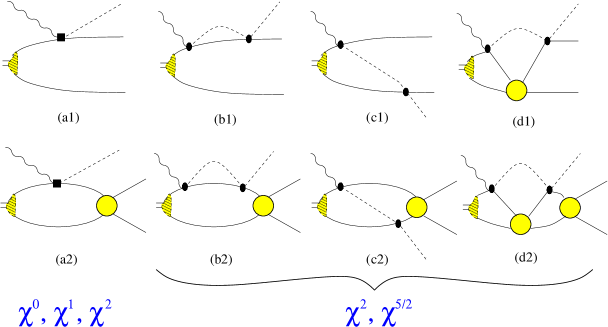
Figure 1: Diagrams for $\gamma d\to\pi^{+}nn$. Shown are one–body terms $\bigl{(}$diagram (a) and (b) $\bigr{)}$, as well as the corresponding rescattering contribution (c)—all without and with final state interaction. Diagrams (d) shows the class of diagrams with intermediate $NN$ interaction. Solid, wavy, and dashed lines denote nucleons, photons and pions, in order. Filled squares and ellipses stand for the various vertices (see Ref. [11] for the details), the hatched area shows the deuteron wave function and the filled circle denotes the $nn$ scattering amplitude. Crossed terms (where the external lines are interchanged) are not shown explicitly.

Figure 2: Kinematical variables for $\gamma d\to\pi^{+}nn$. The relative neutron–neutron momentum is defined as $\vec{p}_{r}=\frac{1}{2}(\vec{p}_{1}-\vec{p}_{2})$.

2 ChPT calculation for $\gamma d\to\pi^{+}nn$

The diagrams that contribute to the reaction $\gamma d\to\pi^{+}nn$ are shown on Fig. 1. The kinematical variables are defined in Fig. 2.

Before going into the details some comments are necessary regarding the relevant scales of the problem. In the near threshold regime of interest here (excess energies of at most 20 MeV above the pion production threshold) the outgoing pion momenta are small compared even to the pion mass. Thus, in addition to the conventional expansion parameters of ChPT $m_{\pi}/\Lambda_{\chi}$ and $q_{\gamma}/\Lambda_{\chi}$, where $\Lambda_{\chi}$ denotes the chiral symmetry breaking scale of order of (and often identified with) the nucleon mass, and $q_{\gamma}$ denotes the photon momentum in the center–of–mass system which is of order of the pion mass, we can also regard $k_{\pi}/m_{\pi}$ as small, where $k_{\pi}$ denotes the momentum of the outgoing pion. In what follows we will perform an expansion in two parameters, namely

$$\chi_{m}=m_{\pi}/M_{N}\ \mbox{and}\ \chi_{Q}=k_{\pi}/m_{\pi}\ .$$

Obviously, the value of the second parameter depends on the excess energy $Q$. The energy regime of interest to us corresponds to excess energies up to 20 MeV. The maximum value of $\chi_{Q}$, $\chi_{Q}^{max}=\sqrt{2Q/m_{\pi}}$, at the highest energy considered is thus about 1/2. Since this is numerically close to $\sqrt{\chi_{m}}$ we use the following assignment for the expansion parameter:

$$\chi\sim\chi_{m}\sim\chi_{Q}^{2}\ .$$ (2)

The tree level $\gamma p\to\pi^{+}n$ vertex, as it appears in diagrams (a1) and (a2) in Fig 1 (the vertex is labeled as filled square), contributes at leading order (order $\chi^{0}$), and orders $\chi^{1}$ and $\chi^{2}$, depending on the one–body operator used. Note that the loop diagrams with $\pi N$ rescattering (see diagrams (b), (c) and (d) in Fig. 1) contribute at order $\chi_{m}^{2}$ as well as at $\chi_{m}^{2}\chi_{Q}$, $\chi_{m}^{5/2}$ and at $\chi_{m}^{1/2}\chi_{Q}^{4}$. The origin of the non–integer power of $\chi$ are the two–body ($\pi N$) and three–body ($\pi NN$) singularities. Thus, all terms up to $\chi^{5/2}$ are explicitly taken into account in our calculation of the transition operator.

As already emphasized, we employ wave functions evaluated in the same framework in order to have a fully consistent calculation. In our work, we use the N²LO wave functions corresponding to the chiral NN forces introduced in Ref. [18] and based on the spectral function regularization (SFR) scheme [19]. At this order, the NN force receives contributions from one-pion exchange, two-pion exchange at the subleading order as well as from all possible short-range contact interactions with up to two derivatives. In addition, the dominant isospin-breaking correction due to the charged-to-neutral pion mass difference in the one-pion exchange potential together with the two leading isospin-breaking S-wave contact interactions were taken into account [18]. The two corresponding low-energy constants were adjusted to reproduce the scattering lengths $a_{nn}$ and $a_{pp}$. The SFR cutoff $\tilde{\Lambda}$ is varied in the range $500\ldots 700$ MeV. It was argued in Ref. [19] that such a choice for $\tilde{\Lambda}$ provides a natural separation of the long- and short-range parts of the nuclear force and allows to improve the convergence of the chiral expansion [19]. The cutoff $\Lambda$ in the Lippmann-Schwinger equation is varied in the range $450\ldots 600$ MeV. For an extensive discussion on the choice of $\Lambda$ and $\tilde{\Lambda}$ the reader is referred to [14, 18].

3 Differential cross sections: relevant features

In this section we outline the features of the differential cross section for unpolarized particles that are important for our considerations. For later convenience let us consider the function $F$ proportional to the square of the matrix element as well as the five–fold differential cross section

$$F(p_{r},\theta_{r},\phi_{r},\theta_{\pi},\phi_{\pi})=C\,p_{r}\ k_{\pi}(p_{r})\overline{|\mathcal{M}(p_{r},\theta_{r},\phi_{r},\theta_{\pi},\phi_{\pi})|^{2}}\propto\frac{d^{5}\sigma(p_{r},\theta_{r},\phi_{r},\theta_{\pi},\phi_{\pi})}{d\Omega_{\vec{p}_{r}}d\Omega_{\vec{k}_{\pi}}dp_{r}^{2}}\ ,$$ (3)

where $\vec{p}_{r}$ ($\vec{k}_{\pi}$) stands for the relative momentum of the two final neutrons (momentum of the final pion) in the center–of–mass frame, $\theta_{r},\ \phi_{r}$ ($\theta_{\pi},\ \phi_{\pi}$) for the corresponding polar and azimuthal angles, respectively, and $\overline{|\mathcal{M}|^{2}}$ for the squared and averaged amplitude. In Eq. (3) $C$ is an irrelevant dimensionful constant. In what follows we will consider only shapes of cross sections and therefore the value of $C$ is not important for our considerations. The value of $k_{\pi}$ at given $p_{r}$ and excess energy $Q$ is fixed by energy conservation:

$$Q=\frac{p_{r}^{2}}{M_{N}}+\frac{k_{\pi}^{2}}{4M_{N}}+\frac{k_{\pi}^{2}}{2m_{\pi}}\,,$$ (4)

hence we write $k_{\pi}(p_{r})$ in Eq. (3).

In the following we choose the momentum $\vec{q}_{\gamma}$ of the initial photon to be along the $z$–axis. Then the cross sections at a certain excess energy $Q$ depend on four variables, namely the magnitude of the relative momentum of the two final neutrons $p_{r}$, the polar angles of the vectors $\vec{p}_{r}$ and $\vec{k}_{\pi}$, and the difference between the azimuthal angles of those two momenta. Unpolarized cross sections are invariant under rotations around the beam axis, which makes the dependence on the missing angle trivial.

Typical differential cross sections $F$ are shown in Fig. 3 as a function of $p_{r}$ at some fixed set of angles $\{\phi_{r},\theta_{\pi},\phi_{\pi}\}$ and $Q=5$ MeV for two different values of $\theta_{r}$. One can see from this figure that for the differential cross section $F$ of Eq. (3) there are two characteristic regions:

1. The region of quasi-free production (QF) at large $p_{r}$, which corresponds to the dominance of those diagrams of Fig. 1 that do not contain the $NN$ interaction in the final or intermediate states. In the Appendix we give explicit expressions for the diagram $a1$ – the most significant diagram of this type. At large $p_{r}$ the pion momentum $k_{\pi}$ is small (see Eq. (4)) and the arguments of the deuteron wave function in Eqs. (A.1) and (A.2) may become small for particular combinations of $\pm\>\vec{p}_{r}$ and $\vec{q}_{\gamma}/2$. This feature gives rise to a peak in the differential cross section at large $p_{r}$.

2. The region with prominence of the strong $nn$ final–state interaction (FSI) at small $p_{r}$ (in fact, we would have the strongest final state interaction at zero relative momentum, however the cross section goes to zero at $p_{r}=0$ due to the phase space, therefore we see a peak shape).

One can see from Fig. 3 that the FSI peak depends on the value of $\theta_{r}$ only marginally, whereas the quasi-free peak shows significant dependence on this angle. In particular, the quasi-free production is largely suppressed at $\theta_{r}=90^{\circ}$ — at this angle the arguments of the wave functions in both terms in the r.h.s. of Eqs. (A.1) and (A.2) are large. It can also be seen from Fig. 3 (right panel) that the effect of higher orders is more important for the quasi-free production amplitude — the influence of higher-order effects on the FSI production is quite small. Another interesting observation is that the contributions of higher orders change the relative height of the two peaks – the FSI peak goes up whereas the QF peak goes down when we proceed from the LO calculation to the order $\chi^{5/2}$. In order to suppress the distortions of the spectrum due to higher orders in the chiral expansion, which is the condition for an extraction of $a_{nn}$ with small theoretical uncertainty, configurations should be chosen where $\theta_{r}=90^{\circ}$.

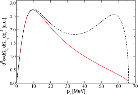
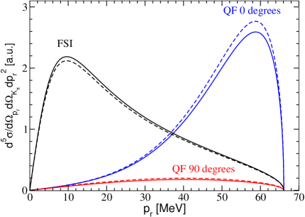
Figure 3: Left panel: Differential cross section. The solid line corresponds to the configuration when the quasi–free peak is suppressed ($\theta_{r}=90^{\circ}$), whereas the dashed line corresponds to one of the configurations when the quasi–free production amplitude is maximal ($\theta_{r}=0^{\circ}$). The values of the remaining angles are $\theta_{\pi}=135^{\circ}$, $\phi_{r}=\phi_{\pi}=0^{\circ}$; they are the same for both curves. Right panel: Differential cross section — relative strength of QF and FSI peaks. Here the dashed curves correspond to the calculation at LO, the solid ones to the calculation at $\chi^{5/2}$. Curves denoted by ”FSI” (”QF”) are obtained by retaining only those diagrams of Fig. 1 that contain (do not contain) the final or the intermediate nucleon–nucleon interaction. The labels ”$0$ degrees” and ”$90$ degrees” denote the corresponding values of $\theta_{r}$ for the ”QF” curves whereas the ”FSI” curves are almost insensitive to this angle. The values or the remaining angles are as on the left panel of this figure. The overall scale is arbitrary in both panels but the relative normalization is the same for all curves.

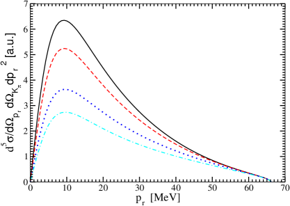
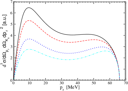
Figure 4: Dependence of the differential cross section on $\theta_{\pi}$. The left panel corresponds to the suppressed quasi–free amplitude ($\theta_{r}=90^{\circ}$), the right panel to the maximal quasi–free amplitude ($\theta_{r}=0^{\circ}$). Solid, dashed, dotted, and dash-dotted lines correspond to $\theta_{\pi}=0^{\circ},\ 45^{\circ},\ 90^{\circ},\ 135^{\circ}$ respectively. The values of the remaining angles are $\phi_{r}=\phi_{\pi}=0^{\circ}$. The overall scale is arbitrary in both panels but the relative normalization is the same for all curves.

We now briefly discuss the dependence of the cross section on the remaining angles $\theta_{\pi},\phi_{\pi}$ (we always may choose $\phi_{r}$ to be zero). The dependence on $\theta_{\pi}$ is illustrated in Fig. 4. One can see from this figure that the dependence on $\theta_{\pi}$ is significant for both the quasi–free as well as the FSI peak. This can be easily understood from the explicit expressions for the matrix elements given in the Appendix keeping in mind that already at $Q=5$ MeV the maximal value of $k_{\pi}$ is about $m_{\pi}/3$ while $q_{\gamma}\approx m_{\pi}$. Thus, the momentum transfer to the nucleon pair, $|\vec{q}_{\gamma}-\vec{k}_{\pi}|$, varies in the range $2m_{\pi}/3$ to $4m_{\pi}/3$ depending on $\theta_{\pi}$. Since the $S$-wave deuteron wave function is large only for very small arguments, the influence of the direction of $\vec{k}_{\pi}$ is significant. In addition, from Fig. 4 it follows that a variation of $\theta_{\pi}$ not only changes the magnitude but also the shape of the cross section, even in the FSI region. This has to be taken into account in the analysis of any experiment.

In contrast to the polar angles, the dependence of $F$ on $\phi_{\pi}$ is negligible for all configurations (there is no dependence at all for $\theta_{r}=0^{\circ}$ and at $\theta_{r}=90^{\circ}$, only the anyway small QF contribution changes by just 5 %).

4 Extraction of $a_{nn}$ and estimate of the theoretical uncertainty

In this section we discuss how to extract the scattering length from future data on $\gamma d\to\pi^{+}nn$ as well as the resulting theoretical uncertainty. Our focus is especially the latter point. As in the previous section we will only discuss results at excess energy $Q=5$ MeV. However, the analysis can be repeated analogously at any excess energy within the range of applicability of the formalism, i.e. $Q\leq 20$ MeV.

We are interested in extracting the value of $a_{nn}$, which, in turn, is a low-energy characteristic of neutron-neutron scattering and manifests itself in the momentum dependence of the cross section at small values of the momentum $p_{r}$. The influence of the value of $a_{nn}$ on the cross section is illustrated in Fig. 5, where the cross sections are shown for three different values of $a_{nn}$, namely $-18,\ -19,\ -20\,$fm. For each value there are two curves, the dashed one corresponds to $\theta_{r}=0^{\circ}$, and the solid one to $\theta_{r}=90^{\circ}$. One can see from Fig. 5 that the influence of different values of $a_{nn}$ is significant in the FSI peak and marginal in the quasi–free peak, as one would have expected.

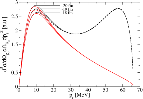
Figure 5: The effect of varying the value of $a_{nn}$ on the differential cross section. The solid and dashed lines correspond to the same angular configurations as in Fig. 3, left panel. The different values of $a_{nn}$ are shown on the figure. The overall scale is arbitrary but the relative normalization is the same for all curves.

In the previous section we have shown (see right panel in Fig. 3) that the relative height of the quasi-free and the FSI peak changes if the effects of higher orders are included in the cross sections. Therefore those angular configurations are to be preferred, where the quasi-free production is suppressed.

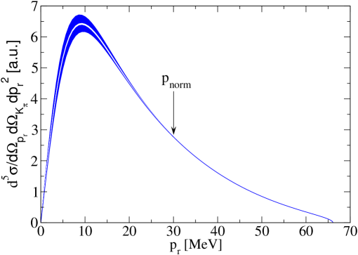
Figure 6: The light (white) band is the error band, and dark (blue) band correspond to $\pm 1\ \mathrm{fm}$ shift in the scattering length from the central value $-18.9\ \mathrm{fm}$.

The central point of this study is to demonstrate that there is a large sensitivity of the momentum spectra to the scattering length and that this scattering length can be extracted with a small and controlled theoretical uncertainty. As outlined in the Introduction, we can estimate this uncertainty reliably, because the effect of the higher orders up to $\chi^{5/2}$ are calculated completely. In order to demonstrate the effect of those higher orders on the shape of the momentum distribution, in Fig. 6 we show as the light band the spread in the results for the calculation from LO to $\chi^{5/2}$. The results also include higher partial waves for the pion as well as the final $nn$ system.

There is some sensitivity to the behavior of the deuteron wave function at short distances. For the reaction $\pi^{-}d\to\gamma nn$ this sensitivity was identified as the largest effect at N³LO in Ref. [15] . Guided by that observation we include in the uncertainty estimate also the spread in the results due to the use of different wave functions. In order to remove the effect of the change in normalization when, e.g., changing the chiral order, all curves are normalized at $p_{\mathrm{norm}}=30$ MeV in Fig. 6. In the same Figure (with the same normalization) we also show the change in the shape that comes from different values of the scattering length: the dark band is generated by a variation of $a_{nn}$ by $\pm 1$ fm around the central value of $-18.9\,$fm. Clearly, the theoretical uncertainty is negligibly small compared to the signal of interest.

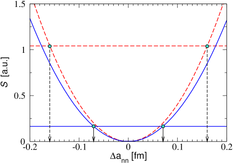
Figure 7: The functions ${\mathcal{S}}(a_{nn}^{(0)},\Phi_{\mathrm{max}})$ and ${\mathcal{S}}(a_{nn}^{(0)}+\Delta a_{nn},\Phi^{(0)})$ are shown by the horizontal and parabolic curves, respectively. The solid curves are obtained by adding the weight factor in Eq. (5) that cuts all momenta above 30 MeV in distinction from the dashed ones. The calculation is performed for the scattering length $a_{nn}^{(0)}=-18.9\ \mathrm{fm}$, $\theta_{r}=90^{\circ}$, and $\theta_{\pi}=0^{\circ}$. The value of $\Delta a_{nn}$ corresponding to the crossing point of the horizontal and parabolic curves determines the theoretical uncertainty of the calculation.

One way to quantify the theoretical uncertainty is through the use of the function ${\mathcal{S}}$, defined as

$${\mathcal{S}}(a_{nn},\Phi)=\int\limits^{p_{\mathrm{max}}}_{0}dp_{r}\>\Bigl{(}F(p_{r}|a_{nn}^{(0)},\Phi^{(0)})-N(a_{nn},\Phi)\ F(p_{r}|a_{nn},\Phi)\Bigr{)}^{2}w(p_{r})\,,$$ (5)

where $p_{\mathrm{max}}=\sqrt{M_{N}Q}$ is the maximum value of $p_{r}$, $F(p_{r}|a_{nn},\Phi)$ is proportional to the five-fold differential cross section as defined in Eq. (3). In the latter we refrained from showing the angular dependence in favor of the parametric dependence of the cross section on the $nn$ scattering length $a_{nn}$ as well as the multi–index $\Phi$, which symbolizes the dependence of the cross section on the chosen chiral order and the wave functions used, as outlined above. The weight function $w(p_{r})$ was introduced to allow us to suppress particular regions of momenta in the analysis — the role of $w(p_{r})$ will be discussed in detail below. For simplicity we may assume that $\mathcal{S}$ is dimensionless; all dimensions can be absorbed into the constant $C$ defined in Eq. (3).

The value $a_{nn}^{(0)}$ denotes the central value of the scattering length ($-18.9$ fm) for which we perform the estimate of the theoretical uncertainty whereas $\Phi^{(0)}$ corresponds to the baseline type of calculation, namely leading order with chiral wave functions as specified in the Appendix. The relative normalization $N(a_{nn},\Phi)$ is fixed by demanding that $\mathcal{S}$ gets minimized for any given pair of parameters $a_{nn},\Phi$ ($\partial{\mathcal{S}}/\partial N=0$). This gives

$$N(a_{nn},\Phi)=\frac{\int\limits^{p_{\mathrm{max}}}_{0}dp_{r}\>F(p_{r}|a_{nn}^{(0)},\Phi^{(0)})F(p_{r}|a_{nn},\Phi)w(p_{r})}{\int\limits^{p_{\mathrm{max}}}_{0}dp_{r}\>F^{2}(p_{r}|a_{nn},\Phi)w(p_{r})}\ .$$ (6)

Obviously $\mathcal{S}$ is the continuum version of the standard $\chi^{2}$ sum, i.e. it characterizes the mean-square deviation from the baseline cross section $F(p_{r}|a_{nn}^{(0)},\Phi^{(0)})$. In this way we determine the theoretical uncertainty in full analogy to the standard method of data analysis.

In order to quantify the theoretical uncertainty we may define $\Phi_{\mathrm{max}}$ as that chiral order and choice of wave function, where ${\mathcal{S}}(a_{nn}^{(0)},\Phi_{\mathrm{max}})$ gets maximal:

$${\mathcal{S}}(a_{nn}^{(0)},\Phi_{\mathrm{max}})=\max_{\Phi}\left\{{\mathcal{S}}(a_{nn}^{(0)},\Phi)\right\}\ .$$ (7)

Therefore ${\mathcal{S}}(a_{nn}^{(0)},\Phi_{\mathrm{max}})$ provides an integral measure of the theoretical uncertainty of the differential cross section. Demanding that the effect of a change in the scattering length by the amount $\Delta a_{nn}$ matches that by the inclusion of higher orders etc., we can identify $\Delta a_{nn}$ as an uncertainty in the scattering length. Expressed in terms of $\mathcal{S}$, we may define $\Delta a_{nn}$ via

$${\mathcal{S}}(a_{nn}^{(0)}+\Delta a_{nn},\Phi^{(0)})={\mathcal{S}}(a_{nn}^{(0)},\Phi_{\mathrm{max}})\ .$$ (8)

This relation is illustrated in Fig. 7. The dashed horizontal line corresponds to ${\mathcal{S}}(a_{nn}^{(0)},\Phi_{\mathrm{max}})$, where we use $w(p_{r})=1$. The dashed parabolic line shows the corresponding ${\mathcal{S}}(a_{nn}^{(0)}+\Delta a_{nn},\Phi^{(0)})$ as a function of $\Delta a_{nn}$. The calculation is performed for $\theta_{r}=90^{\circ}$, and $\theta_{\pi}=0^{\circ}$. The crossing point of the curves corresponds to $\Delta a_{nn}=0.16\ \mathrm{fm}$, which can be identified as the theoretical uncertainty for the extraction of the scattering length.

In the previous section we showed that the signal region is located at momenta lower than $30$ MeV. On the other hand, the theoretical uncertainty of the differential cross section is largest for large values of $p_{r}$ due to the onset of the quasi–free contribution. In view of these two facts it seems reasonable to use such weight functions $w(p_{r})$ that suppress the contribution of large momenta. For instance, we may use $w(p_{r})=\Theta(p^{\mathrm{cut}}-p_{r})$ for the weight function. If we choose, e.g., $p^{\mathrm{cut}}=30$ MeV the theoretical uncertainty of the extraction of the scattering length reduces to $0.07$ fm, as is demonstrated by the solid lines in Fig. 7. This figure nicely illustrates that the parabolic curve that represents the signal changes only very little when a restriction to small values of $p_{r}$ is applied. At the same time this procedure significantly reduces the value of the uncertainty ${\mathcal{S}}(a_{nn}^{(0)},\Phi_{\mathrm{max}})$.

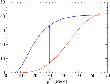
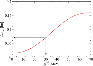
Figure 8: Left panel: Comparison of the $p^{\mathrm{cut}}$ dependence of functions ${\mathcal{S}}(a_{nn}^{(0)},\Phi_{\mathrm{max}}|p^{\mathrm{cut}})$ (dashed curve) and $\alpha(p^{\mathrm{cut}})$ (solid curve). The calculation is performed for the scattering length $a_{nn}^{(0)}=-18.9\ \mathrm{fm}$, $\theta_{r}=90^{\circ}$, and $\theta_{\pi}=0^{\circ}$. Right panel: The corresponding theoretical uncertainty $\Delta a_{nn}$ as a function of $p^{\mathrm{cut}}$.

The observation that the dependence of ${\mathcal{S}}(a_{nn}^{(0)}+\Delta a_{nn},\Phi^{(0)})$ on $\Delta a_{nn}$ is very well approximated by a parabola allows for a more systematic study of the $p^{\mathrm{cut}}$ dependence of the theoretical uncertainty. We therefore define

$$\alpha(p^{\mathrm{cut}})=\frac{{\mathcal{S}}(a_{nn}^{(0)}+\Delta a_{nn},\Phi^{(0)}|p^{\mathrm{cut}})}{(\Delta a_{nn})^{2}}\ ,$$ (9)

where the explicit $p^{\mathrm{cut}}$ dependence is introduced into the function $\mathcal{S}$ through the weight function $w$ as explained above. The dashed and the solid parabola in Fig. 7 can then be written as $\alpha(p^{\mathrm{cut}})\,(\Delta a_{nn})^{2}$, with $\alpha(p_{\mathrm{max}})=41$ fm^-2 and $\alpha(30~{}\mathrm{MeV})=33$ fm^-2. In the left panel of Fig. 8 we show $\alpha(p^{\mathrm{cut}})$ as the solid line. In the same panel the dashed line represents the measure of the theoretical uncertainty given by ${\mathcal{S}}(a_{nn}^{(0)},\Phi_{\mathrm{max}}|p^{\mathrm{cut}})$, multiplied by a factor of 40. This figure makes more quantitative the statement made above: for very small values of $p^{\mathrm{cut}}$ we cut into the signal region and therefore $\alpha$ shows a very rapid variation. However, as soon as $p^{\mathrm{cut}}$ is larger than $30$ MeV it goes to a plateau (in the figure indicated by the arrow). On the other hand, the theoretical uncertainty is monotonously growing once $p^{\mathrm{cut}}$ is larger than $30$ MeV. From this figure we deduce that the ideal value for $p^{\mathrm{cut}}$ is between $25$ and $40$ MeV. This translates into a theoretical uncertainty between $0.05$ and $0.1$ fm, as illustrated in the right panel of the same figure. The value of $\theta_{\pi}$ also has some impact on the theoretical uncertainty, however, in its whole parameter range the estimated uncertainty stays below $0.1$ fm for $p^{\mathrm{cut}}=30$ MeV.

Clearly, also the experimental data, once they exist, should be analyzed using a procedure analogous to the one given above. This means that the scattering length is to be extracted from a $\chi^{2}$ fit of the theoretical curves to the data. In this work we used the calculation at LO as baseline result and the results at higher orders to estimate the theoretical uncertainty. Consequently, we propose to use the momentum spectrum calculated at LO in the fitting procedure of the experiment. The corresponding analytical expressions are given in the Appendix. The only parameter to be adjusted besides the scattering length is the overall normalization. In this fitting procedure only those data points should be included that are below a given $p^{\mathrm{cut}}$, in order to keep the theoretical uncertainty small.

5 Discussion and conclusions

In the previous section it was shown that for the angular configurations that suppress the quasi-free production the inclusion of higher order effects (NLO, N²LO, and $\chi^{5/2}$) as well as the use of different wave functions leads only to a minor change in the momentum dependence of the five-fold differential cross sections.

Based on this observation we propose to use the momentum spectrum calculated at LO for the extraction of the neutron–neutron scattering length from the data. This procedure has the advantage that the corresponding matrix elements can be given in an analytic form (see Appendix) that could be used directly in the Monte Carlo codes for the experiment analysis. In this way the non–trivial dependence of the spectra on $\theta_{\pi}$, discussed above, can be easily controlled. The scattering length can then be extracted by a two parameter fit to the data where, simultaneously to a variation in $a_{nn}$, the normalization constant needs to be adjusted.

Note that the leading order calculation basically agrees to the expression given in Ref. [20] long ago. However, a systematic and reliable study of the theoretical uncertainties of the extraction was possible only within our full calculation up to order $\chi^{5/2}$ in ChPT. In this way we could show that the reaction $\gamma d\to\pi^{+}nn$ is very well suited for a determination of the $nn$ scattering length. The theoretical uncertainty of order $0.1$ fm for the extracted scattering length, estimated in this paper, is of the same order as that claimed for $\pi^{-}d\to\gamma nn$ [16] and $nd\to pnn$ [4, 7].

We discussed in detail the theoretical uncertainty for a fixed excess energy of $Q=5$ MeV only, however, it should be clear that the procedure can be easily repeated for any energy within the range of applicability of our approach ($Q\leq 20$ MeV). For example, we checked that the theoretical uncertainty stays below $0.1$ fm also at $Q=10$ MeV. Note that the number of events in the signal region scales roughly with $\sqrt{Q}$, the phase space available for the pion. It remains to be seen which energy is the best for the corresponding experiment.

We showed that for a proper choice of both kinematics and weight function $w$, the theoretical uncertainty for the extraction of the neutron–neutron scattering length from $\gamma d\to\pi^{+}nn$ can be as low as $0.1$ fm. It should be stressed, however, that this error was evaluated most conservatively – we use our LO calculation as baseline result and estimate the theoretical uncertainty from the effects of the higher orders that we calculated completely. This error can be significantly reduced by further studies. For example, if we include in the uncertainty estimate only the spread in the results due to the use of different wave functions, which is identified as the largest effect at N³LO for the reaction $\pi^{-}d\to\gamma nn$ [15], the theoretical uncertainty of the extracted scattering length reduces by one order of magnitude. This indicates that the theoretical uncertainty is indeed under control. However to put this N³LO estimation on more solid ground a complete calculation should be performed to this order. Most of the operators that are relevant at this order are the same as those of $\pi^{-}d\to\gamma nn$, given explicitly in Ref. [21]. One counter term enters, which can be fixed from other processes [16], e.g., from $nd$ scattering [22], the reaction $NN\to NN\pi$ [23], or from weak decays [16]. Once this is done we may use our calculation to order $\chi^{5/2}$ as baseline result and estimate the theoretical uncertainty from the then available N³LO calculation.

Although we have identified the angles $\theta_{r}=90^{\circ}$ as the preferred kinematics, also other configurations could be studied in order to control the systematics. However, then the spectra calculated at $\chi^{5/2}$ should be used in the analysis.

Appendix A Leading amplitudes

In this appendix we give explicit expressions for the amplitudes that appear at leading order in the calculation for $\gamma d\to\pi^{+}nn$. As outlined in the main text these expressions can be used directly in the analysis of the data, once available. In addition, they should also proof useful for the design of the experiment. Note, as outlined in the text, only near $\theta_{r}=90^{\circ}$ the leading order calculation gives a sufficiently accurate representation of the spectra. At all other angles one should use the complete calculation.

At leading order only diagrams $a1$ and $a2$ of Fig. 1 contribute. Since only the momentum dependence of the amplitudes is relevant for the experimental analysis we drop an overall factor compared to Ref. [11]. The corresponding amplitudes read:

$$M_{a1}^{{s}} = \left(u(\vec{p}_{r}-\vec{k}_{\pi}/2+\vec{q}_{\gamma}/2)+u(-\vec{p}_{r}-\vec{k}_{\pi}/2+\vec{q}_{\gamma}/2)\right)$$ (A.1)

$$M_{a1}^{{t}} = \left(u(\vec{p}_{r}-\vec{k}_{\pi}/2+\vec{q}_{\gamma}/2)-u(-\vec{p}_{r}-\vec{k}_{\pi}/2+\vec{q}_{\gamma}/2)\right)$$ (A.2)

$$M_{a2} = 8\pi\,\frac{f^{\mathrm{on}}(p_{r})}{g(p_{r})}\int\frac{d^{3}\>p}{(2\pi)^{3}}\frac{u(\vec{p}-\vec{k}_{\pi}/2+\vec{q}_{\gamma}/2)\;g(p)}{p^{2}-p_{r}^{2}-i0}\,$$ (A.3)

$$= \frac{f^{\mathrm{on}}(p_{r})}{iq_{\pi\gamma}\>g(p_{r})}\sum_{ij}\frac{C_{i}D_{j}}{p_{r}^{2}+\beta_{j}^{2}}\ \ln\left(\frac{\alpha_{i}-ip_{r}+iq_{\pi\gamma}}{\alpha_{i}-ip_{r}-iq_{\pi\gamma}}\cdot\frac{\alpha_{i}+\beta_{j}-iq_{\pi\gamma}}{\alpha_{i}+\beta_{j}+iq_{\pi\gamma}}\right)$$

where $u(\vec{p})$ denotes the $S$–wave part of the deuteron wave function in momentum space. We checked by explicit calculations that the inclusion of the deuteron $D$-wave changes only the absolute scale of the differential cross sections but not its momentum dependence. Thus, the $D$-wave contribution is not taken into account in the parameterization. The quantity $q_{\pi\gamma}$ is defined as $q_{\pi\gamma}=|\vec{k}_{\pi}-\vec{q}_{\gamma}|/2$. The labels ${s}$ and ${t}$ stand for spin singlet and triplet final two-nucleon states, respectively — we do not write out the corresponding spin structures. We take into account only the ${}^{1}S_{0}$ partial wave in the final state interaction. For a discussion of the effect of $nn$ $P$–waves see Ref. [11].

To derive the expression for $M_{a2}$ we used the fact that the neutron–neutron scattering amplitude can be represented to high accuracy in separable form [11, 24]. The neutron–neutron scattering amplitude, $f(p,k;E)$, can be written in half off–shell kinematics as

$$f(p,k;k^{2}/M_{N})=\frac{2\pi^{2}M_{N}g(p)g(k)}{1-M_{N}\int d^{3}q\frac{g^{2}(q)}{q^{2}-k^{2}-i0}}=f^{\mathrm{on}}(k)\frac{g(p)}{g(k)}\ ,$$ (A.4)

where the corresponding on–shell amplitude $f^{\mathrm{on}}(k)$ can then be expressed in terms of the scattering phase–shifts through

$$f^{\mathrm{on}}(k)=f(k,k;k^{2}/M_{N})=\frac{1}{k\cot\delta(k)-ik}\ .$$

For small momenta one can use the effective range expansion for $k\cot\delta=-1/a_{nn}+r_{nn}k^{2}/2+{\cal O}(k^{4})$, in agreement with Eq. (1). Here $a_{nn}$ is the parameter to be fitted to the data and $r_{nn}=2.76\;$fm. We checked that changing the value of $r_{nn}$ within the bounds allowed ($\pm 0.1$ fm [1]) leads to negligible effects on the extraction of the scattering length. In this way we expressed the matrix element explicitly in terms of the scattering length. We checked that the ratio $g(p)/g(k)$ in Eq. (A.4) does not change when we vary the scattering length within acceptable range bounds.

In order to evaluate the convolution of the deuteron wave function with the $nn$ final state interaction analytically, we needed to employ the following parameterizations for the ${}^{1}S_{0}$ $nn$ form factor $g(p)$ (see Eq. (A.4)) and the S-wave deuteron wave function

$$g(p)=\sum_{i}\frac{D_{i}}{p^{2}+\beta_{i}^{2}};\ \ \ \ u(p)=\sum_{i}\frac{C_{i}}{p^{2}+\alpha_{i}^{2}};$$

where the parameters corresponding to the ChPT calculation at N²LO with cut offs {$\Lambda,\tilde{\Lambda}\}$ = $\{550\$MeV, $\;600\$MeV} (see Ref [18] for details) are listed in Table 1. Note that the coefficients in the parameterization of the wave function have to fulfill the relation $\sum C_{i}=0$ in order to ensure the regularity of the deuteron wave function at the origin in coordinate space [25].

	${}^{1}S_{0}$ form factor		S-wave deuteron w.f.
	$\beta_{i}$ [MeV]	$D_{i}$ [MeV]	$\alpha_{i}$ [MeV]	$C_{i}$ [MeV1/2]
1	164.53278	31.101228	45.334919	43.543212
2	246.85751	-1310.3056	242.66091	-35.643003
3	329.18224	9455.9603	439.98691	419.25214
4	411.50697	-9666.0268	637.31291	-1833.4708
5	493.83170	-55571.615	834.63891	-3710.8173
6	576.15643	64600.071	1031.9649	24903.150
7	658.48116	149128.85	1229.2909	-31673.576
8	740.80589	-84844.967	1426.6169	26476.636
9	823.13062	-295594.17	1623.9429	-118733.48
10	905.45536	-30332.710	1821.2689	259759.15
11	987.78009	560829.89	2018.5949	-223816.07
12	1070.1048	-307006.25	2215.9209	$-\sum_{i=1}^{11}C_{i}$

Table 1: Parameters of the ${}^{1}S_{0}$ form factor and the S-wave deuteron wave function for the separable representation of the N²LO chiral $NN$ potential.

The squared and averaged amplitude to be used in the expression for the differential cross section, defined in Eq. (3) is

$$\overline{|\mathcal{M}(p_{r},\theta_{r},\phi_{r},\theta_{\pi},\phi_{\pi})_{\mathrm{{fit}}}|^{2}}=\left|M_{a1}^{{s}}+M_{a2}\right|^{2}+2\left|M_{a1}^{{t}}\right|^{2}\ .$$ (A.5)

In a fit to data two parameters are to be adjusted, namely the overall normalization $C$ of Eq. (3) and the object of desire, $a_{nn}$.

References

- [1] G. Miller, B. Nefkens and I. Šlaus. Phys. Rep. 194, 1 (1990).
- [2] B. Gabioud et al., Nucl. Phys. A 420, 496 (1984).
- [3] O. Schori et al., Phys. Rev. C 35, 2252 (1987).
- [4] C. R. Howell et al., Phys. Lett. B 444, 252 (1998).
- [5] D. E. Gonzáles Trotter et al., Phys. Rev. Lett. 83, 3788 (1999).
- [6] V. Huhn et al., Phys. Rev. Lett. 85, 1190 (2000); Phys. Rev. C 63, 014003 (2000).
- [7] D. E. Gonzáles Trotter et al., Phys. Rev. C 73, 034001 (2006).
- [8] R. B. Wiringa, V. G. J. Stoks and R. Schiavilla, Phys. Rev. C 51, 38 (1995) [arXiv: nucl-th/9408016].
- [9] R. Machleidt and H. Müther, Phys. Rev. C 63, 034005 (2001) [arXiv:nucl-th/0011057].
- [10] A. Nogga et al., Phys. Rev. C 67, 034004 (2003) [arXiv:nucl-th/0202037].
- [11] V. Lensky, V. Baru, J. Haidenbauer, C. Hanhart, A. Kudryavtsev and U.-G. Meißner, Eur. Phys. J. A 26, 107 (2005) [arXiv: nucl-th/0505039].
- [12] V. Baru, C. Hanhart, A. E. Kudryavtsev and U.-G. Meißner, Phys. Lett. B 589, 118 (2004) [arXiv: nucl-th/0402027].
- [13] V. Bernard, N. Kaiser and U.-G. Meißner, Phys. Lett. B 383, 116 (1996) [arXiv:hep-ph/9603278].
- [14] E. Epelbaum, Prog. Part. Nucl. Phys. 57, 654 (2006) [arXiv: nucl-th/0505032].
- [15] A. Gårdestig and D. R. Phillips, Phys. Rev. C 73, 014002 (2006) [arXiv: nucl-th/0501049].
- [16] A. Gårdestig and D. R. Phillips, Phys. Rev. Lett. 96 (2006) 232301 [arXiv:nucl-th/0603045].
- [17] A. Gasparyan, J. Haidenbauer, C. Hanhart and K. Miyagawa, arXiv:nucl-th/0701090; Eur. Phys. J. A in print.
- [18] E. Epelbaum, W. Glöckle and U.-G. Meißner, Nucl. Phys. A 747, 362 (2005) [arXiv: nucl-th/0405048]
- [19] E. Epelbaum, W. Glöckle and U.-G. Meißner, Eur. Phys. J. A 19, 125 (2004) 125 [arXiv:nucl-th/0304037].
- [20] J. M. Laget, Phys. Rep. 69 (1981) 1.
- [21] A. Gårdestig, Phys. Rev. C 74, 017001 (2006) [arXiv:nucl-th/0604035].
- [22] E. Epelbaum, A. Nogga, W. Glöckle, H. Kamada, U.-G. Meißner and H. Witala, Phys. Rev. C 66, 064001 (2002) [arXiv:nucl-th/0208023].
- [23] C. Hanhart, U. van Kolck and G. A. Miller, Phys. Rev. Lett. 85 (2000) 2905 [arXiv:nucl-th/0004033].
- [24] J. Haidenbauer and W. Plessas, Phys. Rev. C 30, 1822 (1984).
- [25] M. Lacombe, B. Loiseau, R. Vinh Mau, J. Cote, P. Pires and R. de Tourreil, Phys. Lett. B 101, 139 (1981).