Correlated modulation between the redshifted Fe K$\alpha$ line
and the continuum emission in NGC 3783

Abstract

Aims. It has been suggested that X-ray observations of rapidly variable Seyfert galaxies may hold the key to probe the gas orbital motions in the innermost regions of accretion discs around black holes and, thus, trace flow patterns under the effect of the hole strong gravitational field.

Methods. We explore this possibility by re-analyzing the multiple XMM-Newton observations of the Seyfert 1 galaxy NGC 3783. A detailed time-resolved spectral analysis is performed down to the shortest possible time-scales (few ks) using “excess maps” and cross-correlating light curves in different energy bands.

Results. In addition to a constant core of the Fe K$\alpha$ line, we detected a variable and redshifted Fe K$\alpha$ emission feature between 5.3–6.1 keV. The line exhibits a modulation on a time-scale of $\sim$27 ks that is similar to and in phase with a modulation of the 0.3–10 keV source continuum. The two components show a good correlation.

Conclusions. The time-scale of the correlated variability of the redshifted Fe line and continuum agrees with the local dynamical time-scale of the accretion disc at $\sim$10 $\mathrm{r_{g}}$ around a black hole with the optical reverberation mass $\sim$10${}^{7}\mathrm{M_{\odot}}$. Given the shape of the redshifted line emission and the overall X-ray variability pattern, the line is likely to arise from the relativistic region near the black hole, although the source of the few cycles of coherent variation remains unclear.

1 Introduction

The fluorescent iron K (Fe K$\alpha$) emission line is considered to be a useful probe of the accretion flow around the central black hole of an active galaxy. In particular, due to the high orbital velocity and strong gravitational field in the innermost regions of an accretion disc, its profile shall be deformed by the concurrence of Doppler and relativistic shifts. The resulting line is therefore broadened, with a red-wing extending towards lower energies (e.g. Fabian et al. fabian (2000); Reynolds & Nowak reynolds (2003)). Detailed modelling of time-averaged spectra have been used to obtain important estimates of the disc ionization state, its covering factor and, at least for the brightest and best cases, its emissivity law, inner radius and BH spin (Brenneman & Reynolds brenneman (2006); Miniutti et al. miniutti2006 (2006); Guainazzi et al. guainazzi (2006); Nandra et al. nandra2006 (2006)). It is also well established that time-resolved spectral analysis is a fundamental tool if we want to understand not only the geometry and kinematics of the inner accretion flow but also its dynamics. Early attempts (i.e. Iwasawa et al. iwasawa1996 (1996); Vaughan & Edelson vaughan (2001); Ponti et al. ponti (2004); Miniutti et al. miniutti2004 (2004)) have clearly shown that the redshifted component of the Fe K$\alpha$ line is indeed variable and that complex geometrical and relativistic effects should be taken into account (Miniutti et al. miniutti2004 (2004)).
More recently, results of iron line variability have been reported (Iwasawa, Miniutti & Fabian iwasawa2004 (2004); Turner et al. turner (2006); Miller et al. miller2006 (2006)). These are consistent with theoretical studies on the dynamical behaviour of the iron emission arising from localized hot spots on the surface of an accretion disc (e.g. Dovčiak et al. dovciak (2004)). Iwasawa, Miniutti & Fabian (iwasawa2004 (2004)), for example, measured a $\sim$25 ks modulation in the redshifted Fe K$\alpha$ line flux in NGC 3516, which suggests that the emitting region is very close to the central black hole. However, these are likely to be transient phenomena, since such spots are not expected to survive more than a few orbital revolutions. For this reason, it is inherently difficult to establish the observational robustness of these type of models, if not by accumulating further observational data.

Figure 1: The X-ray light curves of NGC 3783 in the 0.3–10 keV band. Left panel: light curve of the 2000 observation. Right panel: light curves of the 2001a and 2001b observations.

Here we present results on the iron line variability in the bright Seyfert galaxy NGC 3783 (z$\simeq$0.01) based on XMM-Newton data. This object has been taken as an example in which multiple warm absorbers can mimic the broad iron line feature (Reeves et al. reeves (2004)), contrary to the initial claim of the presence of a broad iron line emission using ASCA data (Nandra et al. nandra1997 (1997)). However, the recent study by De Marco et al. (demarco (2006)) found evidence for a transient excess feature in the 5–6 keV energy band, interpreted as a redshifted component of the Fe K line. This result is also supported by a variability study by O’Neill & Nandra (oneill (2006)), who examined rms variability spectra of a sample of bright active galaxies observed with XMM-Newton. Given the above considerations, we re-examined all the XMM-Newton observations of NGC 3783 to perform a comprehensive study of the iron line temporal evolution, on the shortest possible time-scale.

2 XMM-Newton observations

XMM-Newton observed NGC 3783 on 2000 December 28–29 and on 2001 December 17–21. The first observation (ID 0112210101) has a duration of $\sim$40 ks while the second (ID 0112210201 and ID 0112210501, hereafter observation 2001a and 2001b respectively) lasts over two complete orbits for a total duration of $\sim$270 ks. Only the EPIC pn data are used in the following analysis because of the high sensitivity in the Fe K band. The EPIC pn camera was operated in the “Small Window” mode with the Medium filter both during the 2000 and the 2001 observations. The live time fraction is thus 0.7. The data were reduced using the XMM-SAS v. 6.5.0 software while the analysis was carried on using the lheasoft v. 5.0 package. High background time intervals were excluded from the analysis. The useful exposure time intervals are listed in Tab. 1, together with the mean 0.3–10 keV count rate for each observation. Only single and double events were selected. Source photons were collected from a circular region of 56 arcsec radius, while the background data were extracted from rectangular, nearly source-free regions on the detector. The background is assumed to be constant throughout the useful exposure. The 0.3–10 keV light curves are shown in Fig. 1 for each observation.

3 Data analysis

3.1 Spectral features of interest and selection of the energy resolution

The time-averaged spectrum was analyzed using the XSPEC v. 11.2 software package. For simplicity, we limited the analysis to the 4–9 keV band. In this energy band, we checked that the complex and highly ionized warm absorber (with log$\xi$ and $N_{\rm H}$ up to $\sim$2.9 erg cm s^-1 and 5$\times$10²² cm^-2, Reeves et al. reeves (2004)) shall not affect our conclusions below. The residuals against a simple power-law plus cold absorption continuum model for the 2001b observation, the longest continuous dataset available, are shown in Fig. 2. In this fit we excluded the Fe K energy band (i.e. 5–7 keV) and the best fit parameters are $(2.5\pm 0.6)\times 10^{22}$ cm^-2 and $1.81\pm 0.04$, for the absorber column density and power-law slope respectively.

Table 1: Date, duration, useful exposure and mean EPIC pn 0.3–10 keV count rate for each XMM-Newton observation of NGC 3783.

Obs. ID	Date	Duration	Exposure	$\langle\mathrm{CR}\rangle$
		(ks)	(ks)	(c/s)
0112210101	2000 Dec 28–29	40.412	35	8.5
0112210201	2001 Dec 17–19	137.818	115	6.5
0112210501	2001 Dec 19–21	137.815	120	8.5

Figure 2: The 4–9 keV residuals against a simple power-law plus cold absorption continuum model for the spectrum of NGC 3783 during the 2001b observation. The data are obtained from EPIC pn.

Identified are four excess emission features: the main Fe K$\alpha$ core at $\sim$6.4 keV, a wing to the line core at around 6 keV, a peak at $\sim$7 keV (possibly Fe K$\beta$) and a narrow peak at $\sim$5.4 keV. Moreover we identified two absorption features at $\sim$6.7 keV and $\sim$7.6 keV. When fitted with Gaussian emission and absorption lines, all these features are significant at more than $\sim$99% confidence level. Similar results were also obtained by a detailed analysis with more complex models (Reeves et al. reeves (2004)). We will focus here on the analysis of the features variability properties. The application of the excess map technique to the identified absorption features did not give significant results, thus, in the following, we will focus on the analysis of emission features variability only. The 2001a observation has been divided into two parts because of the gap in the data between t$\sim$5$\times$10⁴ s and t$\sim$6$\times$10⁴ s. Since all the selected spectral features are comparable to the CCD spectral resolution, we chose 100 eV for the energy resolution of the excess maps.

3.2 Selection of the time resolution

In choosing the time resolution for the excess maps we looked for the best trade-off between getting a sufficiently short time-scale, in order to oversample variability, and keeping enough counts in each energy resolution bin. We first considered the 2001b observation, having the longest and continuous exposure. Spectra were extracted during different time intervals (1 ks, 2.5 ks and 5 ks) around the local minimum flux state at t$\sim$215 ks. The required condition is that each 100 eV energy bin in the 4–9 keV band has to contain at least 50 counts. At the time resolution of 2.5 ks we got $\sim$90 counts per energy bin at the energies of the “red” feature (5.3–5.4 keV), and $\sim$80 counts per energy bin in the “wing” feature energy band (5.8–6.1 keV). Moreover, for a 10⁷ M_⊙ black hole we expect the Keplerian orbital period to be $\sim$10⁴ s at a radius of 10 $\mathrm{r_{g}}$. Thus, selecting 2.5 ks as the excess maps time resolution, enables us to completely oversample this typical time-scale. This choice of time resolution, optimized for the 2001b observation, was extended to the 2000 and 2001a data.

Table 2: Spectral features of interest in the 4–9 keV band with the selected band-passes and mean intensity.

Feature	Energy band	$\langle I\rangle$
	(keV)	($10^{-5}\,\mathrm{ph\,s^{-1}cm^{-2}}$)
red	5.3–5.4	0.6
wing	5.8–6.1	2
core (K$\alpha$)	6.2–6.5	5.3
K$\beta$	6.8–7.1	1.2
Red+Wing	5.3–6.1	3.2

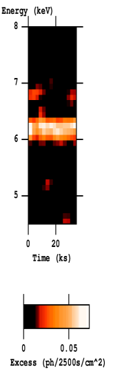
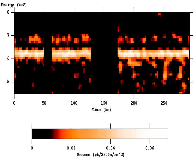
Figure 3: The excess emission maps of the 4–9 keV band in the time-energy plane at 2.5 ks time resolution. The images have been smoothed. Since the 6.4 keV line core is very strong and stable, the color map is adjusted to saturate the line core and allow lower surface brightness features to be visible. Left panel: excess emission map from the 2000 observation. Right panel: excess emission map from the 2001a and 2001b observations.

4 Excess emission maps

Energy spectra for a duration of the chosen exposure time (2.5 ks) are extracted in time sequence. 14 spectra are obtained from the 2000 observation, 46 and 48 spectra are obtained from 2001a and 2001b observations respectively. For each spectrum the continuum is determined and subtracted. The residuals in counts unit are corrected for the detector response and put together in time sequence to construct an image in the time-energy plane.

4.1 Continuum subtraction

The continuum model is assumed to be always a simple absorbed power-law, throughout all the observations. For each spectrum the energy band of the observed spectral features (i.e. 5–7 keV) is excluded during the continuum fit. The 4–5 keV and 7–9 keV data are rebinned so that each channel contains more than 50 counts to enable the use of the $\chi^{2}$ minimization process when performing spectral fitting and to ensure that the high energy end of the data (7–9 keV) have enough statistical weight. Because of the chosen low energy bound (4 keV), the fit is not sensitive to cold absorption. Thus the cold absorption column density is fixed to the time-averaged spectrum value ($N_{\rm H}\simeq 2.5\times 10^{22}$ cm^-2). Each 4–9 keV spectrum at 100 eV energy resolution is then fitted with its best-fit continuum model and residuals are used to construct the excess emission map in the time-energy plane.

Once all the continuum spectral fits have been done, we checked if continuum changes could affect our measurements of the line fluxes. The mean power-law slopes during the three observations are 1.85, 1.75 and 1.79 respectively, with standard deviations of 0.08, 0.1 and 0.09. The power-law slopes are indeed quite constant, consistent with values obtained from the mean spectrum (§3.1), which result in a very marginal effect ($<0.1$%) in the flux measurement of the narrow features we found here. These power-law continuum slopes are also in agreement with those previously found in observations using other instruments with overlapping spectral coverage, like BeppoSAX (De Rosa et al. derosa (2002)), ASCA, RXTE and Chandra (Kaspi et al. kaspi (2001)).

4.2 Image smoothing

As discussed in Iwasawa, Miniutti & Fabian (iwasawa2004 (2004)), if the data are acquired continuously and the characteristic time-scale of any variation in a feature of interest is longer than the sampling time (i.e. the time resolution), it is possible to suppress random noise between neighboring pixels by applying a low-pass filter. A circular Gaussian filter is used with $\sigma$=0.85 pixel (200 eV in energy and 5 ks in time, FWHM). The excess map Gaussian-filtered images for each observation are shown in Fig. 3. Systematic variations are observed in the 5.3–5.4 keV and in the 5.8–6.1 keV energy bands of the 2001b observation. However, the image filtering can slightly smear these narrow features and reduce their intensity.

5 Results

5.1 Light curves of the individual spectral features

Light curves of the four emission features are extracted from the excess map filtered images. The selected band-passes are listed in Tab. 2. During the image filtering process individual pixels lose their independence to the neighbouring ones. This means that a simple counting statistics may be inappropriate for estimating the features light curves errors. For this reason the estimation of the errors has been done by extensive Monte Carlo simulations. We implemented 1000 simulations following the same procedure in making the excess map images. In the simulations all the spectral features parameters and the power-law slope are assumed to be constant, while letting the power-law normalization vary according to the 0.3–10 keV light curve. Light curves of individual spectral features have been extracted from each simulation and their mean values and variances recorded. The square root of the mean of the variances (i.e. the dispersion) has been regarded as the light curves error. In Fig. 4 the emission features light curves for the 2001a and 2001b observations are shown. The 2000 observation light curves are not reported because they do not show any sign of variability. The most intense variations are registered in the light curves of the “red” (E=5.3–5.4 keV) and “wing” (E=5.8–6.1 keV) features during the 2001b observation. The observed peaks seem to follow the same kind of variability pattern and, as shown in more details below, appear to be in phase with the continuum emission. In order to check the significance of the observed variability we extracted both real and simulated data light curves in the entire 5.3–6.1 keV band, i.e. of the “red+wing” structure. Then we compared the $\chi^{2}$ values against a constant hypothesis for the real data and the 1000 simulations; equivalent results can be derived comparing the variances directly. Only 73 of the simulations show variability at the same level or greater than the real data, therefore we get a variability confidence level of 93%.
The light curves of the excess emission features in the 5–6 keV energy band (red, wing and red+wing) seem to show a variability pattern with a recurrence of the flux peaks on time-scales of 27 ks. We further investigated how it is likely to occur by chance applying a method that makes use of the 1000 Monte Carlo simulations. We folded the real data light curve with the interval of 27 ks and we fitted it with a constant. We obtained a $\chi_{r}^{2}$ = 88 for 19 degrees of freedom. We did the same to the simulated red+wing light curves but, this time, folding in $n=9$ trial periods, from 17 to 37 ks at intervals of 2.5 ks, and recorded the $\chi_{i}^{2}$ values. If $N$ is the total number of simulated red+wing light curves for which $\chi_{i}^{2}\geq\chi_{r}^{2}$, the confidence level can be derived as $(1-\frac{N}{1000\cdot n})$. Only $N$ = 54 of the simulated red+wing light curves folded at the trial periods show chi-square values greater than the real one. Therefore, we could derive a confidence level for the recurrence pattern on the 27 ks time scale of 99.4%.

Finally, we checked that the continuum above 7 keV (which carries the photons eventually responsible for the Fe line production) varies following the same pattern of the 0.3–10 keV band (Fig. 4, Top panel).

Figure 4: The light curves of the total 0.3–10 keV continuum flux and of the four spectral features (Tab. 2) extracted from the excess maps of the 2001a and 2001b observations (Fig. 3, Right panel), with errors computed from simulations. The time resolution is 2.5 ks.

5.2 Correlation with the continuum light curve

In the 0.3–10 keV light curve of observation 2001b (Fig. 5, Upper panel) flux variations of $\sim$30% are visible with four peaks separated by approximately equal time intervals. Given such peculiar time series shape, we focused on this observation and searched for some typical time-scale in the variability pattern. Thus, we applied the efsearch task (in Xronos), which searches for periodicities in a time series calculating the maximum chi-square of the folded light curve over a range of periods. We found a typical time-scale for variability of 26.6$\pm$2.2 ks. We then removed the underlying long-term variability trend by subtracting a 4th degree polynomial to the 0.3–10 keV continuum light curve (see Fig. 5, Middle panel). The polynomial has been determined using the lcurve task (in Xronos), which makes use of the least-square technique. Applying again the efsearch task we found a typical time-scale for short-term variability of $\sim$27.4 ks. The peaks observed in the continuum light curve seem to appear at the same times at which those observed in the “wing” and “red” light curves do. In order to look for some correlation between the continuum and the 5.3–6.1 keV (“red+wing”) feature flux we computed the cross correlation function (CCF) between the two time series, where the input continuum light curve is the “de-trended” one. It is reported in Fig. 6 as a function of time delay, measured with respect to the continuum flux variations. No delay is evident, with an estimated error at the peak of 2.5 ks. The continuum and “red+wing” fluxes seem to show a correlation, with peak value 0.7. To estimate the significance of the correlation we computed the CCFs between the continuum and the simulated “red+wing” light curves. If $N$ is the number of simulated light curves which have a higher cross correlation than the real one, the significance of the correlation is ($1-N/1000$). Applying this method we found a confidence level greater than 99.9%.

5.3 High/Low flux state line profiles

Looking at the “red+wing” light curve (Fig. 5, Lower panel) we constructed two spectra from the integrated high and low flux intervals to verify the variability in this energy band. The line profiles are shown in Fig. 7 where the ratio between the data and a simple power-law plus cold absorption model is shown. While the 6.4 keV and 6.9 keV features remain the same, a small increase of counts is visible in the 5.3–5.4 keV and 5.8–6.1 keV bands in the high flux state. Adding an emission Gaussian model to the simple power law plus Gaussian line (at the Fe K$\alpha$ energy) model in the high flux state integrated spectra improves the $\chi^{2}$ of 18. Thus the significance of the excess is $\sim$99.9%.

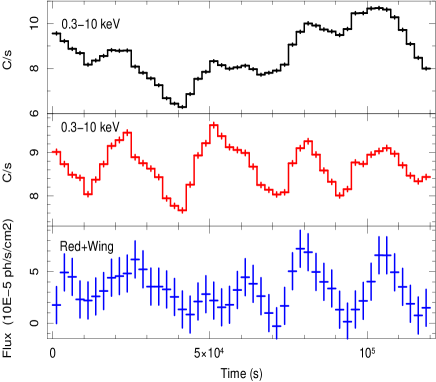
Figure 5: Upper panel: The 0.3–10 keV light curve of NGC 3783 during 2001b observation at 2.5 ks time resolution. Middle panel: The 0.3–10 keV light curve of NGC 3783 during the 2001b observation after subtraction of a 4th degree polynomial (long-term variations) at 2.5 ks time resolution. Lower panel: The 5.3–6.1 keV (“red+wing” energy band) light curve extracted from the excess emission map of the 2001b observation (Fig. 3, Right panel) at 2.5 ks time resolution.

Figure 6: The cross correlation function calculated between the de-trended 0.3–10 keV continuum light curve and the 5.3–6.1 keV feature (“red+wing”) light curve.

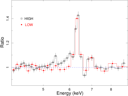
Figure 7: The Fe K line profile during the High flux (open squares) and the Low flux (solid circles) phases of the 5.3–6.1 keV feature. The ratios are computed against the best-fitting continuum model. The energies are in the observer frame.

6 Discussion

In the 2001b observation, NGC 3783 clearly exhibits continuum emission with two different time-scales: a long-term modulation with variations up to a factor 2 on intervals greater than 60 ks is superimposed to a shorter one on a time-scale of 27 ks, with modulations of 30% of the average value. According to an estimated black hole mass of $\mathrm{M_{BH}}=(3.0\pm 0.5)\times 10^{7}\leavevmode\nobreak\ \mathrm{M_{\odot}}$ (Peterson et al. peterson (2004)), the latter modulation occurs with a characteristic time-scale corresponding to the orbital period at $\sim$9–10 $\mathrm{r_{g}}$ (e.g. Bardeen, Press & Teukolsky (bardeen (1972))). It should be noted, however, that a previous mass estimate by Onken & Peterson (onken (2002)) gave the value of $\mathrm{M_{BH}}=(8.7\pm 1.1)\times 10^{6}\leavevmode\nobreak\ \mathrm{M_{\odot}}$, that would correspond to $\sim$20 $\mathrm{r_{g}}$. These mass discrepancies are mainly due to a different scaling of the virial relation in performing reverberation mapping measurements. However, the former estimate is more accurate because it has been calibrated to the $\mathrm{M_{BH}}-\sigma$ relation and thus we will adopt this value in the following discussion. The power spectral density of the source is consistent with a red-noise shape (Markowitz markowitz (2005)) where variability mainly occurs on intervals of the order of days. Here we identify an additional (additive) shorter time-scale component (see the footnote 1), most likely produced within the innermost accretion flow/corona system.

The most remarkable result of our analysis is the detection of redshifted (5.3–6.1 keV) Fe K emission and of its variability. The redshifted emission appears to respond only to the shorter $\sim$27 ks time-scale modulation and shows a good correlation with the continuum with a time-lag consistent with zero within the errors ($\Delta\tau\sim 1.25$ ks). This indicates that the continuum modulation on this time interval is likely to induce Fe K emission from dense material close to the black hole (which explains the observed redshift of the emission feature); moreover the lack of time-lags implies that the distance between the sites of continuum and line production is smaller than c$\Delta\tau\sim 4\times 10^{13}$ cm $\sim 8\leavevmode\nobreak\ \mathrm{r_{g}}$ (for the black hole mass given above). We are therefore most likely observing emission from the innermost accretion flow in both the continuum and line emission (corona and disc).

As discussed above, the variability time-scale suggests we are looking at emission from around $\sim$9–10 $\mathrm{r_{g}}$. As a consistency check, we fitted the time-averaged spectrum by including a diskline component to account for the redshifted features. We forced the emission region to be an annulus of $\Delta$r$=0.5\leavevmode\nobreak\ \mathrm{r_{g}}$ with uniform emissivity because the purpose of this test is to assess the approximate location of the line-emitting region. We obtain good fits with an almost face-on disc ($i=11\pm 4^{\circ}$) and an annulus at 9–15 $\mathrm{r_{g}}$ depending on the assumed Fe line rest-frame energy (from neutral at 6.4 keV to highly ionized at 6.97 keV). For all cases we tested, the statistical improvement is of $\Delta\chi^{2}\sim 16$ for 3 additional degrees of freedom, corresponding to a confidence level of 99.7%. This fit shows that the redshifted Fe line emission we detected is indeed consistent in shape with being produced around $10\leavevmode\nobreak\ \mathrm{r_{g}}$, where the disc orbital period is of the order of 27 ks, which agrees well with the correlated (and zero-lag) variability of the two components.

The interpretation of our results is however not straightforward. The quasi-sinusoidal modulations of the continuum and line emission (see Fig. 5) would suggest the presence of a localized co-rotating flare above the accretion disc which irradiates a small spot on its surface. The intensity modulations we see (Fig. 5) would then be produced by Doppler beaming effects (acting on both the flare and spot emission, i.e. on both continuum and line) and the characteristic time-scale of 27 ks would be identified with the orbital period (because of gravitational time dilation, the period measured by an observer on the disc at $10\leavevmode\nobreak\ \mathrm{r_{g}}$ would be shorter by $\sim$10%). As demonstrated above, a flare/spot system orbiting the black hole at $\sim$10 $\mathrm{r_{g}}$ would also produce a time-averaged line profile in agreement with the observations. However, such a model makes definite prediction on the Fe line energy modulation within one orbital period. In this framework, the orbiting spot on the accretion disc would also give rise to energy modulations of the Fe line due to the Doppler effect and such energy modulation is barely seen in the data (see Fig. 3). We stress that the adopted time resolution (2.5 ks) is good enough to detect energy modulations with a characteristic 27 ks time-scale. This has been demonstrated with XMM-Newton in the case of NGC 3516, where the modulation occurs on a very similar time-scale (Iwasawa et al. iwasawa2004 (2004); see also Dovčiak et al. dovciak (2004) for theoretical models). Therefore, the lack of Fe line energy modulation disfavours the orbiting flare/spot interpretation for NGC 3783.

However, a variability time-scale of the order of the orbital one at a given radius does not necessarily imply the motion of a point-like X-ray source. In fact, since the orbital time-scale is the fastest at a given disc radius, and since the observed time-scale of $\sim$27 ks corresponds to the orbital period at $\sim$10 $\mathrm{r_{g}}$, one could argue that the data only imply that the X-ray variability likely originates from within $\sim$10 $\mathrm{r_{g}}$. The apparent recurrence in the X-ray continuum modulation may not necessarily be related to a real physical periodicity, especially considering the limited length of the observation (only four putative cycles are detected).

A possible explanation for the observed behaviour is that the X-ray continuum source(s) (located within $\sim$10 $\mathrm{r_{g}}$ from the center) irradiates the whole accretion disc, but only a ring-like structure around $\mathrm{10\leavevmode\nobreak\ r_{g}}$ is responsible for the fluorescent Fe emission. This is possible if the bulk of the accretion disc is so highly ionized that little Fe line is produced, while an over-dense (and therefore lower ionization) structure is responsible for the fluorescent emission. Such an over-dense region could have an approximate ring-like geometry if it is for instance associated with a spiral-wave density perturbation. In this case, the Fe emitting region is extended in the azimuthal direction and we do not expect strong energy modulation with time, whatever the origin of the continuum modulation. We point out that spiral density distributions could result from the ordered magnetic fields in the inner region of the disc and that the energy dissipation (via e.g. magnetic reconnection) could be enhanced there, thereby providing a common site for the production of the X-ray continuum and the Fe line (e.g. Machida & Matsumoto machida (2003)).

On the other hand, if the apparent recurrence is in fact real, it is worth noting that the continuous theoretical effort in understanding the origin of quasi-periodic oscillations (QPO) in neutron star and black hole systems provides a wealth of mechanisms inducing quasi-periodic variability, although none is firmly established (Psaltis psaltis (2001); Kato kato (2001); Rezzolla et al. rezzolla (2003); Lee et al. lee (2004); Zycki & Sobolewska zycki (2005) and many others). A connection between QPO phase and Fe line intensity has been previously claimed in the Galactic black hole GRS 1915+105 (Miller & Homan miller2005 (2005)). Although in our case, the presence of a QPO cannot be claimed because of the very small number of detected cycles, the analogy is suggestive. In the case of GRS 1915+105, Miller & Homan consider that a warp in the inner disc, possibly due to Lense-Thirring precession, may produce the observed QPO-Fe line connection (e.g. Markovic & Lamb markovic (1998)). However, to produce the observed $\sim$15% rms variability in the X-ray lightcurve, the black hole spin axis should be inclined with respect to the line of sight by at least $60^{\circ}$ (which is at odds with our inclination estimate of $11\pm 4^{\circ}$ and with the Seyfert 1 nature of NGC 3783), and the tilt precession angle should be larger than 20^∘–30^∘ (Schnittman, Homan, Miller schnittman (2006)). Both requirements make it highly unlikely that Lense-Thirring precession can successfully account for the observed modulations in NGC 3783.

While the origin of the coherent intensity modulation still remains unclear, the correlated variation of the continuum and line emission and the Fe line shape are consistent with an emission site at $\sim$10 $\mathrm{r_{g}}$. Moreover, the fact that the iron line variability responds to the 27 ks time-scale modulation only implies that this short time-scale variation is somehow detached from the long-term variability. The latter may be associated with perturbations in the accretion disc propagating inwards from outer radii and modulating the X-ray emitting region (Lyubarskii lyubarskii (1997)), while the former seems to genuinely originate in the inner disc.

Further observational data may help to clarify the complex phenomena related to the relativistic Fe line temporal evolution in Seyfert 1 galaxies. Our work makes it clear that higher quality data in the Fe band will be able to probe the innermost regions of accretion flows with high accuracy. Next generation of large collecting area X-ray missions such as XEUS and Constellation-X or even very long observations with XMM-Newton will be crucial to fully exploit such potential.

- (1) Bardeen, J. M., Press, W. H., & Teukolsky, S. A. 1972, ApJ, 178, 347
- (2) Brenneman, L. W., & Reynolds, C. S. 2006, ArXiv Astrophysics e-prints, arXiv:astro-ph/0608502
- (3) De Rosa, A., Piro, L., Fiore, F. et al. 2002, A&A, 387, 838
- (4) De Marco, B., Cappi, M., Dadina, M., & Palumbo, G.G.C., 2006, Astron. Nach., astro-ph/0610882
- (5) Dovčiak, M., Bianchi, S., Guainazzi, M., Karas, V., & Matt, G. 2004, MNRAS, 350, 745
- (6) Fabian, A. C., Iwasawa, K., Reynolds, C. S., & Young, A. J. 2000, PASP, 112, 1145
- (7) Guainazzi, M., Bianchi, S., & Dovciak, M. 2006, ArXiv Astrophysics e-prints, arXiv:astro-ph/0610151
- (8) Iwasawa, K., et al. 1996, MNRAS, 282, 1038
- (9) Iwasawa, K., Miniutti, G., & Fabian, A. C. 2004, MNRAS, 355, 1073
- (10) Kaspi, S., et al. 2001, ApJ, 554, 216
- (11) Kato, S. 2001, PASJ, 53, L37
- (12) Lee W.H., Abramowicz M.A., & Kluzniak W., 2004, ApJ, 603, L93
- (13) Lyubarskii, Y. E. 1997, MNRAS, 292, 679
- (14) Machida, M., & Matsumoto, R. 2003, ApJ, 585, 429
- (15) Markovic D. & Lamb F.K., 1998, ApJ, 507, 316
- (16) Markowitz, A. 2005, ApJ, 635, 180
- (17) Miller J.M. & Homan J., 2005, ApJ, 618, L107
- (18) Miller, L., Turner, T. J., Reeves, J. N. et al. 2006, A&A, 453, L13
- (19) Miniutti, G., & Fabian, A. C. 2004, MNRAS, 349, 1435
- (20) Miniutti, G., et al. 2006, ArXiv Astrophysics e-prints, arXiv:astro-ph/0609521
- (21) Nandra, K., George, I. M., Mushotzky, R. F., Turner, T. J., & Yaqoob, T. 1997, ApJ, 477, 602
- (22) Nandra, K., O’Neill, P. M., George, I. M., Reeves, J. N., & Turner, T. J. 2006, ArXiv Astrophysics e-prints, arXiv:astro-ph/0610585
- (23) O’Neill, P. & Nandra, K., 2006, in preparation
- (24) Onken, C. A., & Peterson, B. M. 2002, ApJ, 572, 746
- (25) Peterson, B. M., et al. 2004, ApJ, 613, 682
- (26) Ponti, G., Cappi, M., Dadina, M., & Malaguti, G. 2004, A&A, 417, 451
- (27) Psaltis D., 2001, Adv Space Res., 28, 481
- (28) Reeves, J. N., Nandra, K., George, I. M. et al. 2004, ApJ, 602, 648
- (29) Reynolds, C. S., & Nowak, M. A. 2003, Phys. Rep, 377, 389
- (30) Rezzolla L., Yoshida S., Maccarone T.J., Zanotti O., 2003, MNRAS, 344, L37
- (31) Schnittman J.D., Homan J., Miller J.M., 2006, ApJ, 642, 420
- (32) Turner, T. J., Miller, L., George, I. M., & Reeves, J. N. 2006, A&A, 445, 59
- (33) Vaughan, S., & Edelson, R. 2001, ApJ, 548, 694
- (34) Zycki P.T. & Sobolewska M.A., 2005, MNRAS, 364, 891