Curvature and isocurvature perturbations
in two-field inflation

Abstract

We study cosmological perturbations in two-field inflation, allowing for non-standard kinetic terms. We calculate analytically the spectra of curvature and isocurvature modes at Hubble crossing, up to first order in the slow-roll parameters. We also compute numerically the evolution of the curvature and isocurvature modes from well within the Hubble radius until the end of inflation. We show explicitly for a few examples, including the recently proposed model of ‘roulette’ inflation, how isocurvature perturbations affect significantly the curvature perturbation between Hubble crossing and the end of inflation.

1 Introduction

Inflation provides a simple and elegant scenario for the early Universe (see e.g. [1] for a recent textbook presentation). Although single field inflation models are perfectly compatible with the present cosmological data, many early universe models based on high energy physics, in particular derived from supergravity or string theory, usually involve many scalar fields which can have non-standard kinetic terms. This is why multi-field inflationary scenarios, where several scalar fields play a dynamical role during inflation, have received some attention in the literature (see e.g. [2]-[13]). However, except for a few specific models, the predictions for the spectra of primordial perturbations are, in general, a nontrivial task, in contrast with single-field models.

The main reason is that the curvature (or adiabatic) perturbation, which is generated during inflation and eventually observed, can evolve on super-Hubble scales in multi-field inflation whereas it remains frozen in single-field inflation. This is due to the presence of additional perturbation modes, often called isocurvature (or entropy) modes, corresponding to relative perturbations between the various scalar fields, which act as a source term in the evolution equation for the curvature perturbation. This property was first pointed out in [6] in the context of Brans-Dicke inflation. This phenomenon occurs during inflation and affects the final curvature perturbation at the end of inflation, independently whether isocurvature modes survive or not after inflation.

The purpose of the present work is to study in detail how the isocurvature perturbations, present during inflation, affect the curvature perturbations, both at Hubble crossing and in the subsequent evolution on super-Hubble scales. Since our intention is to stress some qualitative properties specific to multi-field inflation, we have chosen to restrict our study to the case of two scalar fields. Moreover, we consider models where a non-standard kinetic term is allowed for one of the scalar fields. This includes, in particular, scenarios motivated by supergravity and string theory, which have been recently proposed (see, e.g., [14]-[18]).

The production of adiabatic and isocurvature modes for two-field inflation with a generic potential, in the slow-roll approximation, was studied in [19] where a decomposition into adiabatic and isocurvature modes was introduced. Models with non-standard kinetic terms for inflatons have been studied in the slow-roll approximation in [9] and [11], and the adiabatic-isocurvature decomposition technique of [19] was later extended to such two-field models in [20] and [21]. Very recently, two-field inflation with standard kinetic terms was investigated in [22] at next-to-leading order correction in a slow-roll expansion and it was also shown that the adiabatic and isocurvature modes at Hubble crossing are correlated at first order in slow-roll parameters. In parallel to these analytical studies, a numerical study of the evolution of adiabatic and isocurvature was presented in [23] and [24].

In the present work, we extend the previous analyses in the following directions. First, we present a detailed analysis of the correlation of adiabatic and isocurvature just after Hubble crossing, both analytically and numerically. This correlation was in general supposed to vanish in most previous works, except in the numerical study [23] and the analytical work [22], both in the context of canonical kinetic terms. Here, we extend the analysis with non-standard kinetic terms. We compute analytically the spectra and correlation at Hubble crossing in the slow-roll approximation, by taking special care of the time-dependence shortly after Hubble crossing.

Second, we study numerically the whole evolution of adiabatic and isocurvature perturbations from within the Hubble radius until the end of inflation. This allows us to go beyond the slow-roll approximation which is needed to derive analytical results. Our numerical study enables us to see precisely how isocurvature perturbations can be transferred into adiabatic perturbations during the inflationary phase depending on the background trajectory in field space. We illustrate this behaviour by studying numerically three models. The last one is the so-called ’roulette’ inflation model, which has been proposed recently [14].

The plan of the paper is the following. The next section presents the class of models we consider and gives the homogeneous equations of motion as well as the equations governing the perturbations. The third section is devoted to the study of the perturbations from deep inside the Hubble radius until a few e-folds after Hubble crossing. We then discuss, in section 4, analytical methods to determine the evolution of the perturbations on super-Hubble scales. Section 5 is devoted to the numerical study of the evolution of the perturbations, which is compared with the analytical estimates of the previous sections. We finally draw our conclusions in the last section.

2 The model

In this paper, we study models with two scalar fields, in which one of the scalar fields has a non-standard kinetic term, described by an action of the form

$$S=\int d^{4}x\sqrt{-g}\left[\frac{M_{P}^{2}}{2}R-\frac{1}{2}(\partial_{\mu}\phi)(\partial^{\mu}\phi)-\frac{e^{2b(\phi)}}{2}(\partial_{\mu}\chi)(\partial^{\mu}\chi)-V(\phi,\chi)\right],$$ (1)

where ${M_{P}}$ is the reduced Planck mass, ${M_{P}}\equiv(8\pi G)^{-1/2}$. This type of action usually appears when $\chi$ corresponds to an axionic component. It is also motivated by generalized Einstein theories [6, 11]. When $b(\phi)=0$ one recovers standard kinetic terms for the two fields. In this section, we give the equations of motion for the homogeneous fields and then for the linear perturbations, following the results (and notation) of [20] and [21], where the same type of models was considered.

2.1 Homogeneous equations

Let us start with the homogeneous equations of motion. We assume a spatially flat FLRW (Friedmann-Lemaître-Robertson-Walker) geometry, with metric

$$ds^{2}=-dt^{2}+a(t)^{2}d{\bf x}^{2},$$ (2)

where $t$ is the cosmic time. One can also define the comoving time $\tau=\int dt/a(t)$.

The equations of motion for the scale factor and the homogeneous fields read

$$\ddot{\phi}+3H\dot{\phi}+V_{\phi}=b_{\phi}e^{2b}\dot{\chi}^{2}\,,$$ (3)

$$\ddot{\chi}+(3H+2b_{\phi}\dot{\phi})\dot{\chi}+e^{-2b}\,V_{\chi}=0\,,$$ (4)

$$H^{2}=\frac{1}{3M_{P}^{2}}\left[\frac{1}{2}\dot{\phi}^{2}+\frac{e^{2b}}{2}\dot{\chi}^{2}+V\right]\,,$$ (5)

and

$$\dot{H}=-\frac{1}{2M_{P}^{2}}\left[\dot{\phi}^{2}+e^{2b}\dot{\chi}^{2}\right]\,,$$ (6)

where $H\equiv\dot{a}/a$ and a dot stands for a derivative with respect to the cosmic time $t$ and a subscript index $\phi$ or $\chi$ denotes a derivative with respect to the corresponding field.

It is also useful to introduce the following slow-roll parameters

$$\epsilon_{\phi\phi}=\frac{\dot{\phi}^{2}}{2M_{P}^{2}H^{2}},\quad\epsilon_{\phi\chi}=e^{b}\frac{\dot{\phi}\dot{\chi}}{2M_{P}^{2}H^{2}},\quad\epsilon_{\chi\chi}=e^{2b}\frac{\dot{\chi}^{2}}{2M_{P}^{2}H^{2}},$$ (7)

$$\eta_{IJ}=\frac{V_{IJ}}{3H^{2}}$$ (8)

and

$$\epsilon=\epsilon_{\phi\phi}+\epsilon_{\chi\chi}=-\frac{\dot{H}}{H^{2}}.$$ (9)

2.2 Linear perturbations

We now discuss the linear perturbations of our model (one can find a detailed presentation of the theory of cosmological perturbations in e.g. [1, 25, 26] and a pedagogical introduction in e.g. [27]). For simplicity, we shall directly work in the longitudinal gauge. In the absence of anistropic stress (the off-diagonal spatial components of the stress-energy tensor), which is the case when matter consists of scalar fields, the metric in the longitudinal gauge is of the form

$$\mathrm{d}s^{2}=-(1+2\Phi)\mathrm{d}t^{2}+a^{2}(1-2\Phi)\mathrm{d}{\bf x}^{2}\,.$$ (10)

where only scalar perturbations are taken into account.

We now decompose the scalar fields into their homogeneous (background) parts and the perturbations:

$$\phi(t,{\bf x})=\phi(t)+\delta\phi(t,{\bf x})\qquad\textrm{and}\qquad\chi(t,{\bf x})=\chi(t)+\delta\chi(t,{\bf x})\,.$$ (11)

We shall work with the Fourier components of the perturbations, $\delta\phi_{\mathbf{k}}(t)$ and $\delta\chi_{\mathbf{k}}(t)$, routinely omitting the subscript $\mathbf{k}$ to shorten the expressions. The perturbed Klein-Gordon equations read

$$\ddot{\delta\phi} + 3H\dot{\delta\phi}+\left[\frac{k^{2}}{a^{2}}+V_{\phi\phi}-(b_{\phi\phi}+2b_{\phi}^{2})\dot{\chi}^{2}e^{2b}\right]\delta\phi+V_{\phi\chi}\delta\chi-2b_{\phi}e^{2b}\dot{\chi}\dot{\delta\chi}$$ (12)

$$= 4\dot{\phi}\dot{\Phi}-2V_{\phi}\Phi\,$$

and

$$\ddot{\delta\chi} + (3H+2b_{\phi}\dot{\phi})\dot{\delta\chi}+\left[\frac{k^{2}}{a^{2}}+e^{-2b}V_{\chi\chi}\right]\delta\chi+2b_{\phi}\dot{\chi}\,\dot{\delta\phi}+$$ (13)

$$+ \left[e^{-2b}\left(V_{\chi\phi}-2b_{\phi}V_{\chi}\right)+2b_{\phi\phi}\dot{\phi}\dot{\chi}\right]\delta\phi=4\dot{\chi}\dot{\Phi}-2e^{-2b}V_{\chi}\Phi\,.$$

The energy and the momentum constraints, given by Einstein equations, are, respectively:

$$3H(\dot{\Phi}+H\Phi)+\dot{H}\Phi+\frac{k^{2}}{a^{2}}\Phi=-\frac{1}{2M_{P}^{2}}\left[\dot{\phi}\,\dot{\delta\phi}+e^{2b}\dot{\chi}\,\dot{\delta}\chi+b_{\phi}e^{2b}\dot{\chi}^{2}\delta\phi+V_{\phi}\delta\phi+V_{\chi}\delta\chi\right]$$ (14)

$$\dot{\Phi}+H\Phi=\frac{1}{2M_{P}^{2}}\left(\dot{\phi}\,\delta\varphi+e^{2b}\dot{\chi}\,\delta\chi\right)\,\,.$$ (15)

It is convenient, instead of using the perturbations $\delta\phi$ and $\delta\chi$, defined here in the longitudinal gauge, to introduce the so-called gauge-invariant Mukhanov-Sasaki variables:

$$Q_{\phi}\equiv\delta\phi+\frac{\dot{\phi}}{H}\Phi\qquad\textrm{and}\qquad Q_{\chi}\equiv\delta\chi+\frac{\dot{\chi}}{H}\Phi\,,$$ (16)

which can be identified with the scalar field perturbations in the flat gauge.

Substituting (16) into (12)-(13) and using the background equations of motion as well as the energy and momentum constraints, one finds

$$\ddot{Q}_{\phi}+3H\dot{Q}_{\phi}-2e^{2b}b_{\phi}\,\dot{\chi}\,\dot{Q}_{\chi}+\left(\frac{k^{2}}{a^{2}}+C_{\phi\phi}\right)Q_{\phi}+C_{\phi\chi}Q_{\chi}=0$$ (17)

$$\ddot{Q}_{\chi}+3H\dot{Q}_{\chi}+2b_{\phi}\,\dot{\phi}\,\dot{Q}_{\chi}+2b_{\phi}\,\dot{\chi}\,\dot{Q}_{\phi}+\left(\frac{k^{2}}{a^{2}}+C_{\chi\chi}\right)Q_{\chi}+C_{\chi\phi}Q_{\phi}=0\,,$$ (18)

where we have defined the following background-dependent coefficients:

$$C_{\phi\phi} = -2e^{2b}b_{\phi}^{2}\dot{\chi}^{2}+\frac{3\dot{\phi}^{2}}{M_{P}^{2}}-\frac{e^{2b}\dot{\phi}^{2}\dot{\chi}^{2}}{2M_{P}^{4}H^{2}}-\frac{\dot{\phi}^{4}}{2M_{P}^{4}H^{2}}-e^{2b}b_{\phi\phi}\dot{\chi}^{2}+\frac{2\dot{\phi}V_{\phi}}{M_{P}^{2}H}+V_{\phi\phi}$$ (19)

$$C_{\phi\chi} = \frac{3e^{2b}\dot{\phi}\dot{\chi}}{M_{P}^{2}}-\frac{e^{4b}\dot{\phi}\dot{\chi}^{3}}{2M_{P}^{4}H^{2}}-\frac{e^{2b}\dot{\phi}^{3}\dot{\chi}}{2M_{P}^{4}H^{2}}+\frac{\dot{\phi}V_{\chi}}{M_{P}^{2}H}+\frac{e^{2b}\dot{\chi}V_{\phi}}{M_{P}^{2}H}+V_{\phi\chi}$$ (20)

$$C_{\chi\chi} = \frac{3e^{2b}\dot{\chi}^{2}}{M_{P}^{2}}-\frac{e^{4b}\dot{\chi}^{4}}{2M_{P}^{4}H^{2}}-\frac{e^{2b}\dot{\phi}^{2}\dot{\chi}^{2}}{2M_{P}^{4}H^{2}}+\frac{2\dot{\chi}V_{\chi}}{M_{P}^{2}H}+e^{-2b}V_{\chi\chi}$$ (21)

$$C_{\chi\phi} = \frac{3\dot{\phi}\dot{\chi}}{M_{P}^{2}}-\frac{e^{2b}\dot{\phi}\dot{\chi}^{3}}{2M_{P}^{4}H^{2}}-\frac{\dot{\phi}^{3}\dot{\chi}}{2M_{P}^{4}H^{2}}+2b_{\phi\phi}\dot{\phi}\dot{\chi}-2e^{-2b}b_{\phi}V_{\chi}+$$ (22)

$$+\frac{e^{-2b}\dot{\phi}V_{\chi}}{M_{P}^{2}H}+\frac{\dot{\chi}V_{\phi}}{M_{P}^{2}H}+e^{-2b}V_{\phi\chi}$$

The two equations (17) and (18) form a closed system for the two gauge-invariant quantities $Q_{\phi}$ and $Q_{\chi}$.

2.3 Decomposition into adiabatic and entropy components

As originally proposed in [19], in order to facilitate the interpretation of the evolution of cosmological perturbations, it can be useful to decompose the scalar field perturbations along the two directions respectively parallel and orthogonal to the homogeneous trajectory in field space. The projection parallel to the trajectory is usually called the adiabatic, or curvature, component while the orthogonal projection corresponds to the entropy, or isocurvature, component. Note that there was a semantic shift in the terminology since one used to call adiabatic and entropy modes during inflation the two particular solutions for the perturbations that would match after inflation, respectively, to the adiabatic and isocurvature modes defined in the radiation era. This terminology is used for example in the papers on double inflation such that [5] and [10].

This decomposition into instantaneous adiabatic and entropy components, introduced in [19], has recently been extended [28] to fully nonlinear perturbations in the context of the covariant nonlinear formalism introduced in [29, 30]. Here, we consider only the decomposition at the linear level, but since we allow for non-standard kinetic terms, we will need to generalize the equations to such a case, as was done in [20]. Let us recall here the main results.

The essential idea is to introduce the linear combinations

$$\delta\sigma\equiv\cos\theta\,\delta\phi+\sin\theta\,e^{b}\,\delta\chi\qquad\textrm{and}\qquad\delta s\equiv-\sin\theta\,\delta\phi+\cos\theta\,e^{b}\,\delta\chi\,,$$ (23)

where

$$\cos\theta\equiv\frac{\dot{\phi}}{\dot{\sigma}},\qquad\sin\theta\equiv\frac{\dot{\chi}\,e^{b}}{\dot{\sigma}}\qquad\textrm{with}\qquad\dot{\sigma}\equiv\sqrt{\dot{\phi}^{2}+e^{2b}\dot{\chi}^{2}}\,.$$ (24)

The notations $\dot{\sigma}$ and $\delta\sigma$ are just used for convenience; they do not refer to any scalar field $\sigma$.

Instead of $\delta\sigma$, it is in fact more convenient to work directly with the Mukhanov-Sasaki variables and therefore to define

$$Q_{\sigma}\equiv\cos\theta\,Q_{\phi}+\sin\theta\,e^{b}\,Q_{\chi}\qquad\textrm{and}\qquad\delta s\equiv-\sin\theta\,Q_{\phi}+\cos\theta\,e^{b}\,Q_{\chi}\,,$$ (25)

by noting that

$$Q_{\sigma}\equiv\delta\sigma+\frac{\dot{\sigma}}{H}\Phi.$$ (26)

In the so-called comoving gauge, the perturbation $Q_{\sigma}$ is directly related to the three-dimensional curvature of the constant time space-like slices. This gives the gauge-invariant quantity refered to as the comoving curvature perturbation:

$$\mathcal{R}\equiv\frac{H}{\dot{\sigma}}Q_{\sigma}.$$ (27)

The perturbation $\delta s$, called the isocurvature perturbation, is automatically gauge-invariant. It is sometimes convenient, by analogy with the curvature perturbation, to introduce a renormalized entropy perturbation which is defined as

$$\mathcal{S}\equiv\frac{H}{\dot{\sigma}}\delta s.$$ (28)

In field space, $Q_{\sigma}$ corresponds to perturbations parallel to the velocity vector $(\dot{\phi},e^{b}\dot{\chi})$, while $\delta s$ to the orthogonal ones.

Introducing the adiabatic and entropy “vectors” in field space, respectively

$$E_{\sigma}^{I}=\left(\cos\theta,e^{-b}\sin\theta\right),\qquad E_{s}^{I}=\left(-\sin\theta,e^{-b}\cos\theta\right),\qquad I=\left\{\phi,\chi\right\},$$ (29)

one can define various derivatives of the potential with respect to the adiabatic and entropy directions. Assuming an implicit summation on the indices $I$ (and $J$), the first order derivatives are defined as

$$V_{\sigma}=E_{\sigma}^{I}V_{I},\qquad V_{s}=E_{s}^{I}V_{I},$$ (30)

whereas the second order derivatives are

$$V_{\sigma\sigma}=E_{\sigma}^{I}E_{\sigma}^{J}V_{IJ},\quad V_{\sigma s}=E_{\sigma}^{I}E_{s}^{J}V_{IJ},\quad V_{ss}=E_{s}^{I}E_{s}^{J}V_{IJ}.$$ (31)

By combining the two Klein-Gordon equations for the background fields, (3) and (4), one gets the background equations of motion along the adiabatic and entropy directions, respectively,

$$\ddot{\sigma}+3H\dot{\sigma}+V_{\sigma}=0,$$ (32)

$$\dot{\theta}=-\frac{V_{s}}{\dot{\sigma}}-b_{\phi}\dot{\sigma}\sin\theta,$$ (33)

while the equations of motion for the perturbations read:

$$\ddot{Q}_{\sigma}+3H\dot{Q}_{\sigma}+\left(\frac{k^{2}}{a^{2}}+C_{\sigma\sigma}\right)Q_{\sigma}+\frac{2V_{s}}{\dot{\sigma}}\dot{\delta s}+C_{\sigma s}\,\delta s=0$$ (34)

$$\ddot{\delta s}+3H\dot{\delta s}+\left(\frac{k^{2}}{a^{2}}+C_{ss}\right)\delta s-\frac{2V_{s}}{\dot{\sigma}}\dot{Q}_{\sigma}+C_{s\sigma}Q_{\sigma}=0\,,$$ (35)

with

$$C_{\sigma\sigma} = V_{\sigma\sigma}-\left(\frac{V_{s}}{\dot{\sigma}}\right)^{2}+2\frac{\dot{\sigma}V_{\sigma}}{M_{P}^{2}H}+\frac{3\dot{\sigma}^{2}}{M_{P}^{2}}-\frac{\dot{\sigma}^{4}}{2M_{P}^{4}H^{2}}-b_{\phi}\left(s_{\theta}^{2}c_{\theta}V_{\sigma}+(c_{\theta}^{2}+1)s_{\theta}V_{s}\right)$$ (36)

$$C_{\sigma s} = 6H\frac{V_{s}}{\dot{\sigma}}+\frac{2V_{\sigma}V_{s}}{\dot{\sigma}^{2}}+2V_{\sigma s}+\frac{\dot{\sigma}V_{s}}{M_{P}^{2}H}+2b_{\phi}(s_{\theta}^{3}V_{\sigma}-c_{\theta}^{3}V_{s})$$ (37)

$$C_{ss} = V_{ss}-\left(\frac{V_{s}}{\dot{\sigma}}\right)^{2}+b_{\phi}(1+s_{\theta}^{2})c_{\theta}V_{\sigma}+b_{\phi}c_{\theta}^{2}s_{\theta}V_{s}-\dot{\sigma}^{2}(b_{\phi\phi}+b_{\phi}^{2})$$ (38)

$$C_{s\sigma} = -6H\frac{V_{s}}{\dot{\sigma}}-\frac{2V_{\sigma}V_{s}}{\dot{\sigma}^{2}}+\frac{\dot{\sigma}V_{s}}{M_{P}^{2}H}$$ (39)

where $s_{\theta}\equiv\sin\theta$ and $c_{\theta}\equiv\cos\theta$.

The above system consists (34-35) of two coupled second order differential equations involving only $Q_{\sigma}$ and $\delta s$. In order to relate these variables to the metric perturbation $\Phi$ defined in the longitudinal gauge, it is useful to use the Poisson-like constraint, which follows from the energy and momentum constraints (14) and (15),

$$\frac{k^{2}}{a^{2}}\Phi=-\frac{1}{2M_{P}^{2}}\epsilon_{m}$$ (40)

where $\epsilon_{m}$ is the comoving energy density and can be expressed as

$$\epsilon_{m}=\dot{\sigma}\dot{Q}_{\sigma}+\left(3H+\frac{\dot{H}}{H}\right)\dot{\sigma}Q_{\sigma}+V_{\sigma}Q_{\sigma}+2V_{s}\delta s.$$ (41)

2.4 Perturbation spectra

The inflationary observables are customarily expressed in terms of power spectra and correlation functions. Given their origin as quantum fluctuations, the perturbations can be represented as random variables. We introduce the power spectra of the adiabatic and entropy perturbations, respectively

$$\langle{Q_{\sigma}}^{\ast}_{\mathbf{k}}\,{Q_{\sigma}}_{\mathbf{k}^{\prime}}\rangle=\frac{2\pi^{2}}{k^{3}}\mathcal{P}_{Q_{\sigma}}(k)\delta(\mathbf{k}-\mathbf{k}^{\prime}),\quad\langle\delta s^{\ast}_{\mathbf{k}}\,\delta s_{\mathbf{k}^{\prime}}\rangle=\frac{2\pi^{2}}{k^{3}}\mathcal{P}_{\delta s}(k)\delta(\mathbf{k}-\mathbf{k}^{\prime}),$$ (42)

as well as the correlation spectrum

$$\langle{Q_{\sigma}}^{\ast}_{\mathbf{k}}\,\delta s_{\mathbf{k}^{\prime}}\rangle=\frac{2\pi^{2}}{k^{3}}\mathcal{C}_{Q_{\sigma}\,\delta s}(k)\delta(\mathbf{k}-\mathbf{k}^{\prime}).$$ (43)

3 Evolution of perturbations inside the Hubble radius

In order to study the generation of perturbations from vacuum fluctuations, we start, for a given comoving wave number $k$, at an instant $t_{i}$ (or $\tau_{i}$) during inflation when the physical wave number $k/a$ is much bigger than the Hubble parameter $H$. Our initial conditions are given, as usual, by the Minkowski-like vacuum at $\tau_{i}$,

$$Q_{\sigma}(\tau_{i})\simeq\frac{e^{-\imath k\tau_{i}}}{a(\tau_{i})\sqrt{2k}}\qquad\textrm{and}\qquad\delta s(\tau_{i})\simeq\frac{e^{-\imath k\tau_{i}}}{a(\tau_{i})\sqrt{2k}}$$ (44)

for initial adiabatic and isocurvature fluctuations, respectively. These two initial fluctuations are statistically independent because the corresponding equations of motion are decoupled in the limit $k\gg aH$.

Although the adiabatic and entropy fluctuations are initially, i.e. deep inside the Hubble radius, statistically independent, this is, in general, no longer the case at Hubble crossing. In the context of two-field inflation with canonical kinetic terms, this point has been stressed in the numerical analysis of [23] and studied analytically in [22].

In the following, we extend the analysis of [22] to non-canonical kinetic terms.

3.1 Equations in the slow-roll approximation

We start with the perturbations $Q_{\sigma}$ and $\delta s$, whose dynamics is described by eqs. (34) and (35). Using the conformal time $\tau$ and introducing the variables

$$u_{\sigma}=a\,Q_{\sigma},\qquad u_{s}=a\,\delta s,$$ (45)

these equations can be rewritten in the form

$$u_{\sigma}^{\prime\prime}+\frac{2V_{s}}{\dot{\sigma}}au_{s}^{\prime}+\left[k^{2}-\frac{a^{\prime\prime}}{a}+a^{2}{C}_{\sigma\sigma}\right]u_{\sigma}+\left[-\frac{2V_{s}}{\dot{\sigma}}a^{\prime}+a^{2}{C}_{\sigma s}\right]u_{s}=0,$$ (46)

$$u_{s}^{\prime\prime}-\frac{2V_{s}}{\dot{\sigma}}au_{\sigma}^{\prime}+\left[k^{2}-\frac{a^{\prime\prime}}{a}+a^{2}{C}_{ss}\right]u_{s}+\left[\frac{2V_{s}}{\dot{\sigma}}a^{\prime}+a^{2}{C}_{s\sigma}\right]u_{\sigma}=0,$$ (47)

where the four coefficients ${C}_{IJ}$ are given in eqs. (36)-(39) and a prime denotes a derivative with respect to the conformal time $\tau$.

Let us now discuss the slow-roll approximation. The only difference with respect to the case with canonical kinetic terms will arise from some of the terms depending on the derivatives of $b$. In the slow-roll approximation, one can use the relation

$$\frac{V_{s}}{\dot{\sigma}}=H\eta_{\sigma s}-b_{\phi}\dot{\sigma}s_{\theta}^{3}\,,$$ (48)

and the various coefficients in the above system of equations simplify to yield

$$\left[\left(\frac{\mathrm{d}^{2}{}}{\mathrm{d}\tau^{2}}+k^{2}-\frac{2+3\epsilon}{\tau^{2}}\right)\mathbf{1}+2\mathbf{E}\frac{1}{\tau}\frac{\mathrm{d}{}}{\mathrm{d}\tau}+\mathbf{M}\frac{1}{\tau^{2}}\right]\left(\begin{array}[]{c}u_{\sigma}\\ u_{s}\end{array}\right)=0\,$$ (49)

where the matrices $\mathbf{E}$ and $\mathbf{M}$ are given by

$$\mathbf{E} = \left(\begin{array}[]{cc}0&-\eta_{\sigma s}\\ \eta_{\sigma s}&0\end{array}\right)+\left(\begin{array}[]{cc}0&\xi s_{\theta}^{3}\\ -\xi s_{\theta}^{3}&0\end{array}\right)$$ (54)

$$\mathbf{M} = \left(\begin{array}[]{cc}-6\epsilon+3\eta_{\sigma\sigma}&4\eta_{\sigma s}\\ 2\eta_{\sigma s}&3\eta_{ss}\end{array}\right)+\left(\begin{array}[]{cc}3\xi s_{\theta}^{2}c_{\theta}&-4\xi s_{\theta}^{3}\\ -2\xi s_{\theta}^{3}&-3\xi c_{\theta}(1+s_{\theta}^{2})\end{array}\right)$$ (59)

with

$$\xi\equiv\sqrt{2}b_{\phi}M_{P}\sqrt{\epsilon}.$$ (60)

In eqs. (54) and (59), we have kept only the terms linear in $b_{\phi}$, i.e. proportional to $\xi$, and neglected the terms quadratic in $b_{\phi}$ as well as the terms proportional to $b_{\phi\phi}$. We thus treat $\xi$ on the same footing as the other slow-roll parameters. In order to emphasize the difference between generalized kinetic terms and canonical kinetic terms, we have however separated the terms proportional $\xi$ from the others.

The system of equations (49) that we have obtained is of the form

$$u^{\prime\prime}+2\mathbf{L}u^{\prime}+\mathbf{Q}u=0\,.$$ (61)

The matrix coefficient for the first order time derivative is $2\mathbf{L}=2\mathbf{E}/\tau$, where $\mathbf{E}$ is an antisymmetric matrix, linear in the slow-roll parameters. Let us introduce a time-dependent orthogonal matrix $\mathbf{R}$ which satisfies $\mathbf{R}^{\prime}=-\mathbf{L}\mathbf{R}$. Note that this is possible only if $\mathbf{L}$ is an antisymmetric matrix. Reexpressing the above equation (61) in terms of a new matrix vector $v$, defined by $u=\mathbf{R}v$, one can eliminate the terms proportional to the first order time derivative and we obtain the following equation

$$v^{\prime\prime}+\mathbf{R}^{-1}\left(-\mathbf{L}^{2}-\mathbf{L}^{\prime}+\mathbf{Q}\right)\mathbf{R}v=0.$$ (62)

At linear order in the slow-roll parameters, one finds

$$-\mathbf{L}^{2}-\mathbf{L}^{\prime}\simeq\frac{1}{\tau^{2}}\mathbf{E}.$$ (63)

Therefore, apart from the trivial part proportional to the identity matrix, the combination $-\mathbf{L}^{2}-\mathbf{L}^{\prime}+\mathbf{Q}$ contains

$$\frac{1}{\tau^{2}}(\mathbf{E}+\mathbf{M})=\frac{3}{\tau^{2}}\left(\begin{array}[]{cc}-2\epsilon+\eta_{\sigma\sigma}+\xi s_{\theta}^{2}c_{\theta}&\eta_{\sigma s}-\xi s_{\theta}^{3}\\ \eta_{\sigma s}-\xi s_{\theta}^{3}&\eta_{ss}-\xi c_{\theta}(1+s_{\theta}^{2})\end{array}\right)\,,$$ (64)

which is a symmetric matrix.

We now assume that the slow-roll parameters vary sufficiently slowly during the few e-folds when the given scale crosses out the Hubble radius. We thus replace the time-dependent matrix on the right hand side of (64) by the same matrix evaluated at Hubble crossing, i.e. for $k=aH$, and the only remaining time dependence appears in the global coefficient $3/\tau^{2}$. One can now diagonalize this matrix by introducing the time-independent rotation matrix

$$\mathbf{\tilde{R}}_{*}=\left(\begin{array}[]{cc}\cos\Theta_{*}&-\sin\Theta_{*}\\ \sin\Theta_{*}&\cos\Theta_{*}\end{array}\right),$$ (65)

so that

$$\mathbf{\tilde{R}}_{*}^{-1}\left(\mathbf{M}+\mathbf{E}\right)\mathbf{\tilde{R}}_{*}={\rm Diag}(\tilde{\lambda}_{1},\tilde{\lambda}_{2}).$$ (66)

In particular, one can easily compute the following linear combinations, which will be useful later:

$$\tilde{\lambda}_{1}+\tilde{\lambda}_{2}=3\left(\eta_{\sigma\sigma}+\eta_{ss}-2\epsilon-\xi c_{\theta}\right),$$ (67)

$$(\tilde{\lambda}_{1}-\tilde{\lambda}_{2})\sin 2\Theta_{*}=6\left(\eta_{\sigma s}-\xi s_{\theta}^{3}\right),$$ (68)

$$(\tilde{\lambda}_{1}-\tilde{\lambda}_{2})\cos 2\Theta_{*}=3\left(\eta_{\sigma\sigma}-\eta_{ss}-2\epsilon+\xi c_{\theta}(1+2s_{\theta}^{2})\right),$$ (69)

where the right hand sides of the three above equations are evaluated at $k=aH$.

Similarly, the rotation matrix $\mathbf{R}$ is slowly varying per efold, since $(\mathrm{d}\mathbf{R}/\mathrm{d}\,\ln a)\mathbf{R}^{T}=\mathbf{E}$, where $\mathbf{E}$ is linear in slow-roll parameters. Around Hubble crossing, one can thus replace $\mathbf{R}$ by its value $\mathbf{R}_{*}$ at Hubble crossing.

By introducing

$$w=\mathbf{\tilde{R}}_{*}^{-1}\mathbf{R}_{*}v,$$ (70)

the system of equations can be written as two independent equations of the form

$$w_{A}^{\prime\prime}+\left[k^{2}-\frac{1}{\tau^{2}}\left(2+3\lambda_{A}\right)\right]w_{A}=0,\qquad\left(A=1,2\right)$$ (71)

with

$$\lambda_{A}=\epsilon-\frac{1}{3}\tilde{\lambda}_{A}.$$ (72)

Defining

$$\mu_{A}=\sqrt{\frac{9}{4}+3\lambda_{A}}$$ (73)

the solution of (71) with the proper asymptotic behaviour can be written as

$$w_{A}=\frac{\sqrt{\pi}}{2}e^{i(\mu_{A}+1/2)\pi/2}\sqrt{-\tau}H_{\mu_{A}}^{(1)}(-k\tau)e_{A}(k),$$ (74)

where $H_{\mu}^{(1)}$ is the Hankel function of the first kind of order $\mu$ and the $e_{A}$ are two independent normalized Gaussian random variables so that

$$\langle e_{A}(k)\rangle=0,\qquad\langle e_{A}(k)e_{B}^{*}(k^{\prime})\rangle=\delta_{AB}\delta^{(3)}(k-k^{\prime}).$$ (75)

Using the independence of the variables $w_{1}$ and $w_{2}$, one can express the correlations for the variables $u_{\sigma}$ and $u_{s}$ around Hubble crossing time as

$$a^{2}\langle Q_{\sigma}^{\dagger}Q_{\sigma}\rangle = \cos^{2}\Theta_{*}\langle w_{1}^{\dagger}w_{1}\rangle+\sin^{2}\Theta_{*}\langle w_{2}^{\dagger}w_{2}\rangle$$ (76)

$$a^{2}\langle\delta s^{\dagger}Q_{\sigma}\rangle = \frac{1}{2}\sin 2\Theta_{*}\left(\langle w_{1}^{\dagger}w_{1}\rangle-\langle w_{2}^{\dagger}w_{2}\rangle\right)$$ (77)

$$a^{2}\langle\delta s^{\dagger}\delta s\rangle = \sin^{2}\Theta\langle w_{1}^{\dagger}w_{1}\rangle+\cos^{2}\Theta\langle w_{2}^{\dagger}w_{2}\rangle$$ (78)

where one can substitute

$$\langle w_{A}^{\dagger}w_{A}\rangle=\frac{\pi}{4}(-\tau)|H^{(1)}_{\mu_{A}}(-k\tau)|^{2}\equiv\frac{1}{2k}\frac{1}{(k\tau)^{2}}{\cal F}_{A}(-k\tau).$$ (79)

This yields

$${\cal P}_{Q_{\sigma}} = \left(\frac{H_{*}}{2\pi}\right)^{2}(1-2\epsilon_{*})\left[\cos^{2}\Theta_{*}\ {\cal F}_{1}(-k\tau)+\sin^{2}\Theta_{*}\ {\cal F}_{2}(-k\tau)\right]$$ (80)

$${\cal C}_{Q_{\sigma}\delta s} = \left(\frac{H_{*}}{2\pi}\right)^{2}(1-2\epsilon_{*})\frac{\sin 2\Theta_{*}}{2}\ \left[{\cal F}_{1}(-k\tau)-{\cal F}_{2}(-k\tau)\right]$$ (81)

$${\cal P}_{\delta s} = \left(\frac{H_{*}}{2\pi}\right)^{2}(1-2\epsilon_{*})\left[\sin^{2}\Theta_{*}\ {\cal F}_{1}(-k\tau)+\cos^{2}\Theta_{*}\ {\cal F}_{2}(-k\tau)\right],$$ (82)

where we have used

$$a\simeq-\frac{1+\epsilon_{*}}{H_{*}\tau}.$$ (83)

At this stage, it is worth noting that our derivation is still valid if the parameter $\eta_{ss}$, which corresponds to the curvature of the potential along the direction orthogonal to the field trajectory, is not small. In this case, the entropy fluctuations are effectively suppressed and only adiabatic fluctuations are generated. As far as the perturbations are concerned, this particular situation is similar to the single field case.

A further simplification occurs when $\lambda_{A}\ll 1$, in which case $\mu_{A}\simeq\frac{3}{2}+\lambda_{A}$. The functions ${\cal F}_{A}(x)$ can be expanded as

$${\cal F}_{A}(x)=\frac{\pi}{2}x^{3}|H_{3/2}(x)|^{2}\left(1+2\lambda_{A}f(x)\right)=(1+x^{2})\left(1+2\lambda_{A}f(x)\right),$$ (84)

with

$$f(x)=\mathrm{Re}\left(\frac{1}{H^{(1)}_{3/2}(x)}\left.\frac{\mathrm{d}H^{(1)}_{\mu}(x)}{\mathrm{d}\mu}\right|_{\mu=3/2}\right).$$ (85)

Using the relations (67-69) and (72), we finally get for the curvature and entropy perturbations defined in (27) and (28), the following expressions

$$\mathcal{P}_{\mathcal{R}} = \left(\frac{H_{*}^{2}}{2\pi\dot{\sigma}_{*}}\right)^{2}(1+k^{2}\tau^{2})\left[1-2\epsilon_{*}+\left(6\epsilon_{*}-2\eta_{\sigma\sigma*}-2\xi_{*}s_{\theta*}^{2}c_{\theta*}\right)\,f\left(\frac{k}{aH_{*}}\right)\right]$$ (86)

$$\mathcal{C}_{\mathcal{RS}} = \left(\frac{H_{*}^{2}}{2\pi\dot{\sigma}_{*}}\right)^{2}(1+k^{2}\tau^{2})\left(2\xi_{*}s_{\theta*}^{3}-2\eta_{\sigma s*}\right)\,f\left(\frac{k}{aH_{*}}\right)$$ (87)

$$\mathcal{P}_{\mathcal{S}} = \left(\frac{H_{*}^{2}}{2\pi\dot{\sigma}_{*}}\right)^{2}(1+k^{2}\tau^{2})\left[1-2\epsilon_{*}+\left(2\epsilon_{*}-2\eta_{ss*}+2\xi_{*}(1+s_{\theta*}^{2})c_{\theta*}\right)\,f\left(\frac{k}{aH_{*}}\right)\right].$$ (88)

Let us comment these results. First, one can verify that, for canonical kinetic terms (i.e. $\xi=0$), we recover the results of [22] if we replace the factor $(1+k^{2}\tau^{2})$ by $1$ and the function $f(-k\tau)$ by the number $C=2-{\rm ln}2-\gamma\simeq 0.7296$, where $\gamma\simeq 0.5772$ is the Euler-Mascheroni constant. Our final expression depends explicitly on $\tau$ and allows us a more precise estimate of the spectra around the time of Hubble crossing. As we will see explicitly later, there are some inflationary scenarios where the amplitude of the curvature perturbation spectrum evolves very quickly after Hubble crossing and never reaches its asymptotic value (corresponding to the limit $k\tau\to 0$). In these cases, one needs to evaluate more precisely the amplitude around Hubble crossing, which our more detailed formula enables to do.

Another difference with [22] is that we derived the adiabatic and isocurvature spectra by working directly with the equations for the adiabatic and entropy components, instead of working with the initial scalar fields.

4 Evolution of perturbations on super-Hubble scales

When the isocurvature modes are suppressed, for instance if the effective mass along the isocurvature direction is large with respect to the Hubble parameter the final adiabatic spectrum can be computed simply by taking the usual single-field result applied to the adiabatic direction:

$${\cal P}_{\cal R}^{\mathrm{sf}}(k)\simeq\frac{H^{4}}{4\pi^{2}\dot{\sigma}^{2}}=\frac{H^{4}}{8\pi^{2}\mathcal{L}_{\mathrm{kin}}}\,,$$ (89)

where all the quantities are evaluated at Hubble crossing. The simplification works because, in this particular situation where isocurvature fluctuations are absent, the curvature perturbation remains frozen on super-Hubble scales.

If isocurvature modes are present however, they will affect the super-Hubble evolution of the adiabatic perturbations because they will act as a source term on the right hand side of the equation governing the evolution of the curvature perturbation [7] (and [28] for the non-linear generalisation).

In order to obtain the final power spectra and correlations, and to compare the predictions of a multi-inflaton model with observations, one must then solve the coupled system of differential equations (34-35). In general, a numerical approach is necessary and will be considered in the next section. In some particular cases, within the slow-roll approximation, one can solve analytically the equations of motion on super-Hubble scales. We now discuss these cases in the rest of this section.

Following [21], we can then write eqs. (34) and (35) in the slow-roll approximation as:

$$\dot{Q_{\sigma}}\simeq AHQ_{\sigma}+BH\delta s\qquad\textrm{and}\qquad\dot{\delta s}\simeq DH\delta s\,,$$ (90)

where:

$$A = -\eta_{\sigma\sigma}+2\epsilon-\xi c_{\theta}s^{2}_{\theta}$$ (91)

$$B = -2\eta_{\sigma s}+2\xi s^{3}_{\theta}\simeq 2\frac{\mathrm{d}\theta}{\mathrm{d}N}-2\xi s_{\theta}$$ (92)

$$D = -\eta_{ss}+\xi c_{\theta}(1+s^{2}_{\theta})\,.$$ (93)

Qualitatively, it is clear that if the isocurvature perturbations do not decay very fast, there is a strong interaction between the adiabatic and isocurvature perturbations, whenever the coefficient $B$ becomes large, i.e. when the classical trajectory makes a sharp turn in the field space or when $\xi$ is relatively large and inflation is driven at least partially by the field $\chi$ ($s_{\theta}\neq 0$). For constant $A,B,D$, the equations (90) can be solved explicitly to give

$$Q_{\sigma}(N)\simeq e^{AN}Q_{\sigma*}+\frac{B}{D-A}(e^{DN}-e^{AN})\delta s_{*}\qquad\textrm{and}\qquad\delta s(N)\simeq e^{DN}\delta s_{*}\,$$ (94)

where $N$ stands for the number of efolds after Hubble crossing. Taking into account that $(H/\dot{\sigma})\simeq(H_{*}/\dot{\sigma}_{*})e^{-AN}$, we can express the power spectra and correlations as:

$$\mathcal{P}_{\mathcal{R}}^{(a)}(N) \simeq \bar{\mathcal{P}}_{\mathcal{R}*}+\bar{\mathcal{P}}_{\mathcal{S}*}\left(\frac{B}{\gamma}\right)^{2}\left(e^{\gamma N}-1\right)^{2}+2\bar{\mathcal{C}}_{\mathcal{RS}*}\frac{B}{\gamma}\left(e^{\gamma N}-1\right)$$ (95)

$$\mathcal{C}_{\mathcal{RS}}^{(a)}(N) \simeq \bar{\mathcal{C}}_{\mathcal{RS}*}\,e^{\gamma N}+\bar{\mathcal{P}}_{\mathcal{S}*}\frac{B}{\gamma}e^{\gamma N}\left(e^{\gamma N}-1\right)$$ (96)

$$\mathcal{P}_{\mathcal{S}}^{(a)}(N) \simeq \bar{\mathcal{P}}_{\mathcal{S}*}\,e^{2\gamma_{*}N}\,,$$ (97)

where $\gamma=D-A$. The quantities $\bar{\mathcal{P}}_{\mathcal{R}*}$, $\bar{\mathcal{C}}_{\mathcal{RS}*}$ and $\bar{\mathcal{P}}_{\mathcal{S}*}$ correspond to the asymptotic limit, i.e. when $k\tau\to 0$, of the expressions (86-88).

The use of this approximation is in practice rather limited because it relies on the assumption that the slow-roll parameters are time-independent between Hubble crossing and the final time. In most cases, this approximation, which we call constant slow-roll approximation, holds only for a few e-folds and breaks down long before the end of inflation.

In some simple inflationary models, there exists an analytical approach to compute analytically the evolution of the perturbations on super-Hubble scales. This is the case for double inflation with canonical kinetic terms (i.e. $b=0$) and potential

$$V(\phi,\chi)=\frac{1}{2}m_{\phi}^{2}\phi^{2}+\frac{1}{2}m_{\chi}^{2}\chi^{2}\,,$$ (98)

where the equations of motion for the metric perturbation $\Phi$ and the two scalar field perturbations can be integrated explicitly in the slow-roll approximation and on super-Hubble scales [5] (this can be seen as a particular case within a more general context discussed in [9]). One finds

$$\Phi\simeq-\frac{C_{1}\dot{H}}{H^{2}}+2C_{3}\frac{(m_{\chi}^{2}-m_{\phi}^{2})m_{\chi}^{2}\chi^{2}m_{\phi}^{2}\phi^{2}}{3(m_{\chi}^{2}\chi^{2}+m_{\phi}^{2}\phi^{2})^{2}},$$ (99)

$$\frac{\delta\phi}{\dot{\phi}}\simeq\frac{C_{1}}{H}-2C_{3}\frac{Hm_{\chi}^{2}\chi^{2}}{m_{\chi}^{2}\chi^{2}+m_{\phi}^{2}\phi^{2}},\quad\frac{\delta\chi}{\dot{\chi}}\simeq\frac{C_{1}}{H}+2C_{3}\frac{Hm_{\phi}^{2}\phi^{2}}{m_{\chi}^{2}\chi^{2}+m_{\phi}^{2}\phi^{2}},$$ (100)

where $C_{1}$ and $C_{3}$ are time-independent constants of integration.

The curvature and isocurvature perturbations during inflation are respectively

$$\mathcal{R}=\Phi+H\,\frac{\dot{\chi}\,\delta\chi+\dot{\phi}\,\delta\phi}{\dot{\chi}^{2}+\dot{\phi}^{2}},\quad\mathcal{S}=H\,\frac{\dot{\phi}\,\delta\chi-\dot{\chi}\,\delta\phi}{\dot{\chi}^{2}+\dot{\phi}^{2}}.$$ (101)

By plugging the solutions (99-100) into the above expressions, one obtains the explicit evolution of the adiabatic and isocurvature perturbations, knowing that the background evolution is given by

$$\chi=2M_{P}\sqrt{s}\sin\alpha,\quad\phi=2M_{P}\sqrt{s}\cos\alpha,\quad s=s_{0}\frac{(\sin\alpha)^{2/(R^{2}-1)}}{(\cos\alpha)^{2R^{2}/(R^{2}-1)}}$$ (102)

where $s=-\ln(a/a_{e})$ is the number of e-folds between a given instant and the end of inflation, and $R\equiv{m_{\chi}/m_{\phi}}$.

Note that the isocurvature perturbation $\mathcal{S}$ that we have defined during inflation, following other works, is proportional but does not coincide with the isocurvature perturbation $S_{\rm rad}$ defined during the radiation era. In the scenario discussed in [10], where the heavy field $\chi$ decays into dark matter, the isocurvature perturbation $S_{\rm rad}=\delta_{\rm cdm}-(3/4)\delta_{\rm\gamma}$ is related to the perturbations during inflation via the relation

$$S_{\rm rad}=-\frac{4}{3}m_{\chi}^{2}C_{3}=-\frac{2}{3}\frac{m_{\chi}^{2}}{H}\left(\frac{\delta\chi}{\dot{\chi}}-\frac{\delta\phi}{\dot{\phi}}\right).$$ (103)

Another method to calculate the final curvature perturbations is the so-called $\delta N$ formalism [31, 32, 33]. In practice however, this method requires the expression of the number of e-folds as a function of the initial values of the scalar fields and except in a few simple cases where this expression can be determined analytically, a numerical approach is also needed in the general case. Moreover, the approach we have adopted allows to follow not only the evolution of the curvature perturbation but also that of the isocurvature perturbation. This is important if some isocurvature perturbations survive after the end of inflation. Their evolution then depends on the details of the processes which occur at the end inflation and after, in particular the reheating (or preheating) processes, which goes beyond the scope of this study.

5 Numerical analysis

In Section 3, we studied the spectra and correlations of the perturbations in the vicinity of the Hubble crossing and we obtained analytic approximations (86)-(88). The aim of the present section is to confront these expressions with the result of a numerical integration of the equations of motion (34)-(35). We would also like to study numerically the super-Hubble dynamics of the perturbations, which is often the only way to calculate the inflationary observables such as the spectral index $n_{s}$ with a precision required by the present and forthcoming observations.

5.1 Numerical procedure

Our numerical procedure, similar to that of [23], is the following. In order to take into account the statistical independence of the adiabatic and isocurvature perturbations deep inside the Hubble radius, we integrate eqs. (34)-(35) twice: first with the initial value of $Q_{\sigma}$ corresponding to the Minkowski-like vacuum and $\delta s=0$, then with the initial value of $\delta s$ corresponding to the Minkowski-like vacuum and $Q_{\sigma}=0$. Unless stated otherwise, we impose the initial conditions 8 efolds before the Hubble crossing. The initial conditions also include the slow-roll for the background fields. The evolution proceeds along a background trajectory which provides a sufficient number of efolds before the end of inflation (50-60, depending on the model). We identify the end of inflation, at which we terminate the evolution, when $\epsilon=1$. As the outcome of the first (second) run, we obtain the curvature and entropy perturbations, $\mathcal{R}_{1}$ and $\mathcal{S}_{1}$ ($\mathcal{R}_{2}$ and $\mathcal{S}_{2}$). We then calculate the spectra and correlations as:

$$\mathcal{P}_{\mathcal{R}} = \frac{k^{3}}{2\pi^{2}}\left(|\mathcal{R}_{1}|^{2}+|\mathcal{R}_{2}|^{2}\right)$$ (104)

$$\mathcal{P}_{\mathcal{S}} = \frac{k^{3}}{2\pi^{2}}\left(|\mathcal{S}_{1}|^{2}+|\mathcal{S}_{2}|^{2}\right)$$ (105)

$$\mathcal{C}_{\mathcal{RS}} = \frac{k^{3}}{2\pi^{2}}\left(\mathcal{R}_{1}^{\dagger}\mathcal{S}_{1}+\mathcal{R}_{2}^{\dagger}\mathcal{S}_{2}\right)\,.$$ (106)

We shall sometimes describe the correlations using the relative correlation coefficient:

$$\tilde{\cal C}=\frac{|\mathcal{C}_{\mathcal{RS}}|}{\sqrt{\mathcal{P}_{\mathcal{R}}\mathcal{P}_{\mathcal{S}}}}$$ (107)

The value of $\tilde{\cal C}$ lies between 0 and 1, and it indicates to what extent the final curvature perturbations result from the interactions with the isocurvature perturbations.

5.2 Examples of inflationary models

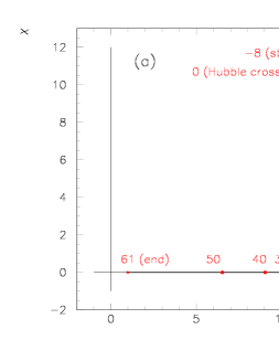
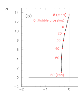
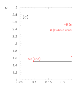
Figure 1: Examples of classical inflationary trajectories for double inflation with canonical kinetic terms (left), double inflation with non-canonical kinetic terms (center) and roulette inflation (right). The details of the models are described in Section 5.2. Subsequent tens of efolds are indicated along the curves.

There is an enormous number of examples of inflationary models. Here we restrict our analysis to just three cases described below. We will use these examples to check the analytical results of the preceding Sections and to illustrate some generic features in the evolution of adiabatic and isocurvature perturbations.

5.2.1 Double inflation with canonical kinetic terms

Double inflation (with $b=0$) is certainly the most thoroughly studied example of multi-field inflation. It employs the potential

$$V(\phi,\chi)=\frac{1}{2}m_{\phi}^{2}\phi^{2}+\frac{1}{2}m_{\chi}^{2}\chi^{2}\,.$$ (108)

In order to make definite calculations, we set $7m_{\phi}=m_{\chi}$ and we choose the initial conditions $\phi_{i}=\chi_{i}$ (later we shall also comment on the case $\phi_{i}=50\chi_{i}$), 8 efolds before the scale we consider leaves the Hubble radius, after which inflation goes on for about $\sim 60$ efolds. The classical trajectory in field space is shown in Figure 1. In our example, the trajectory is strongly bent roughly 35th efolds after the Hubble crossing. As we shall see, it is at this moment when the adiabatic perturbations are strongly fed by the isocurvature ones.

5.2.2 Double inflation with non-canonical kinetic terms

In order to concentrate just on the effects due to the non-canonical nature of the kinetic terms, we consider a very simple generalization of the previous example by taking $b(\phi)=-\phi/M_{P}$ and $m_{\phi}=m_{\chi}$ in (108). We choose the initial conditions so that $\phi_{i}=0$. Then it is almost exlusively the field $\chi$ which slides down to the minimum of the potential during inflation, but due to non-canonicality of the kinetic terms, the interaction of $\chi$ with $\phi$ drives the latter slightly away from zero. The classical trajectory in the field space is shown in Figure 1.

5.2.3 Roulette inflation

Recently, inflation in the large volume compactification scheme in the type IIB string theory model has been investigated in [14] (see also [34]). In our notation, this model can be effectively described by

$$b(\phi)=b_{0}-\frac{1}{3}\ln\left(\frac{\phi}{M_{P}}\right)$$ (109)

and

$$V(\phi,\chi)=V_{0}+V_{1}\sqrt{\psi(\phi)}e^{-2\beta_{1}\psi(\phi)}+V_{2}\psi(\phi)e^{-\beta_{1}\psi(\phi)}\cos(\beta_{2}\chi)\,,$$ (110)

where $\psi(\phi)=(\phi/M_{P})^{4/3}$ and $b_{0}$, $V_{i}$, $\beta_{i}$ are functions of the parameters of the underlying string model. A generic feature of the potential (110) is that it has an infinite number of minima arranged periodically in $\chi$ and a plateau for large values of $\phi$, admitting a large variety of inflationary trajectories, which may end at different minima even if they originate from neighboring points in the field space – hence the model has been dubbed roulette inflation. In this work, we adopt the parameter set no. 1 (in Planck units: $b_{0}=-11$; $V_{0}=9.0\times 10^{-14}$; $V_{1}=3.2\times 10^{-4}$; $V_{2}=1.1\times 10^{-5}$; and $\beta_{1}=9.4\times 10^{5}$; $\beta_{2}=2\pi/3$) from [14] and choose the particular inflationary trajectory shown in Figure 1. For this trajectory, the factor $b_{\phi}M_{P}$ is rather large, of the order $10^{3}$, but the effect of the non-canonical kinetic terms is strongly suppressed by a very small value of $\epsilon$ on the plateau of the potential. The smallness of $\epsilon$ also suppresses the energy scale of inflation and one needs a smaller number of efolds than in the models described above. For definiteness, we assumed that there are $\sim 50$ efolds between the moment that the scale of interest crosses the Hubble radius and the end of inflation.

5.3 Numerical results for the perturbations

For the three inflationary models described in Section 5.2, we performed the numerical analysis, as described in Section 5.1. Here, we discuss the outcome for the spectra and correlations in Figures 2-4. In the right panel of each Figure we plot the evolution of ${\cal P}_{\cal R}$ and ${\cal P}_{\cal S}$, normalized to the single-field result ${\cal P}_{\cal R}^{\mathrm{sf}}$ given in eq. (89), as well as the evolution of the correlation coefficient $\tilde{\cal C}$ defined in (107) and the parameter $B$, defined in (92), which is the coupling between the isocurvature and the curvature perturbations. These quantities are plotted as functions of the number of efolds $N$ after Hubble crossing. Left panels of each Figures 2-4 are basically close-ups of the right ones to the vicinity of the Hubble crossing. There, we plot the evolution of ${\cal P}_{\cal R}$, ${\cal P}_{\cal S}$ and ${\cal C}_{\cal{RS}}$, normalized to the single-field result ${\cal P}_{\cal R}^{\mathrm{sf}}$ given in eq. (89). These are shown as functions of the variable $(k/aH)^{-1}$ which allows us to compare directly the numerical results with the predictions of the eqs. (86)-(88). Note that in the leading order in the slow-roll parameters $\ln(aH/k)=N$, hence the logarithmic scale in the left panels directly corresponds to the linear scale in the right panels. In Figures 2-4, we also plot the evolution of the spectra, denoted by the superscript $(a)$, when one assumes the constant slow-roll approximation after Hubble crossing, i.e. when one uses eqs. (95), (96) and (97).

For completeness, we also discuss briefly the particular case where the generation of isocurvature modes is effectively suppressed, situation which applies to some of the models discussed in the literature for specific parameters and/or initial conditions.

5.3.1 Double inflation with canonical kinetic terms

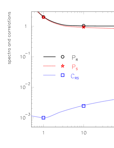
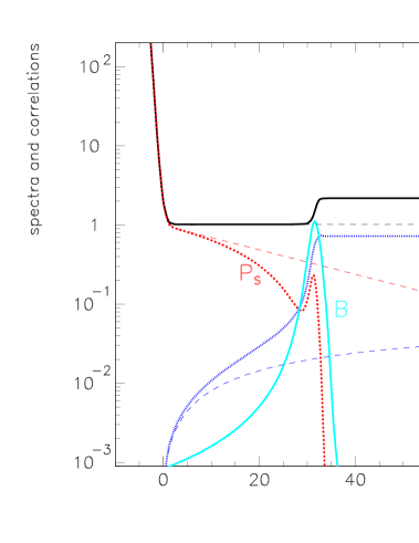
Figure 2: Predictions for the spectra and correlations of the perturbations in double inflation with canonical kinetic terms. Thick lines show the numerical results for ${\cal P}_{\cal R}$, ${\cal P}_{\cal S}$ and ${\cal C}_{\cal{RS}}$ or $\tilde{\cal C}$ normalized to the single-field result (89), respectively. Circles, stars and squares indicate the predictions of eqs. (86), (87) and (88), respectively. Thin dashed lines indicate the predictions of eqs. (95), (96) and (97), respectively. The coupling $B$ between the curvature and isocurvature perturbations is also shown.

In this example, the field $\chi$ initially dominates the energy density of the Universe and drives the first part of inflation, and only when it is almost at its minimum, inflation is further driven by $\phi$. All the slow-roll parameters are small at the Hubble crossing, which makes eqs. (86)-(88) an excellent approximation of the numerical solutions of the equations of motion. Due to the smallness of $B=-2\eta_{\sigma s}\approx 2\mathrm{d}\theta/\mathrm{d}N$ right after the Hubble crossing, the curvature perturbations become practically constant during the $\chi$-domination. At the transition to $\phi$-dominated inflation $B$ becomes large, which leads to a sizable increment in $\mathcal{P}_{\mathcal{R}}$ because of interaction with the isocurvature perturbations. During $\phi$-dominated inflation the trajectory is almost straight again, the isocurvature perturbations decay quickly and the curvature perturbations are frozen at the value acquired at the transition.

This model has the advantage that the numerical results can be directly compared to analytical ones, as the time evolution of the perturbations can be solved without assuming constancy of the slow-roll parameters [10], and we find a good agreement between two approaches.

5.3.2 Double inflation with non-canonical kinetic terms

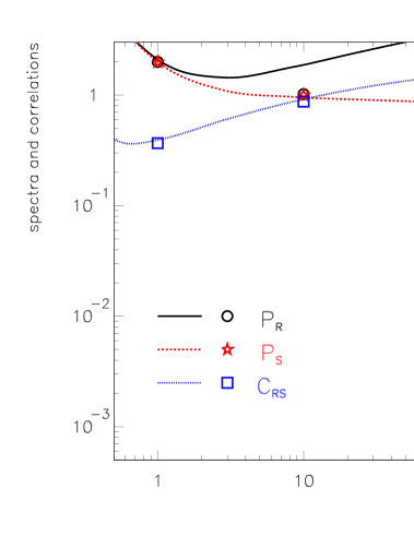
Figure 3: Predictions for the spectra and correlations of the perturbations in double inflation with non-canonical kinetic terms. Thick lines show the numerical results for ${\cal P}_{\cal R}$, ${\cal P}_{\cal S}$ and ${\cal C}_{\cal{RS}}$ or $\tilde{\cal C}$ normalized to the single-field result (89), respectively. Circles, stars and squares indicate the predictions of eqs. (86), (87) and (88), respectively. Thin dashed lines indicate the predictions of eqs. (95), (96) and (97), respectively. The coupling $B$ between the curvature and isocurvature perturbations is also shown.

In this example, the background trajectory is almost straight. However, the slow-roll parameter $\epsilon$ is around $0.1$, which makes the coupling $B$ large throughout the entire inflationary era. Figure 3 shows that eqs. (86)-(88) are a good approximation for the spectra and correlations at the Hubble crossing, $k/aH=1$, but it is no longer true at super-Hubble scales, $k/aH=0.1$ or $0.01$, because the isocurvature perturbations already start feeding the curvature ones sizably. As a result, the final curvature perturbations originate almost exclusively from the interactions with the isocurvature modes, not from the fluctuations along the inflationary trajectory, which makes the relative correlation coefficient very close to 1.

5.3.3 Roulette inflation

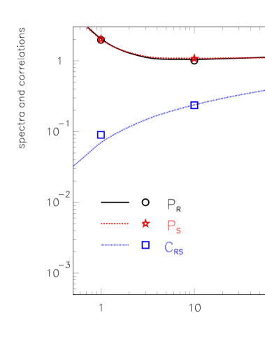
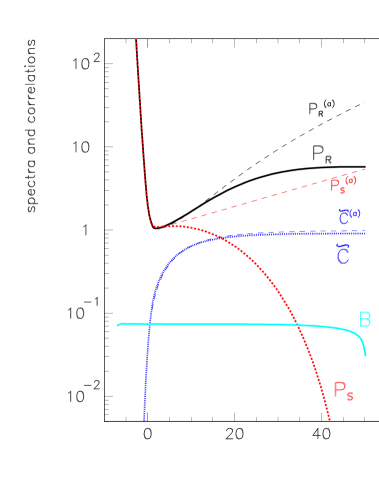
Figure 4: Predictions for the spectra and correlations of the perturbations in roulette inflation. Thick lines show the numerical results for ${\cal P}_{\cal R}$, ${\cal P}_{\cal S}$ and ${\cal C}_{\cal{RS}}$ or $\tilde{\cal C}$ normalized to the single-field result (89), respectively. Circles, stars and squares indicate the predictions of eqs. (86), (87) and (88), respectively. Thin dashed lines indicate the predictions of eqs. (95), (96) and (97), respectively. The coupling $B$ between the curvature and isocurvature perturbations is also shown.

As we already argued in Section 5.2, most of the inflationary trajectory in this example lies on the plateau of the potential (110), the slow-roll parameter $\epsilon$ is very small, which makes the direct impact of the non-canonicality negligible. The trajectory is, however, strongly curved in the field space and the interaction between the isocurvature and curvature modes is still important. Again, eqs. (86)-(88) accurately predict the spectra and correlations in the vicinity of the Hubble crossing, with deviations on super-Hubble scales resulting from the sourcing of the curvature perturbations by the isocurvature ones. Eventually, most of the curvature perturbations arise through this effect.

5.3.4 Impact of the non-canonical terms

In order to estimate the impact of the non canonical kinetic terms, one can separate each of the coefficients (36-39) into two parts: the terms that depend explicitly on the derivatives of non-canonical function $b$ and those which do not. For example, the coefficient that is directly responsible for the transfer of isocurvature modes into curvature modes, $C_{\sigma s}$ is decomposed into a ‘canonical’ component $C^{\rm(c)}_{\sigma s}$ and a ’non-canonical’ component $C^{\rm(nc)}_{\sigma s}$:

$$C_{\sigma s}=C^{\rm(c)}_{\sigma s}+C^{\rm(nc)}_{\sigma s},$$ (111)

with

$$C^{\rm(c)}_{\sigma s}=6H\frac{V_{s}}{\dot{\sigma}}+\frac{2V_{\sigma}V_{s}}{\dot{\sigma}^{2}}+2V_{\sigma s}+\frac{\dot{\sigma}V_{s}}{M_{P}^{2}H},\quad C^{\rm(nc)}_{\sigma s}=2b_{\phi}(s_{\theta}^{3}V_{\sigma}-c_{\theta}^{3}V_{s}).$$ (112)

The other coefficients can be decomposed similarly.

For the two models with non-canonical kinetic terms, we have compared in Fig. 5 the canonical and non-canonical contributions of the various coefficients. For double inflation with non-canonical kinetic terms, the non-canonical contribution in $C_{\sigma s}$ is dominant and therefore plays a crucial role in the evolution of the curvature mode. For roulette inflation, as already noticed earlier, the non-canonical contributions turn out to be negligible.

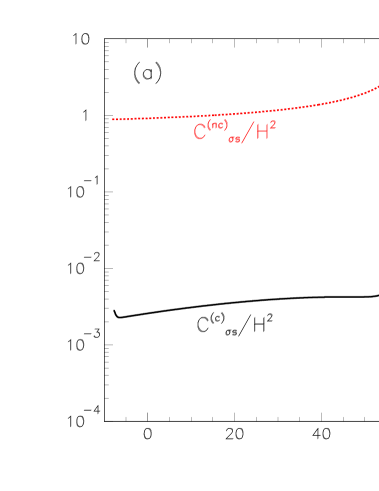
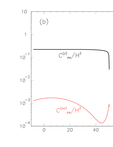
Figure 5: Evolution of the coefficients $C^{\rm(c)}_{\sigma s}$ and $C^{\rm(nc)}_{\sigma s}$ defined in (112), parametrizing the coupling between the curvature and isocurvature modes: (a) for double inflation with non-canonical kinetic terms and (b) for roulette inflation.

5.3.5 Effectively single-field cases

Figure 6: Predictions for the spectra and correlations of the perturbations in the effective single-field case. The lines show the numerical results for ${\cal P}_{\cal R}$ and ${\cal P}_{\cal S}$, circles correspond to prediction of eq. (86) and stars correspond to the analytic calculation outlined in Section 5.3.5.

Many supergravity- or string-inspired models aim at describing supersymmetry breaking and inflation in a unified framework. Often, despite the presence of many scalar fields, one can find model parameters and initial conditions such that only for one combination of the fields a potential is sufficiently flat to support inflation, e.g. in pseudo-Goldstone inflation [15], “better racetrack” scenario [16], no-scale supergravity models with moduli stabilised through D-terms [17] or in D-term uplifted supergravity of [18]. In these works, small values of the field velocity (i.e. $\epsilon\ll 1$) have been ensured by setting the initial conditions in the vicinity of the saddle point of the potential, while small curvature of the potential along one direction has been obtained by a fine-tuning of the parameters. It has been assumed that the isocurvature perturbations decay fast after the Hubble radius crossing and do not affect the curvature perturbations even though the trajectory in the field space can have sharp turns at later stages of the inflationary evolution. Consequently, the single field approximation (89) has been used in these works to account for the spectra of the curvature perturbation.

In the two-field language developed in the present paper, the situation described above corresponds to $\eta_{ss}\stackrel{{\scriptstyle>}}{{{}_{\sim}}}\mathcal{O}(1)\gg|\eta_{\sigma\sigma}|,|\eta_{\sigma s}|,\epsilon$. This justifies setting $\Theta_{*}=0$ in eqs. (76)-(78), which is equivalent to the assumption that the curvature and isocurvature modes evolve independently. While we can still apply the slow-roll expansion that led to eq. (86) for the power spectrum of the curvature perturbations, we now have to use the full result (74) to describe the spectrum of the isocurvature modes. For $\eta_{ss}\stackrel{{\scriptstyle>}}{{{}_{\sim}}}\mathcal{O}(1)$, the latter result decays very fast for $k|\tau|\to 0$ and we conclude that the isocurvature modes become irrelevant for the evolution of the curvature perturbations soon after the Hubble radius crossing.

We checked numerically that the above conclusion applies for the models described in [17], which are easily reduced to the two-field case and their inflationary trajectories are curved in the field space. For simplicity, we would like, however, to illustrate this point with the model of double inflation with standard kinetic terms, described in Section 5.2.1, for which we set the initial condition $\phi_{i}=50\chi_{i}$. Then the heavy field $\chi$ contributes negligibly to the potential energy and $\eta_{ss*}\simeq 0.4$. In Figure 6, we plot the numerically calculated spectra of the curvature and isocurvature perturbations and compare them with the analytic approximations outlined above. The decay of the isocurvature modes agrees with the solution (74), for which we show two cases: the small solid stars correspond to the constant value of $\eta_{ss}$, whereas the large empty stars show the result corresponding to adjusting the index of the Hankel function in eq. (74) to the value of $\eta_{ss}$ at a given instant, i.e. $\eta_{ss}=0.40,\,0.42,\,0.44$ for $(k/aH)^{-1}=1,\,10,\,100$, respectively. With the isocurvature modes absent, the curvature perturbations are excellently described by the single-field result, which justifies the use of the single-field approximations in the situations described above.

5.3.6 Closing discussion

The three examples presented here show that in multi-field inflationary models, a large part of the curvature perturbations can originate from interactions between the curvature and isocurvature perturbations on super-Hubble scales, not only from quantum fluctuations along the trajectory at the Hubble exit. In such cases, the single-field result (89) does not provide a correct prediction either for the normalization of the power spectrum or for its spectral index

$$n_{s}=1+\mathrm{d}\ln\mathcal{P}_{\mathcal{R}}/\mathrm{d}\ln k\,.$$ (113)

There are techniques which allow relating the spectral index of the curvature perturbations, $n_{s}$, to the spectral indices of the entropy perturbations and the curvature-entropy correlations through a set of consistency relations [19, 22, 13], but all these quantities separately depend on the super-Hubble evoulution of the perturbations. Again, we find it the most straightforward to calculate the spectral index $n_{s}$ for each model numerically. In Table 1, we compare naive estimate $n_{s}\sim 1-6\epsilon_{*}+2\eta_{\sigma\sigma*}$ and the predictions of eq. (89) for the spectral index $n_{s}$ with the numerical results of Section 5.3. In our three examples, one can see that the single-field result significantly overestimates the correct spectral index. The discrepancies that we find follow from the fact that the two types of perturbations experience the slow-roll of the background fields and the curvature of the inflationary potential in a different way. Then, if the final curvature perturbations originate mainly from the isocurvature ones, they inherit the features of the isocurvature power spectra at the Hubble crossing.

$n_{s}$	$1-6\epsilon_{*}+2\eta_{\sigma\sigma*}$	single-field result	full result
double inflation (canonical)	0.929	0.982	0.967
double inflation (non-canonical)	0.953	0.968	0.934
roulette inflation	1.017	1.019	0.932

Table 1: A comparison between the predictions for the spectral index $n_{s}$ in the three examples of inflationary models described in Section 5.2. The third column contains result derived from the single-field approximation (89); the result of full numerical calculations are shown in the fourth column.

6 Conclusion

In this paper, we have studied two-field inflation and extended several previous results on curvature and isocurvature perturbations to the case of non-standard kinetic terms.

First, we have calculated analytically the curvature and isocurvature spectra, as well as the correlation, just after Hubble crossing for two-field inflation models, including next-to-leading order corrections in the slow-roll approximation. Our results (86)-(88) generalize those of Byrnes and Wands, who assumed only standard kinetic terms. We have also given a refined analytical treatment of the spectra around Hubble crossing, which is important when the perturbations still evolve after Hubble crossing.

Second, we have studied numerically the evolution of the curvature and isocurvature perturbations after the Hubble crossing. This type of analysis is important since in multi-field inflation, in contrast with single-field inflation, the curvature perturbation spectrum after inflation is in general different from the curvature perturbation spectra at Hubble crossing because of isocurvature perturbations, as first emphasized in [6]. This well-known result applies to multi-field inflation with either standard or non-standard kinetic terms. This effect has been studied numerically for standard kinetic terms, using the decomposition into instantaneous curvature and isocurvature, in the analysis of [23]. We have done a similar analysis here for non-standard kinetic terms. In particular, we have compared the numerical evolution of the perturbations with an analytical approximation, which we denoted the constant slow-roll approximation: this approximation assumes not only that the slow-roll approximation is valid, but also that the slow-roll parameters remain almost constant during the subsequent evolution where isocurvature perturbations are significant. This approximation has been used in [21] to compute the “final” spectra in the context of non-standard kinetic terms. In most cases, this approximation is however not very realistic as we clearly show in our numerical study. We have also estimated the impact of non-standard kinetic terms on the coupled evolution of the curvature and isocurvature modes.

There has been a recent interest in constructing inflationary models in the context of string theory. These models naturally lead to scalar fields with non-standard kinetic terms, to which our analysis can apply. In this work, we have studied a very recent model, called ‘roulette” inflation, and computed quantitatively the final curvature spectrum, thus showing that the influence of isocurvature modes on super-Hubble scales turns out to be very important. Note that the authors of [14] computed the final curvature spectrum by using a “single inflaton approximation”. They stress however that isocurvature effects “could produce big effects”, which we indeed confirm in our analysis.

As a message of caution for the readers who are not familiar with the effect of isocurvature modes in multi-field inflation, we have also computed the spectral index for curvature perturbations in a few models and contrasted it with the value that one would naively obtain by using the curvature perturbation at Hubble radius like in single field inflation.

Finally, an interesting question, which goes beyond the scope of this paper, would be to investigate in which circumstances these multi-field models could produce isocurvature perturbations, after inflation and the reheating phase. These “primordial” isocurvature perturbations are today severely constrained by CMB data.

Acknowledgements We would like to thank V. Mukhanov for stimulating discussions. D.L. would like to thank the Institute of Theoretical Physics of Warsaw for their warm hospitaly and for their financial support via a “Marie Curie Host Fellowship for Transfer of Knowledge” , project MTKD-CT-2005-029466. Z.L. was partially supported by TOK project MTKD-CT-2005-029466, by the EC 6th Framework Programme MRTN-CT-2006-035863, and by the grant MEiN 1 P03D 014 26. S.P. was partially supported by TOK project MTKD-CT-2005-029466 and by the grant MEiN 1 P03B 099 29. The work of K.T. is partially supported by the US Department of Energy. K.T. would also like to acknowledge support from the Foundation for Polish Science through its programme START.

References

- [1] V. Mukhanov, “Physical foundations of cosmology,” Cambridge, UK: Univ. Pr. (2005) 421 p
- [2] L. A. Kofman and A. D. Linde, Nucl. Phys. B 282 (1987) 555.
- [3] V. F. Mukhanov and M. I. Zelnikov, Phys. Lett. B 263 (1991) 169.
- [4] N. Deruelle, C. Gundlach and D. Langlois, Phys. Rev. D 45, 3301 (1992); Phys. Rev. D 46 (1992) 5337.
- [5] D. Polarski and A. A. Starobinsky, Nucl. Phys. B 385 (1992) 623.
- [6] A. A. Starobinsky and J. Yokoyama, arXiv:gr-qc/9502002
- [7] D. Wands and J. Garcia-Bellido, Helv. Phys. Acta 69 (1996) 211 [arXiv:astro-ph/9608042].
- [8] J. Garcia-Bellido and D. Wands, Phys. Rev. D 54 (1996) 7181 [arXiv:astro-ph/9606047].
- [9] V. F. Mukhanov and P. J. Steinhardt, Phys. Lett. B 422 (1998) 52 [arXiv:astro-ph/9710038].
- [10] D. Langlois, Phys. Rev. D 59, 123512 (1999) [arXiv:astro-ph/9906080].
- [11] A. A. Starobinsky, S. Tsujikawa and J. Yokoyama, Nucl. Phys. B 610, 383 (2001) [arXiv:astro-ph/0107555].
- [12] N. Bartolo, S. Matarrese and A. Riotto, Phys. Rev. D 64 (2001) 083514 [arXiv:astro-ph/0106022].
- [13] B. van Tent, Class. Quant. Grav. 21 (2004) 349 [arXiv:astro-ph/0307048].
- [14] J. R. Bond, L. Kofman, S. Prokushkin and P. M. Vaudrevange, arXiv:hep-th/0612197.
- [15] Z. Lalak, G. G. Ross and S. Sarkar, Nucl. Phys. B 766 (2007) 1 [arXiv:hep-th/0503178].
- [16] J. J. Blanco-Pillado et al., JHEP 0609, 002 (2006) [arXiv:hep-th/0603129].
- [17] J. Ellis, Z. Lalak, S. Pokorski and K. Turzynski, JCAP 0610, 005 (2006) [arXiv:hep-th/0606133].
- [18] B. de Carlos, J. A. Casas, A. Guarino, J. M. Moreno and O. Seto, arXiv:hep-th/0702103.
- [19] C. Gordon, D. Wands, B. A. Bassett and R. Maartens, Phys. Rev. D 63, 023506 (2001) [arXiv:astro-ph/0009131].
- [20] F. Di Marco, F. Finelli and R. Brandenberger, Phys. Rev. D 67, 063512 (2003) [arXiv:astro-ph/0211276].
- [21] F. Di Marco and F. Finelli, Phys. Rev. D 71, 123502 (2005) [arXiv:astro-ph/0505198].
- [22] C. T. Byrnes and D. Wands, Phys. Rev. D 74, 043529 (2006) [arXiv:astro-ph/0605679].
- [23] S. Tsujikawa, D. Parkinson and B. A. Bassett, Phys. Rev. D 67, 083516 (2003) [arXiv:astro-ph/0210322].
- [24] K. Y. Choi, L. M. H. Hall and C. van de Bruck, JCAP 0702 (2007) 029 [arXiv:astro-ph/0701247].
- [25] H. Kodama and M. Sasaki, Prog. Theor. Phys. Suppl. 78, 1 (1984).
- [26] V. F. Mukhanov, H. A. Feldman and R. H. Brandenberger, Phys. Rept. 215, 203 (1992).
- [27] D. Langlois, “Inflation, quantum fluctuations and cosmological perturbations,” Lectures given at Cargese School of Particle Physics and Cosmology: the Interface, Cargese (2003). Published in “Cargese 2003, Particle physics and cosmology”,p 235-278. arXiv:hep-th/0405053.
- [28] D. Langlois and F. Vernizzi, JCAP 0702, 017 (2007) [arXiv:astro-ph/0610064].
- [29] D. Langlois and F. Vernizzi, Phys. Rev. Lett. 95, 091303 (2005) [arXiv:astro-ph/0503416].
- [30] D. Langlois and F. Vernizzi, Phys. Rev. D 72, 103501 (2005) [arXiv:astro-ph/0509078].
- [31] A. A. Starobinsky, JETP Lett. 42, 152 (1985) [Pis. Hz. Esp. Tor. Fizz. 42, 124 (1985)].
- [32] M. Sasaki and E. D. Stewart, Prog. Theor. Phys. 95, 71 (1996) [arXiv:astro-ph/9507001].
- [33] M. Sasaki and T. Tanaka, Prog. Theor. Phys. 99, 763 (1998) [arXiv:gr-qc/9801017].
- [34] J. P. Conlon and F. Quevedo, JHEP 0601, 146 (2006) [arXiv:hep-th/0509012].