Theory of polariton mediated Raman scattering in microcavities

Abstract

We calculate the intensity of the polariton mediated inelastic light scattering in semiconductor microcavities. We treat the exciton-photon coupling nonperturbatively and incorporate lifetime effects in both excitons and photons, and a coupling of the photons to the electron-hole continuum. Taking the matrix elements as fitting parameters, the results are in excellent agreement with measured Raman intensities due to optical phonons resonant with the upper polariton branches in II-VI microcavities with embedded CdTe quantum wells.

Planar semiconductors microcavities (MC’s) have attracted much attention in the last decade as they provide a novel means to study, enhance and control the interaction between light and matter Libro-CavityPolaritons(03) ; SemicondSciTech18-issue10(03) ; sijpcm ; Skolnick_SST98 ; Kasprzak_Nature06 ; Deng-PRL97-146401(06) ; Trigo . When the MC mode (cavity-photon) is tuned in near resonance with the embedded quantum-well (QW) exciton transitions, and the damping processes involved are weak in comparison to the photon-matter interaction, the eigenstates of the system become mixed exciton-photon states, cavity-polaritons, which are in part light and in part matter bosonic quasi-particles Libro-CavityPolaritons(03) ; SemicondSciTech18-issue10(03) ; sijpcm . Examples of interesting new physics are the recent evidence of a Bose-Einstein condensation of polaritons in CdTe MC’s Kasprzak_Nature06 ; Deng-PRL97-146401(06) , and the construction of devices which increase the interaction of sound and light, opening the possibility of realizing a coherent monochromatic source of acoustic phonons Trigo .

Raman scattering due to longitudinal optical (LO) phonons, being a coherent process is intrinsically connected with the cavity-polariton. The physics of strongly coupled photons and excitons, the polariton–phonon interaction, and the polariton–external-photon coupling are clearly displayed Fainstein_PRL97 ; Fainstein_PRB98 ; Bruchhausen_PRB03 ; Tribe_PRB97 ; Stevenson_PRB03 . In particular resonant Raman scattering (RRS) experiments, in which the wave-length of the incoming radiation is tuned in a way such that, after the emission of a LO phonon, the energy of the outgoing radiation coincides with that of the cavity polariton branches, have proven to be suited to sense the dynamics of the coupled modes, and to obtain information about the dephasing of the resonant polaritonic state Fainstein_PRL97 ; Tribe_PRB97 ; Fainstein_PRB98 ; Stevenson_PRB03 ; Bruchhausen_PRB03 . Unfortunately, due to the large remaining luminesence, RRS experiments in resonance with the lower polariton branch have not yet been achieved in intrinsic II-VI MC’s note1 . Therefore all reported experiments in these kind of MC’s, with embedded CdTe QW’s, consider the case of the scattered photons in outgoing resonance with the upper polariton branch (for two branch-systems: coupling of one exciton mode and the cavity photon) or with the middle polariton branch (for tree branch-systems: coupling of two exciton modes and the cavity photon) Fainstein_PRB98 ; Bruchhausen_PRB03 ; bru6 . The measured intensities in these two systems were analyzed on the basis of a model in which one (two) exciton states $|e\rangle$ are mixed with a photon state $|f\rangle$ with the same in-plane wave vector k, leading to a 2x2 (3x3) matrix. Essentially, the Raman intensity is proportional to

$$I\sim T_{i}T_{s}|\langle P_{i}|H^{\prime}|P_{s}\rangle|^{2},$$ (1)

where $T_{i}$ describe the probability of conversion of an incident photon $|f_{i}\rangle$ into the polariton state $|P_{i}\rangle$, $T_{s}$ has an analogous meaning for the scattered polariton $|P_{s}\rangle$ and the outgoing photon $|f_{s}\rangle$, and $H^{\prime}$ is the interaction between electrons and the LO phonons. At the conditions of resonance with the outgoing polariton, $T_{i}$ is very weakly dependent on laser energy or detuning (difference between photon and exciton energies), while $T_{s}$ is proportional to the photon strength of the scattered polariton $|\langle f_{s}|P_{s}\rangle|^{2}$. Similarly, in the simplest case of only one exciton (2x2 matrix) one expects that the matrix element entering Eq. (1) is proportional to the exciton part of the scattered polariton $|\langle P_{i}|H^{\prime}|P_{s}\rangle|^{2}\sim|\langle e_{s}|P_{s}\rangle|^{2}$. Thus if the wave function is $|P_{s}\rangle=\alpha|f_{s}\rangle+\beta|e_{s}\rangle$, one has

$$I\sim|\langle f_{s}|P_{s}\rangle|^{2}|\langle e_{s}|P_{s}\rangle|^{2}=|\alpha|^{2}|\beta|^{2}.$$ (2)

This model predicts a Raman intensity which is symmetric with detuning and is maximum at zero detuning. In other words, the intensity is maximum for detunings such that the scattered polariton is more easily coupled to the external photons, but at the same time when the polariton is more easily coupled to the optical phonons, which requires a large matter (exciton) component of the polariton. This result is in qualitative agreement with experiment Bruchhausen_PRB03 . However, for positive detuning the experimental results fall bellow the values predicted by Eq. (2) (see Fig. 1). This is ascribed to the effects of the electron-hole continuum above the exciton energy, which are not included in the model Bruchhausen_PRB03 .

For another sample in which two excitons are involved, the above analysis can be extended straightforwardly and the intensity depends on the amplitudes of a 3x3 matrix and matrix element of $H^{\prime}$ involving both excitons Bruchhausen_PRB03 . However, comparison with experiments at resonance with the middle polariton branch, shows a poorer agreement than in the previous case (Fig. 6 of Ref. Bruchhausen_PRB03, ). In addition, a loss of coherence between the scattering of both excitons with the LO phonon was assumed, which is hard to justify. Some improvement has been obtained recently when damping effects are introduced phenomenologically as imaginary parts of the photon and exciton energies, but still a complete loss of coherence resulted from the fit Bruchhausen_AIP05 ; bru6 .

In this paper we include the states of the electron-hole continuum, and the damping effects in a more rigorous way. Using some matrix elements as free parameters, we can describe accurately the Raman intensities for both samples studied in Ref. Bruchhausen_PRB03, .

In the experiments with CdTe QW’s inside II-VI MC’s, the light incides perpendicular to the $(x,y)$ plane of the QW’s and is collected in the same direction $z$. Therefore the in-plane wave vector $\mathbf{K}=0$, the polarization of the electric field should lie in the $(x,y)$ plane, and the excitons which couple with the light should have the same symmetry as the electric field (one of the two $\Gamma_{5}$ states of heavy hole excitons Jorda_PRB93 ). Thus, to lighten the notation we suppress wave vector and polarization indices. The basic ingredients of the theory are two or three strongly coupled boson modes, one for the light MC eigenmode with boson creation operator $f^{\dagger}$, another one for the $1s$ exciton ($e_{1}$) and if is necessary, the $2s$ exciton ($e_{2}$) is also included. We assume that each of these boson states mixes with a continuum of bosonic excitations which broadens its spectral density. In addition, we include the electron-hole continuum above the exciton states, described by bosonic operators $c_{\textbf{k}}^{\dagger},c_{\textbf{k}}$, where k is the difference between electron and hole momentum in the $(x,y)$ plane (the sum is $\mathbf{K}=0$ because it is conserved).

The Hamiltonian reads:

$$H = E_{f}f^{\dagger}f+\sum_{i}E_{i}e_{i}^{\dagger}e_{i}+\sum_{i}(V_{i}e_{i}^{\dagger}f+\text{H.c.})+\sum_{p}\epsilon_{p}r_{p}^{\dagger}r_{p}+\sum_{p}(V_{p}r_{p}^{\dagger}f+\text{H.c.})$$ (3)

$$+ \sum_{i\textbf{q}}\epsilon_{i\textbf{q}}d_{i\textbf{q}}^{\dagger}d_{i\textbf{q}}+\sum_{i\textbf{q}}(V_{i\textbf{q}}d_{i\textbf{q}}^{\dagger}e_{i}+\text{H.c.})+\sum_{\textbf{k}}\epsilon_{\textbf{k}}c_{\textbf{k}}^{\dagger}c_{\textbf{k}}+\sum_{\textbf{k}}(V_{\textbf{k}}c_{\textbf{k}}^{\dagger}f+\text{H.c.}).$$

The first three terms describe the strong coupling between the MC photon and the exciton(s) already included in previous approaches Bruchhausen_PRB03 ; Bruchhausen_AIP05 . The fourth and fifth terms describe a continuum of radiative modes and its coupling to the MC light eigenmode. Their main effect is to broaden the spectral density of the latter even in the absence of light-matter interaction. The following two terms have a similar effect for the exciton mode(s). The detailed structure of the states described by the $d_{i\textbf{q}}^{\dagger}$ operators is not important in what follows. They might describe combined excitations due to scattering with acoustical phonons. The last two terms correspond to the energy of the electron hole excitations and their coupling to the MC light mode.

In Eq. (3) we are making the usual approximation of neglecting the internal fermionic structure of the excitons and electron-hole operators and taking them as free bosons. This is an excellent approximation for the conditions of the experiment. We also neglect terms which do not conserve the number of bosons. Their effect is small for the energies of interest Jorda_PRB94 . These approximations allow us formally to diagonalize the Hamiltonian by a Bogoliubov transformation. The diagonalized Hamiltonian has the form $H=\sum_{\nu}E_{\nu}p_{\nu}^{\dagger}p_{\nu}$, where the boson operators $p_{\nu}^{\dagger}$ correspond to generalized polariton operators and are linear combinations of all creation operators entering Eq. (3). Denoting the latter for brevity as $b_{j}^{\dagger}$, then $p_{\nu}^{\dagger}=\sum_{j}A_{\nu j}b_{j}^{\dagger}$. In practice, instead of calculating the $E_{\nu}$ and $A_{\nu j}$, it is more convenient to work with retarded Green’s functions $G_{jl}(\omega)=\langle\langle b_{j};b_{l}^{\dagger}\rangle\rangle_{\omega}$ and their equations of motion

$$\omega\langle\langle b_{j};b_{l}^{\dagger}\rangle\rangle_{\omega}=\delta_{jl}+\langle\langle[b_{j},H];b_{l}^{\dagger}\rangle\rangle_{\omega}.$$ (4)

As we show below, the RRS intensity can be expressed in terms of spectral densities derived from these Green’s functions, which in turn can be calculated using Eq. (4).

Using Fermi’s golden rule, the probability per unit time for a transition from a polariton state $|i\rangle=p_{\nu^{\prime}}^{\dagger}|0\rangle$ to states $|s\rangle=p_{\nu}^{\dagger}a^{\dagger}|0\rangle$, where $a^{\dagger}$ creates a LO phonon is

$$W=\frac{2\pi}{\hbar}|\langle i|H^{\prime}|s\rangle|^{2}\rho(\omega),\;\;\text{where}\;\;\rho(\omega)=\sum_{\nu}\delta(\omega-E_{\nu})=-\frac{1}{\pi}\text{Im}G_{\nu\nu}(\omega+i0^{+})$$ (5)

is the density of final states. As argued above, we neglect the dependence of $T_{i}$ on frequency and take $T_{s}=|A_{\nu f}|^{2}$, the weight of photons in the scattered eigenstates. In addition, $H^{\prime}$ should be proportional to the matter (exciton) part of the scattered polariton states. Then, the Raman intensity is proportional to:

$$WT_{s}\propto I=|A_{\nu e1}+\alpha A_{\nu e2}|^{2}|A_{\nu f}|^{2}\rho(\omega).$$ (6)

Here we are neglecting the contribution of the electron-hole continuum to $H^{\prime}$, and $\alpha$ is the ratio of matrix elements of the exciton-LO phonon interaction between $2s$ and $1s$ excitons. If the $2s$ excitons are unimportant, $\alpha=0$.

Using Eqs. (4) it can be shown that

$$\rho_{jl}(\omega) = -\frac{1}{2\pi}[G_{jl}(\omega+i0^{+})-G_{jl}(\omega-i0^{-})]=A_{\nu j}\bar{A}_{\nu l}\rho(\omega).$$ (7)

From here and $\sum_{j}|A_{\nu j}|^{2}=1$, it follows that $\rho(\omega)=\sum_{j}\rho_{jj}(\omega)$. Replacing in Eq. (6) we obtain:

$$I(\omega)=\frac{\rho_{ff}[\rho_{e1,e1}+|\alpha|^{2}\rho_{e2,e2}+2\text{Re}(\alpha\rho_{e2,e1})]}{\sum_{j}\rho_{jj}(\omega)}.$$ (8)

In practice, when $\omega$ is chosen such that the resonance condition for the outgoing polariton is fulfilled, we can neglect the contribution of the continuum states in the denominator of Eq. (8). In particular, if the contribution of the $2s$ exciton can be neglected (as in sample A of Ref. Bruchhausen_PRB03, )

$$I(\omega)=\frac{\rho_{ff}(\omega)\rho_{e1,e1}(\omega)}{\rho_{ff}(\omega)+\rho_{e1,e1}(\omega)}.$$ (9)

The Green’s functions are calculated from the equations of motion (4). In the final expressions, the continuum states enter through the following sums:

$$S_{f}(\omega) = \sum_{p}\frac{|V_{p}|^{2}}{\omega+i0^{+}-\epsilon_{p}},\;\;S_{i}(\omega)=\sum_{\textbf{q}}\frac{|V_{i\textbf{q}}|^{2}}{\omega+i0^{+}-\epsilon_{i\textbf{q}}},\;\;S_{f}^{\prime}(\omega)=\sum_{\textbf{k}}\frac{|V_{\textbf{k}}|^{2}}{\omega+i0^{+}-\epsilon_{\textbf{k}}}$$ (10)

For the first two we assume that the results are imaginary constants that we take as parameters:

$$S_{f}(\omega)=-i\delta_{f},\;\;\;\;\ S_{j}(\omega)=-i\delta_{j}$$ (11)

This is the result expected for constant density of states and matrix elements. Our results seem to indicate that this assumption is valid for the upper and middle polariton branches. For the lower branch at small k it has been shown that the line width due to the interaction of polaritons with acoustic phonons depends on detuning $E_{f}-E_{1}$ and $k_{\parallel}$, being smaller for small wave vector Savona_PSS97 ; Cassabois_PRB00 .

The electron-hole continuum begins at the energy of the gap and corresponds to vertical transitions in which the light promotes a valence electron with 2D wave vector k to the conduction band with the same wave vector. In the effective-mass approximation, the energy is quadratic with k and this leads to a constant density of states beginning at the gap. The matrix element $V_{\textbf{k}}$ is proportional to $M_{\textbf{k}}=\langle\textbf{k}_{v}|p_{E}|\textbf{k}_{c}\rangle$, where $p_{E}$ is the momentum operator in the direction of the electric field, and $|\textbf{k}_{v}\rangle$, $|\textbf{k}_{c}\rangle$ are the wave functions for valence and conduction electrons with wave vector k. Taking these wave functions as plane waves, one has $M_{\textbf{k}}\sim k_{E}$, the wave vector in the direction of the electric field. Then $|V_{\textbf{k}}|^{2}\sim k_{E}^{2}$. Adding the contributions of all directions of k one has $|V_{\textbf{k}}|^{2}\sim|\textbf{k}|^{2}\sim\epsilon_{\textbf{k}}$ (linear with energy for small energy). This leads to

$$S_{f}^{\prime}=R(\omega)-iA(\omega-B)\Theta(\omega-B),$$ (12)

where $B$ is the bottom of the electron-hole continuum (the energy of the semiconductor gap) and $A$ is a dimensionless parameter that controls the magnitude of the interaction. The real part $R(\omega)$ can be absorbed in a renormalization of the photon energy and is unimportant in what follows. The imaginary part is a correction to the photon width for energies above the bottom of the continuum.

Using the theory outlined above, we calculated the intensity of RRS corresponding to the samples A and B measured in Refs. Bruchhausen_PRB03, ; bru6, and compared them with the experimental results.

Sample A corresponds to the simplest case. Two polariton branches are seen and therefore only the $1s$ exciton plays a significant role. The binding energy of this exciton $B-E_{1}$ is not well known. The Rabi splitting $2V_{1}=19$ meV. The width of the Raman scan as a function of frequency for zero detuning is of the order of $w=0.1$ meV (see Fig. 3 of Ref. Bruchhausen_PRB03, ). This implies the relation $2w^{2}=\delta_{f}^{2}+\delta_{1}^{2}$ in our theory. In any case the results are weakly sensitive to $w$. Therefore, we have three free parameters in our theory in addition to a multiplicative constant: $B-E_{1}$, the ratio of widths $\delta_{f}/\delta_{1}$ and the slope $A$.

Figure 1: Raman intensity as a function of detuning for sample A. Solid squares: experimental results Bruchhausen_PRB03 . Solid line: theory (Eq. 9) for $B-E_{1}=14$ meV, $\delta_{f}=\delta_{1}=0.1$ meV, and $A=0.031$. Dashed line: result for a 2x2 matrix (Eq. 2).

The comparison between the experimental and the theoretical intensities is shown in Fig. 1 for a set of parameters that lead to a close agreement with experiment. The condition of resonance is established choosing the energy $\omega$ for which the intensity given by Eq. (9) has its second relative maximum (corresponding to the upper polariton branch). The dashed line corresponds to the case in which only the first three terms (with $i=1$) in the Hamiltonian, Eq. (3) are included. In this case, the intensity is given in terms of the solution of a 2x2 matrix [Eq. (2)] and was used in Ref. Bruchhausen_PRB03, to interpret the data. This simple expression gives a Raman intensity which is an even function of detuning. When the full model is considered, the Raman intensity falls more rapidly for large detuning $E_{f}-E_{1}$ as a consequence of the hybridization of the photon with the electron-hole continuum. When the energy of the polariton increases beyond $B$ entering the electron-hole continuum (corresponding to the kink in Fig. 1), the Raman peak broadens and loses intensity. The kink can be smoothed if the effect of the infinite excitonic levels below the continuum is included in the model (leading to an $S_{f}^{\prime}$ with continuous first derivative), but this is beyond the scope of this work. If the ratio $\delta_{f}/\delta_{1}$ is enlarged, the Raman intensity increases for negative detuning with respect to its value for positive detuning.

In the experiments with sample B three polariton branches are observed bru6 and the $2s$ exciton plays a role. Experimentally, it is known that the binding energy for the two excitons are $B-E_{1}=$17 meV and $B-E_{2}=$2 meV. From the observed Rabi splitting one has $2V_{1}=13$ meV, $2V_{2}=2.5$ meV. In comparison with the previous case, we have the additional parameter $\alpha$ (the ratio of exciton-LO phonon matrix elements). In addition, to be able to describe well the intensity for low energies of the middle polariton (left part of the curve shown in Fig. 2), we need to assume a small linear dependence of $E_{1}$ with the position of the incident laser spot in the sample. This dependence is also inferred form the observed luminescence spectrum bru6 . In our model, this corresponds to a dependence of $E_{1}$ with $E_{f}$:

$$E_{1}=E_{1}^{0}+z(E_{f}-E_{1}^{0})$$ (13)

In Fig. 2 we show the intensity at the second maximum of $I(\omega)$ (corresponding to the middle polariton branch) as a function of the energy of this maximum. We also show in the figure experimental results taken at lower laser excitation and a slightly higher temperature (4.5 K) than those reported in Ref. Bruchhausen_PRB03, .

The slope which better describes the data is $z=0.14$. This value is close to $z=0.155$ which was obtained from a fit of the maxima of luminescence spectrum of the lower and middle polaritons. We have taken the same value for $A$ as in Fig. 1. The agreement between theory and experiment is remarkable. As for sample A, the values of $\delta_{i}$ that result from the fit are reasonable in comparison with calculated values Savona_PSS97 .

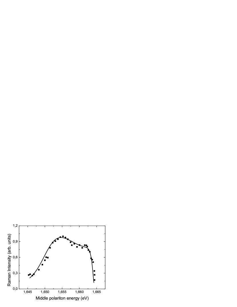
Figure 2: Raman intensity as a function of the middle polariton energy. Solid squares: experimental results bru6 . Solid line: theory for $\delta_{f}=0.2$ meV, $\delta_{1}=0.1$ meV, $\delta_{2}=0.12$ meV, $\alpha=-0.45$ and $z=0.14$. $A$ is the same as in Fig. 1 .

In summary, we have proposed a theory to calculate Raman intensity for excitation of longitudinal optical phonons in microcavities, in which different matrix elements are incorporated as parameters of the model. The most important advance in comparison with previous simplified theories Bruchhausen_PRB03 ; Bruchhausen_AIP05 is the inclusion of the strong coupling of the electron-hole continuum with the microcavity photon. Inclusion of this coupling is essential when the energy of the polariton is near the bottom of the conduction band (at the right of Fig. 1). We also have included the effects of damping of excitons and photons, coupling them with a continuum of bosonic excitations. Simpler approaches have included the spectral widths $\delta_{f}$ and $\delta_{i}$ of photons and excitons as imaginary parts of the respective energies, leading to non-hermitian matrices.

Taking some of the parameters of the model as free ($\delta_{f}/\delta_{i}$, $B-E_{1}$ and $A$ for sample A, $\delta_{f}$, $\delta_{i}$, $z$ and $\alpha$ for sample B), we obtain excellent fits of the observed Raman intensities. The resulting values of the parameters agree with previous estimates, if they are available. We are not aware of previous estimates for $A$ and $\alpha$. As an important improvement to previous approaches Bruchhausen_PRB03 ; Bruchhausen_AIP05 for the case of sample B, we do not have to assume a partial loss of coherence between $1s$ and $2s$ excitons in their scattering with the LO phonon.

Further progress in the understanding of the interaction of excitons with light and phonons requires microscopic calculations of the parameters $\delta_{f},\delta_{i},A$ and $\alpha$, and the effects of the temperature on them. However, taking into account the difficulties in calculating these parameters accurately, the present results are encouraging and suggest that the main physical ingredients are included in our model.

We thank A. Fainstein for useful discussions. This work was supported by PIP 5254 of CONICET and PICT 03-13829 of ANPCyT.

References

- (1) Kavokin A and Malpuech G 2003 Cavity Polaritons (Elsevier, Amsterdam)
- (2) Special issue on microcavities 2003 Semicond. Sci. Technol. 18 10 S279-S434
- (3) Special issue on Photon-mediated phenomena in semiconductor nanostructures J. Phys. Condens. Matter 18 35 S3549-S3768
- (4) Skolnick M S, Fisher T and Whittaker D M 1998 Semicond. Sci. Technol 13 645
- (5) Kasprzak J, Richard M, Kundermann M, Baas A, Jeambrun P, Keeling J M J, Marchetti F M, Szymanska M H, André R, Staehli J L, Savona V, Littlewood P B, Deveaud B and Le Si Dang 2006 Nature 443 409
- (6) Deng H, Press D, Götzinger S, Solomon G S, Hey R, Ploog K H and Yamamoto Y 2006 Phys. Rev. Lett. 97 146402
- (7) Trigo M, Bruchhausen A, Fainstein A, Jusserand B and Thierry-Mieg V 2002 Phys. Rev. Lett. 89 227402
- (8) Fainstein A, Jusserand B and Thierry-Mieg V 1997 Phys. Rev. Lett. 78 1576
- (9) Fainstein A, Jusserand B and André R 1998 Phys. Rev. B 57 R9439
- (10) Bruchhausen A, Fainstein A, Jusserand B and André R 2003 Phys. Rev. B 68 205326
- (11) Tribe W R, Baxter D, Skolnick M S, Mowbray D J, Fisher T A and Roberts J S 1997 Phys. Rev. B 56 12 429
- (12) Stevenson R M, Astratov V N, Skolnick M S, Roberts J S and Hill G 2003 Phys. Rev. B 67 081301(R)
- (13) RRS experiments in resonance with the lower polariton branch have only been reported in III-VI samples with doped Bragg reflectors (see refs. Tribe_PRB97 and Stevenson_PRB03 for details).
- (14) Fainstein A and Jusserand B 2006 in Light Scattering in Solids vol. 9 Cardona M and Merlin R editors (Springer, Berlin)
- (15) Bruchhausen A, Fainstein A and Jusserand B 2005 Physics of semiconductors CP772 p.1117 Menéndez J and Van de Walle C G editors (American Institute of Physics)
- (16) Jorda S, Rössler U and Broido D 1993 Phys. Rev. B 48 1669
- (17) Jorda S 1994 Phys. Rev. B 50 2283
- (18) Savona V and Piermarocchi C 1997 Phys. Status Solidi A 164 45
- (19) Cassabois G, Triques A L C, Bogani F, Delalande C, Roussignol Ph and Piermarocchi C 2000 Phys. Rev. B 61 1696