Thermal entanglement of qubit pairs on the Shastry-Sutherland lattice

Abstract

We show that temperature and magnetic field properties of the entanglement between spins on the two-dimensional Shastry-Sutherland lattice can be qualitatively described by analytical results for a qubit tetramer. Exact diagonalization of clusters with up to 20 sites reveals that the regime of fully entangled neighboring pairs coincides with the regime of finite spin gap in the spectrum. Additionally, the results for the regime of vanishing spin gap are discussed and related to the Heisenberg limit of the model.

I Introduction

In any physical system with subsystems in interaction, individual parts of the system are to some extent entangled, even if they are far apart, as realized already at the beginning of modern quantum mechanics sixty years ago. Today it has become appreciated that the ability to establish entanglement between quantum particles in a controlled manner is a crucial ingredient of any quantum information processing systemnielsen01 . On the other hand, it turned out that the analysis of appropriately quantified entanglement between parts of the system can also be a very useful tool in the study of many body phenomena, as is, e.g., the behavior of correlated systems in the vicinity of crossovers between various regimes or even points of quantum phase transitionosterloh02 .

Quantum entanglement of two distinguishable particles in a pure state can be quantified through von Neuman entropy bennett96 ; hill97 ; vedral97 . Entanglement between two spin-${1\over 2}$ particles – qubit pair – can be considered a physical resource, an essential ingredient of algorithms suitable for quantum computation. For a pair of subsystems A and B, each occupied by a single electron, an appropriate entanglement measure is the entanglement of formation, which can be quantified from the Wootters formulawootters98 . In general, electron-qubits have the potential for even richer variety of entanglement measure choices due to both their charge and spin degrees of freedom. When entanglement is quantified in systems of indistinguishable particles, the measure must account for the effect of exchange and it must adequately deal with multiple occupancy states schliemann01 ; ghirardi04 ; eckert02 ; gittings02 ; zanardi02 ; vedral03 . A typical example is the analysis of entanglement in lattice fermion models (the Hubbard model, e.g.) where double occupancy plays an essential rolezanardi02 .

In realistic hardware designed for quantum information processing, several criteria for qubits must be fulfilledcriteria : the existence of multiple identifiable qubits, the ability to initialize and manipulate qubits, small decoherence, and the ability to measure qubits, i.e., to determine the outcome of computation. It seems that among several proposals for experimental realizations of such quantum information processing systems the criteria for scalable qubits can be met in solid state structures consisting of coupled quantum dotsdivincenzo05 ; coish06 . Due to the ability to precisely control the number of electrons in such structures elzerman03 , the entanglement has become experimentally accessible quantity. In particular, recent experiments on semiconductor double quantum dot devices have shown the evidence of spin entangled states in GaAs based heterostuctureschen04 and it was shown that vertical-lateral double quantum dots may be useful for achieving two-electron spin entanglementhatano05 . It was also demonstrated recently that in double quantum dot systems coherent qubit manipulation and projective readout is possible petta05 .

Qubit pairs to be used for quantum information processing must be to a high degree isolated from their environment, otherwise small decoherence requirement from the DiVincenzo’s checklist can not be fulfilled. The entanglement, e.g., between two antiferromagnetically coupled spins in contact with thermal bath, is decreased at elevated temperatures and external magnetic fieldnielsen00 ; arnesen01 ; wang01 , and will inevitably vanish at some finite temperaturefine05 . Entanglement of a pair of electrons that are confined in a double quantum dot is collapsed due to the Kondo effect at low temperatures and for a very weak tunneling to the leads. At temperatures below the Kondo temperature a spin-singlet state is formed between a confined electron and conduction electrons in the leadsrmzb06 . For other open systems there are many possible sources of decoherence or phase-breaking, for example coupling to phonon degrees of freedom yu02 .

The main purpose of the present paper is to analyze the robustness of the entanglement of spin qubit pairs in a planar lattice of spins (qubits) with respect to frustration in magnetic couplings, elevated temperatures as well as due to increasing external magnetic field. The paper is organized as follows. Sec. II introduces the model for two coupled qubit pairs – qubit tetramer – and presents exact results for temperature and magnetic field dependence of the entanglement between nearest and next-nearest-neighboring spins in a tetrahedron topology. In Sec. III the model is extended to infinite lattice of qubit pairs described by the Shastry-Sutherland model shastry81 . This model is convenient firstly, because of the existence of stable spin-singlet pairs in the ground state in the limit of weak coupling between the qubit pairs, and secondly, due to a relatively good understanding of the physics of the model in the thermodynamic limit. Entanglement properties of the Shastry-Sutherland model were so far not considered quantitatively. Neverteless, several results concerning the role of entanglement at a phase transition in other low-dimensional spin lattice systems osterloh02 ; syljuasen03 ; amico04 ; osborne02 ; roscilde04 ; roscilde05 ; larsson05 , as well as in fermionic systemsgu04 ; deng05 ; legeza06 have been reported recently. Near a quantum phase transition in some cases entanglement even proves to be more efficient precursor of the transition compared to standard spin-spin correlations verstraete04 ; legeza06 . In Sec. IV we discuss entanglement between nearest neighbors in the Heisenberg model, representing a limiting case of the Shastry-Sutherland model. Results are summarized in Sec. V and some technical details are given in Appendix A.

II Thermal entanglement of a qubit tetramer in magnetic field

Consider first a double quantum dot composed of two adjacent quantum dots weakly coupled via a controllable electron-hopping integral. By adjusting a global back-gate voltage, precisely two electrons can be confined to the dots. The inter-dot tunneling matrix element $t$ determines the effective antiferromagnetic (AFM) superexchange interaction $J\sim 4t^{2}/U$, where $U$ is the scale of Coulomb interaction between two electrons confined on the same dot. There are several possible configurations of coupling between such double quantum dots. One of the simplest specific designs is shown schematically in Fig. 1(a): four qubits at vertices of a tetrahedron. In addition to the coupling A-B, by appropriate arrangements of gate electrodes the tunneling between A-C and A-D can as well be switched on.

Figure 1: (Color online) (a) Two coupled qubit pairs (dimers) in tetrahedral topology. (b) Shastry-Sutherland lattice as realized, e.g., in the SrCu₂(BO₃)₂ compound.

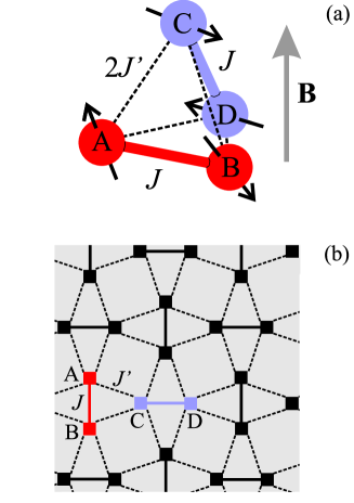
We consider here the case where $J/U\ll 1$, thus double occupancy of individual dot is negligible and appropriate Hilbert space is spanned by two dimers (qubit pairs): spins at sites A-B and C-D are coupled by effective AFM Heisenberg magnetic exchange $J$ and at sites A-C, B-C, A-D, B-D by $J^{\prime}$. The corresponding hamiltonian of such a pair of dimers is given as

$$H_{4} = J({\textbf{S}}_{\textrm{A}}\cdot{\textbf{S}}_{\textrm{B}}+{\textbf{S}}_{\textrm{C}}\cdot{\textbf{S}}_{\textrm{D}})+$$

$$+ 2J^{\prime}({\textbf{S}}_{\textrm{A}}\cdot{\textbf{S}}_{\textrm{C}}+{\textbf{S}}_{\textrm{B}}\cdot{\textbf{S}}_{\textrm{C}}+{\textbf{S}}_{\textrm{A}}\cdot{\textbf{S}}_{\textrm{D}}+{\textbf{S}}_{\textrm{B}}\cdot{\textbf{S}}_{\textrm{D}})-$$

$$- B(S^{z}_{\textrm{A}}+S^{z}_{\textrm{B}}+S^{z}_{\textrm{C}}+S^{z}_{\textrm{D}}),$$

where $\textbf{S}_{i}={1\over 2}{\bf\sigma}_{i}$ is spin operator corresponding to the site $i$ and $B$ is external homogeneous magnetic field in the direction of the $z$-axis. Factor 2 in Eq. (II) is introduced for convenience – such a parameterization represents the simplest case of finite Shastry-Sutherland lattice with periodic boundary conditions studied in Sec. III.

Figure 2: (Color online) (a) Zero-temperature concurrence $C_{\mathrm{A}\mathrm{B}}$ as a function of $J^{\prime}/J$ and $B/J$. Different regimes are characterized by particular ground state functions $|\phi_{n}\rangle$ defined in Appendix A. (b) $T/J=0.1$ results for $C_{\mathrm{A}\mathrm{B}}$. (c) Next nearest concurrence $C_{\mathrm{A}\mathrm{C}}$ for $T=0$, and (d) for $T/J=0.1$. Dashed lines separate $C_{\mathrm{A}\mathrm{B}(\mathrm{C})}>0$ from $C_{\mathrm{A}\mathrm{B}(\mathrm{C})}=0$.

II.1 Concurrence

We focus here on the entanglement properties of two coupled qubit dimers. The entanglement of a pair of spin qubits A and B may be defined through concurrencebennett96 , $C=2|\alpha_{\uparrow\!\uparrow}\alpha_{\downarrow\!\downarrow}-\alpha_{\uparrow\!\downarrow}\alpha_{\downarrow\!\uparrow}|$, if the system is in a pure state $|\Psi_{\mathrm{AB}}\rangle=\sum_{ss^{\prime}}\alpha_{ss^{\prime}}|s\rangle_{\!\mathrm{A}}|s^{\prime}\rangle_{\!\mathrm{B}}$, where $|s\rangle_{i}$ corresponds to the basis $|\!\uparrow\,\rangle_{i}$, $|\!\downarrow\,\rangle_{i}$. Concurrence varies from $C=0$ for an unentangled state (for example $|\!\uparrow\,\rangle_{\mathrm{A}}|\!\uparrow\,\rangle_{\mathrm{B}}$) to $C=1$ for completely entangled Bell statesbennett96 ${1\over\sqrt{2}}(|\!\uparrow\,\rangle_{\mathrm{A}}|\!\uparrow\,\rangle_{\mathrm{B}}\pm|\!\downarrow\,\rangle_{\mathrm{A}}|\!\downarrow\,\rangle_{\mathrm{B}})$ or ${1\over\sqrt{2}}(|\!\uparrow\,\rangle_{\mathrm{A}}|\!\downarrow\,\rangle_{\mathrm{B}}\pm|\!\downarrow\,\rangle_{\mathrm{A}}|\!\uparrow\,\rangle_{\mathrm{B}})$.

For finite inter-pair coupling $J^{\prime}\neq 0$ or at elevated temperatures the A-B pair can not be described by a pure state. In the case of mixed states describing the subsystem A-B the concurrence may be calculated from the reduced density matrix $\rho_{\textrm{A}\textrm{B}}$ given in the standard basis $|s\rangle_{i}|s^{\prime}\rangle_{j}$wootters98 . Concurrence can be further expressed in terms of spin-spin correlation functions osterloh02 ; syljuasen03 , where for systems that are axially symmetric in the spin space the concurrence may conveniently be given in a simple closed formramsak06 , which for the thermal equilibrium case simplifies further,

$$C_{\mathrm{A}\mathrm{B}}=2\textrm{max}(0,|\langle S_{\mathrm{A}}^{+}S_{\mathrm{B}}^{-}\rangle|-\sqrt{\langle P_{\mathrm{A}}^{\uparrow}P_{\mathrm{B}}^{\uparrow}\rangle\langle P_{\mathrm{A}}^{\downarrow}P_{\mathrm{B}}^{\downarrow}\rangle}).$$ (2)

Here $S_{i}^{+}=(S_{i}^{-})^{\dagger}=S_{i}^{x}+\imath S_{i}^{y}$ is the spin raising operator for dot $i$ and $P_{i}^{\uparrow}={1\over 2}(1+2S_{i}^{z})$, $P_{i}^{\downarrow}={1\over 2}(1-2S_{i}^{z})$ are the projection operators onto the state $|\!\uparrow\,\rangle_{i}$ or $|\!\downarrow\,\rangle_{i}$, respectively. We consider the concurrence at fixed temperature, therefore the expectation values in the concurrence formula Eq. (2) are evaluated as

$$\langle{\cal O}\rangle={1\over Z}\sum_{n}\langle n|{\cal O}|n\rangle e^{-\beta E_{n}},$$ (3)

where $Z=\sum_{n}e^{-\beta E_{n}}$ is the partition function, $\beta=1/T$, and $\{|n\rangle\}$ is a complete set of states of the system. Note that due to the equilibrium and symmetries of the system, several spin-spin correlation functions vanish, $\langle S_{\mathrm{A}}^{+}S_{\mathrm{B}}^{+}\rangle=0$, for example.

In vanishing magnetic field, where the SU(2) symmetry is restored, the concurrence formula Eq. (2) simplifies further and is completely determined by only onewerner89 spin invariant $\langle\textrm{\bf S}_{\mathrm{A}}\cdot\textrm{\bf S}_{\mathrm{B}}\rangle$,

$$C_{\mathrm{A}\mathrm{B}}=\textrm{max}(0,-2\langle\textrm{\bf S}_{\mathrm{A}}\cdot\textrm{\bf S}_{\mathrm{B}}\rangle-\frac{1}{2}).$$ (4)

The concurrence may be expected to be significant whenever enhanced spin-spin correlations indicate A-B singlet formation.

II.2 Analytical results

There are several known results related to the model Eq. (II). In the special case of $J^{\prime}=0$, for example, the tetramer consists of two decoupled spin dimers with concurrence $C_{\mathrm{A}\mathrm{B}}$ (or the corresponding thermal entanglement) as derived in Refs. nielsen00, ; arnesen01, . Entanglement of a qubit pair described by the related XXZ Heisenberg model with Dzyaloshinskii-Moriya anisotropic interaction can be also obtained analyticallywang01 . Hamiltonian $H_{4}$ with additional four-spin exchange interaction but in the absence of magnetic field was considered recently in the various limiting casesbose05 .

Tetramer model Eq. (II) considered here is exactly solvable and in Appendix A we present the corresponding eigenvectors and eigenenergies. The concurrence $C_{\mathrm{A}\mathrm{B}}$ is for this case determined from Eq. (2) with

$$\langle S_{\rm A}^{+}S_{\rm B}^{-}\rangle = \frac{1}{Z}\Big{[}\!\!-e^{3j/2}/2-e^{j/2}\left(e^{b}+e^{-b}\right)/2$$ (5)

$$+ e^{-j/2+4j^{\prime}}/6+e^{-j/2+2j^{\prime}}\left(e^{b}+e^{-b}\right)/4$$

$$+ e^{-j/2-2j^{\prime}}\left(e^{b}/4+1/3+e^{-b}/4\right)\!\!\Big{]},$$

where $j=\beta J$, $j^{\prime}=\beta J^{\prime}$, $b=\beta B$, and with

$$\langle P_{\rm A}^{\uparrow\downarrow}P_{\rm B}^{\uparrow\downarrow}\rangle = \frac{1}{Z}\Big{[}e^{j/2}\left(e^{\pm b}\right)+e^{-j/2+4j^{\prime}}/3$$ (6)

$$+ e^{-j/2+2j^{\prime}}\left(1+e^{\pm b}\right)/2$$

$$+ e^{-j/2-2j^{\prime}}\left(1/6+e^{\pm b}/2+e^{\pm 2b}\right)\!\!\Big{]}.$$

Here

$$Z = e^{3j/2}+2e^{j/2}\left(e^{b}+1+e^{-b}\right)$$ (7)

$$+ e^{-j/2+4j^{\prime}}+e^{-j/2+2j^{\prime}}\left(e^{b}+1+e^{-b}\right)$$

$$+ e^{-j/2-2j^{\prime}}\left(e^{2b}+e^{b}+1+e^{-b}+e^{-2b}\right)$$

is the partition function.

Figure 3: (Color online) (a) Temperature and magnetic field dependence of $C_{\mathrm{A}\mathrm{B}}$ for $J^{\prime}/J=0.4$ and (b) $J^{\prime}=J$. Dashed lines separate $C_{\mathrm{A}\mathrm{B}}>0$ from $C_{\mathrm{A}\mathrm{B}}=0$.

Alternatively, one can define and analyze also the entanglement between spins at sites A and C and the corresponding concurrence $C_{\mathrm{A}\mathrm{C}}$ can be expressed from Eq. (2) by applying additional correlators with replaced B$\to$C,

$$\langle S_{\rm A}^{+}S_{\rm C}^{-}\rangle = \frac{1}{Z}\Big{[}\!\!-e^{-j/2+4j^{\prime}}/3$$ (8)

$$- e^{-j/2+2j^{\prime}}\left(e^{b}+e^{-b}\right)/4$$

$$+ e^{-j/2-2j^{\prime}}\left(e^{b}/4+1/3+e^{-b}/4\right)\!\!\Big{]},$$

and

$$\langle P_{\rm A}^{\uparrow\downarrow}P_{\rm C}^{\uparrow\downarrow}\rangle = \frac{1}{Z}\Big{[}e^{3j/2}/4+e^{j/2}\left(1/2+e^{\pm b}\right)$$ (9)

$$+ e^{-j/2+4j^{\prime}}/12+e^{-j/2+2j^{\prime}}e^{\pm b}/2$$

$$+ e^{-j/2-2j^{\prime}}\left(1/6+e^{\pm b}/2+e^{\pm 2b}\right)\!\!\Big{]}.$$

The line $2J^{\prime}=J$ represents a particularly interesting special case where two dimers are coupled symmetrically forming a regular tetrahedron. An important property of this system is the (geometrical) frustration of, e.g., qubits C-A-B. Such a frustration is the driving force of the quantum phase transition found in the Shastry-Sutherland model and is the reason for similarity of the results for two coupled dimers and a large planar lattice studied in the next Section.

II.3 Examples

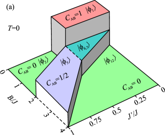
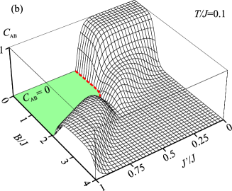
In the low temperature limit the concurrence is determined by the ground state properties while transitions between various regimes are determined solely by crossings of eigenenergies, which depend on two parameters $(J^{\prime}/J,B/J)$. There are 5 distinct regimes for $C_{\mathrm{A}\mathrm{B}}$ shown in Fig. 2(a): (i) completely entangled dimers (singlets A-B and C-D, state $|\phi_{1}\rangle$ from Appendix A), $C_{\mathrm{A}\mathrm{B}}=1$; (ii) for $B>J$ and smaller $J^{\prime}/J$ the concurrence is zero because the energy of the state consisted of a product of fully polarized A-B and C-D triplets, $|\phi_{12}\rangle$, is the lowest energy in this regime; (iii) concurrence is zero also for $J^{\prime}>J/2$ and low $B/J$, with the ground state $|\phi_{2}\rangle$. There are two regimes corresponding to ${1\over 2}$ step in $C_{\mathrm{A}\mathrm{B}}$ where the ground state is either (iv) any linear combination of degenerate states $|\phi_{6,7}\rangle$, i.e., simultaneous A-B singlet (triplet) and C-D triplet (singlet) for $J^{\prime}<J/2$, or (v) state $|\phi_{5}\rangle$ at $J^{\prime}>J/2$ and larger $B$. Qubits A-C are due to special topology never fully entangled, and the corresponding $C_{\mathrm{A}\mathrm{C}}$ is presented in Fig. 2(c). In the limit of $J^{\prime}\gg J$ the tetramer corresponds to a Heisenberg model ring consisted of 4 spins and in this case qubit A is due to tetramer symmetry equally entangled to both neighbors (C and D), thus $C_{\mathrm{A}\mathrm{C}}={1\over 2}$.

At elevated temperatures the concurrence is smeared out as shown in Figs. 2(b,d). Note the dip separating the two different regimes with $C_{\mathrm{A}\mathrm{B}}={1\over 2}$, seen also in the $C_{\mathrm{A}\mathrm{C}}={1\over 2}$ case. This dip clearly separates different regimes discussed in the previous $T=0$ limit and signals a proximity of a disentangled excited state. For sufficiently high temperatures vanishing concurrence is expected fine05 . The critical temperature $T_{c}$ denoted by a dashed line is set by the magnetic exchange scale $J$, since at higher temperatures local singlets are broken irrespectively of the magnetic field.

A rather unexpected result is shown in Fig. 3(a) where at $B\gtrsim 2J$ and low temperatures the concurrence slightly increases with increasing temperature due to the contribution of excited A-B singlet components that are absent in the ground state. Similar behavior is found for $J^{\prime}\sim 0$ around $B\sim J$, which is equivalent to the case of a single qubit dimernielsen00 ; arnesen01 (not shown here). There is no distinctive feature in temperature and magnetic field dependence of $C_{\mathrm{A}\mathrm{B}}$ when $J^{\prime}>J/2$ and a typical results is shown in Fig. 3(b) for $J^{\prime}>J$.

III Planar array of qubit pairs: the Shastry-Sutherland lattice

III.1 Preliminaries

The central point of this paper is the analysis of pair entanglement for the case of a larger number of coupled qubit pairs. In the following it will be shown that the results corresponding to tetramers considered in the previous Section can be very helpful for better understanding pair-entanglement of $N>4$ qubits. There are several possible generalizations of coupled dimers and one of the simplest in two dimensions is the Shastry-Sutherland lattice shown in Fig. 1(b). Neighboring sites A-B are connected with exchange interaction $J$ and next-neighbors with $J^{\prime}$. The corresponding hamiltonian for $N/2$ dimers ($N$ sites) is given with

$$H_{N}=J\sum_{\{\textrm{AB\}}}{\textbf{S}}_{i}\cdot{\textbf{S}}_{j}+J^{\prime}\sum_{\{\textrm{AC\}}}{\textbf{S}}_{i}\cdot{\textbf{S}}_{j}-B\sum_{i=1}^{N}S_{i}^{z}.$$ (10)

Periodic boundary conditions are used. For the special case $N=4$ the model reduces to Eq. (II) where due to periodic boundary conditions sites A-C (and other equivalent pairs) are doubly connected, therefore a factor of 2 in Eq. (II), as mentioned in Sec. II.

The Shastry-Sutherland model (SSM) was initially proposed as a toy model possessing an exact dimerized eigenstate known as a valence bond crystal shastry81 . Recently, the model has experienced a sudden revival of interest by the discovery of the two-dimensional spin-liquid compound SrCu₂(BO₃)₂ smith91 ; kageyama99 since it is believed that magnetic properties of this compound are reasonably well described by the SSM miyahara03 . In fact, several generalizations of the SSM have been introduced to account better for recent high-resolution measurements revealing the magnetic fine structure of SrCu₂(BO₃)₂ miyahara03 ; jorge03 ; elshawish1 ; elshawish2 . Soon after the discovery of the SrCu₂(BO₃)₂ system, the SSM thus became a focal point of theoretical investigations in the field of frustrated AFM spin systems, particularly low-dimensional quantum spin systems where quantum fluctuations lead to magnetically disordered ground states (spin liquids) with a spin gap in the excitation spectrum.

The SSM is a two-dimensional frustrated antiferromagnet with a unique spin-rotation invariant exchange topology that leads in the limit $J\gg J^{\prime}$ to an exact gapped dimerized ground state with localized spin singlets on the dimer bonds (dimer phase). In the opposite limit, $J\ll J^{\prime}$, the model becomes ordinary AFM Heisenberg model with a long-range Néel order and a gapless spectrum (Néel phase). While two of the phases are known, there are still open questions regarding the existence and the nature of the intermediate phases. Several possible scenarios have been proposed, e.g.: either a direct transition between the two states occurs at the quantum critical point near $J^{\prime}/J\sim 0.7$ miyahara99 ; mueller00 , or a transition via an intermediate phase that exists somewhere in the range of $J^{\prime}/J>0.6$ and $J^{\prime}/J<0.9$ isacsson06 . Although different theoretical approaches have been applied, a true nature of the intermediate phase (if any) has still not been settled. As will be evident later on, our exact-diagonalization results support the first scenario.

The SSM phase diagram reveals interesting behavior also for varying external magnetic field. In particular, experiments on SrCu₂(BO₃)₂ in strong magnetic fields show formation of magnetization plateaus kageyama99 ; onizuka00 , which are believed to be a consequence of repulsive interaction between almost localized spin triplets. Several theoretical approaches support the idea that most of these plateaus are readily explained within the (bare) SSM miyahara99 ; momoi00 ; misguich01 . Recent variational treatment based on entangled spin pairs revealed new insight into various phases of the SSMisacsson06 .

Although extensively studied, the zero-temperature phase diagram of the SSM remains elusive. This lack of reliable solutions is even more pronounced when considering thermal fluctuations in SSM as only few methods allow for the inclusion of finite temperatures in frustrated spin systems. In this respect, the calculation of thermal entanglement between the spin pairs would also provide a new insight into the complexity of the SSM.

Figure 4: (Color online) Results for the Shastry-Sutherland lattice with $N=20$ sites and periodic boundary conditions. Presented are renormalized spin-spin correlation functions $-2\langle\textrm{\bf S}_{\mathrm{A}}\cdot\textrm{\bf S}_{\mathrm{B,C}}\rangle-\frac{1}{2}$ as a function of $J^{\prime}/J$ and for various temperatures. Asterisk indicates critical $J^{\prime}_{c}$ which roughly separates the dimer and Néel phase.

Figure 5: (Color online) (a) Zero-temperature concurrence $C_{\mathrm{A}\mathrm{B}}$ for a 20-site cluster for various $J^{\prime}/J$ and $B/J$. Shaded area represents the regime of fully entangled dimers, $C_{\mathrm{A}\mathrm{B}}=1$. (b) The corresponding results for $T/J=0.1$. (c) Next nearest concurrence $C_{\mathrm{A}\mathrm{C}}$ for $T=0$, and (d) for $T/J=0.1$. Note qualitative and even quantitative similarity with the tetramer results, Fig. 2. Dashed lines separate $C_{\mathrm{A}\mathrm{B}(\mathrm{C})}>0$ from $C_{\mathrm{A}\mathrm{B}(\mathrm{C})}=0$.

III.2 Numerical method

We use the low-temperature Lanczos method ltlm (LTLM), an extension of the finite-temperature Lanczos method jj1 (FTLM) for the calculation of static correlation functions at low temperatures. Both methods are nonperturbative, based on the Lanczos procedure of exact diagonalization and random sampling over different initial wave functions. A main advantage of LTLM is that it accurately connects zero- and finite-temperature regimes with rather small numerical effort in comparison to FTLM. On the other hand, while FTLM is limited in reaching arbitrary low temperatures on finite systems, it proves to be computationally more efficient at higher temperatures. A combination of both methods therefore provides reliable results in a wide temperature regime with moderate computational effort. We note that FTLM was in the past successfully used in obtaining thermodynamic as well as dynamic properties of different models with correlated electrons as are: the $t$-$J$ model,jj1 the Hubbard model,bonca02 as well as the SSM model.jorge03 ; elshawish2

In comparison with the conventional Quantum Monte Carlo (QMC) methods LTLM possesses the following advantages: (i) it does not suffer from the minus-sign problem that usually hampers QMC calculations of many-electron as well as frustrated spin systems, (ii) the method continuously connects the zero- and finite-temperature regimes, (iii) it incorporates as well as takes the advantage of the symmetries of the problem, and (iv) it yields results of dynamic properties in the real time in contrast to QMC calculations where imaginary-time Green’s function is obtained. The LTLM (FTLM) is on the other hand limited to small lattices which usually leads to sizable finite-size effects. To account for these, we applied LTLM to different square lattices with $N=8,16$ and 20 sites using periodic boundary conditions (we note that next-larger system, $N=32$, was too large to be handled numerically). Another drawback of the LTLM (FTLM) is the difficulty of the Lanczos procedure to resolve degenerate eigenstates that emerge also in the SSM. In practice, this manifests itself in severe statistical fluctuations of the calculated amplitude for $T\to 0$ since in this regime only a few (degenerate) eigenstates contribute to thermal average. The simplest way to overcome this is to take a larger number of random samples $R\gg 1$, which, however, requires a longer CPU time. We have, in this regard, also included a small portion of anisotropy in the SSM (in the form of the anisotropic interdimer Dzyaloshinskii-Moriya interaction $D^{z}\sum_{\{\rm{AC}\}}(S_{A}^{x}S_{C}^{y}-S_{A}^{y}S_{C}^{x})$, $D^{z}/J\sim 0.01$), which slightly splits the doubly degenerate single-triplet levels. In this way, $R\sim 30$ per $S^{z}$ sector was enough for all calculated curves to converge within $\sim 1\%$ for $T/J<1$. Here, the number of Lanczos iterations $M=100$ was used along with the full reorthogonalization of Lanczos vectors at each step.

III.3 Entanglement

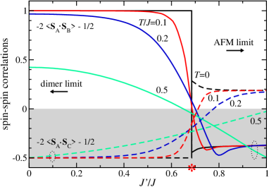
Entanglement in the absence of magnetic field is most prominently reflected in spin-spin correlation functions, e.g., $\langle\textrm{\bf S}_{\mathrm{A}}\cdot\textrm{\bf S}_{\mathrm{B}}\rangle$ and $\langle\textrm{\bf S}_{\mathrm{A}}\cdot\textrm{\bf S}_{\mathrm{C}}\rangle$. In zero temperature limit due to quantum phase transition at $J_{c}^{\prime}$ these correlations change sign. In Fig. 4 are presented renormalized spin-spin correlation functions (for positive values identical to concurrence) as a function of $J^{\prime}/J$: (i) $C_{\mathrm{A}\mathrm{B}}>0$ in dimer phase and (ii) $C_{\mathrm{A}\mathrm{C}}>0$ in the Néel phase. Critical $J^{\prime}_{c}$ is indicated by asterisk. The results for $N=16$ are qualitatively and quantitatively similar to the $N=20$ case presented here. At finite temperatures spin correlations are smeared out as shown in Fig. 4 for various $T$. Limiting Heisenberg case, $J^{\prime}\to\infty$, is discussed in more detail in the next Section. $J^{\prime}=0$ case corresponds to the single dimer limitarnesen01 and Sec. II.

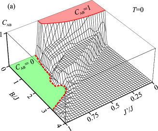
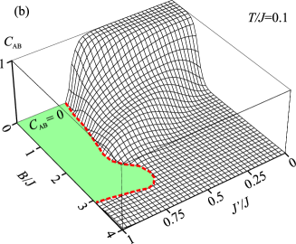
Complete phase diagram of the SSM at $T=0$ but with finite magnetic field can be classified in terms of concurrence instead of spin correlations. In Fig. 5(a)$C_{\mathrm{A}\mathrm{B}}$ is presented as a function of $(J^{\prime}/J,B/J)$ as in the case of a single tetramer, Fig. 2(a). Presented results correspond to the $N=20$ case, while $N=16$ system exhibits very similar structure (not shown here). $N=8$ and $N=4$ cases are qualitatively similar, the main difference being the value of critical $J^{\prime}_{c}$ which increases with $N$. Remarkable similarity between all these cases can be interpreted by local physics in the regime of finite spin gap, $J^{\prime}<J^{\prime}_{c}$. Qubit pairs are there completely entangled, $C_{\mathrm{A}\mathrm{B}}=1$, and $C_{\mathrm{A}\mathrm{B}}\sim{1\over 2}$ for magnetic field larger than the spin gap, but $B<J+2J^{\prime}$. For even larger $B$ concurrence approaches zero, similar to the $N=4$ case. Concurrence is zero also for $J^{\prime}>J^{\prime}_{c}$, except along the $B\sim 4J^{\prime}$ line where weak finite concurrence could be the finite size effect. Similar results are found also for $N=16,8$ cases, and are most pronounced in the $N=4$ case. At finite temperature the structure of concurrence is smeared out [Fig. 5(b)] similar to Fig. 2(b).

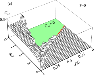
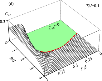
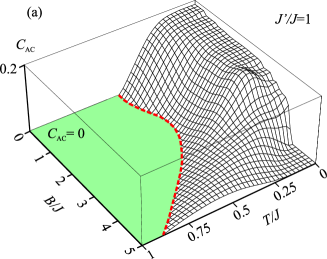
Concurrence $C_{\mathrm{A}\mathrm{C}}$ corresponding to next-nearest neighbors is, complementary to $C_{\mathrm{A}\mathrm{B}}$, increased in the Néel phase of the diagram, Fig. 5(c). The similarity with $N=4$, Fig. 2(c) is somewhat surprising because in this regime long-range correlations corresponding to the gapless spectrum of AFM-like physics are expected to change also short range correlations. The only quantitative difference compared to $N=4$ is the maximum value of $C_{\mathrm{A}\mathrm{C}}\sim 0.3$ instead of $0.5$ (beside the critical value $J^{\prime}_{c}$ discussed in the previous paragraph). Concurrence is very small for $B>J+2J^{\prime}$. At finite temperatures fine fluctuations in the concurrence structure are smeared out, Fig. 5(d).

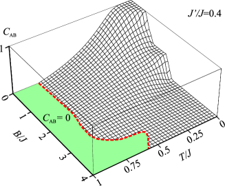
Temperature and magnetic field dependence of $C_{\mathrm{A}\mathrm{B}}$ in the dimer phase is presented in Fig. 6 for fixed $J^{\prime}/J=0.4$. Similarity with the corresponding $N=4$ tetramer case, Fig. 3(a), is astonishing and is again the consequence of local physics in the presence of a finite spin gap. Finite size effects (in comparison with $N=16$ and $N=8$ cases) are very small (not shown). Dashed line represents the borderline of the $C_{\mathrm{A}\mathrm{B}}=0$ region: critical $T_{c}\approx 0.75J$ valid for $B/J\lesssim 3$, that is in this regime nearly independent of $B$, is slightly larger than in the single tetramer case where its insensitivity to $B$ is even more pronounced.

Figure 6: (Color online) Temperature and magnetic field dependence of $C_{\mathrm{A}\mathrm{B}}$ for $J^{\prime}/J=0.4$ and $N=20$. Note the similarity with the corresponding tetramer results, Fig. 3(a). Dashed lines separate $C_{\mathrm{A}\mathrm{B}}>0$ from $C_{\mathrm{A}\mathrm{B}}=0$.

IV Heisenberg limit

The concurrence corresponding to next-nearest neighbors in SSM, $C_{\mathrm{A}\mathrm{C}}$, is non zero in the Néel phase for $J^{\prime}>J^{\prime}_{c}$. Typical result for concurrence in this regime (for fixed $J^{\prime}/J=1$) in terms of temperature and magnetic field is presented in Fig. 7(a). At zero temperature the concurrence is zero for $B>4J^{\prime}$ [compare with Fig. 2(c) and Fig. 5(c)].

In the limit $J=0$ the model simplifies to the AFM Heisenberg model on a square lattice of $N$ sites,

$$H_{\rm AC}=J^{\prime}\sum_{\{\rm AC\}}{\bf S}_{i}\cdot{\bf S}_{j}-B\sum_{i=1}^{N}S_{i}^{z}.$$ (11)

Several results for this model have already been presented for very small clusterswang012 ; cao05 ; zhang05 , however the temperature and magnetic field dependence of the concurrence for systems with sufficiently large number of states and approaching thermodynamic limit has not been presented so far.

Figure 7: (Color online) (a) Next nearest neighbor concurrence $C_{\mathrm{A}\mathrm{C}}$ for $J^{\prime}=J$. (b) Heisenberg lattice result as a special case of the SSM, $J=0$. Shaded region represents $C_{\mathrm{A}\mathrm{C}}=0$. In the line shaded region (low finite temperature and large magnetic field) our numerical results set only the upper limit $C_{\mathrm{A}\mathrm{C}}<5\cdot 10^{-4}$. Dashed lines separate $C_{\mathrm{A}\mathrm{C}}>0$ from $C_{\mathrm{A}\mathrm{C}}=0$.

Figure 8: (Color online) (a) Zero-temperature concurrence $C_{\mathrm{A}\mathrm{C}}$ in the Heisenberg limit as a function of $B/J^{\prime}$ and for various $N=4$, $8$, $16$, $20$. Sections with different total spin values are additionally labeled. (b) Finite-size scaling of concurrence in the absence of magnetic field. Full line represents the fit corresponding to Ref. manousakis, , $C_{\mathrm{A}\mathrm{C}}\approx{1\over 6}+2N^{-3/2}$.

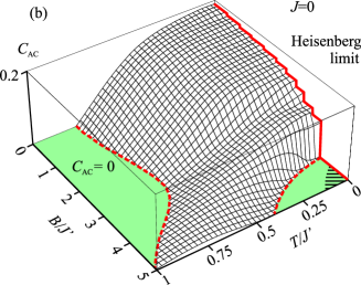
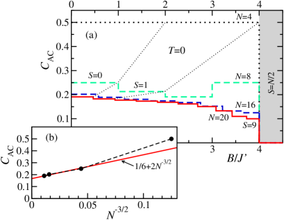
In Fig. 7(b) we further presented temperature and magnetic field dependence of concurrence for the Heisenberg model for $N=20$ (results for $N=16$ are quantitatively similar, but not shown here). Temperature and magnetic field dependence of $C_{\mathrm{A}\mathrm{C}}$ exhibits peculiar semi-island shape where at fixed value of $B$ the concurrence increases with increasing temperature. This effect is to some extent seen in all cases and is the consequence of exciting local singlet states, which do not appear in the ground state. At $T\to 0$ finite steps with increasing $B$ correspond to gradual transition from the singlet ground state to totally polarized state with total spin $S=10$ and vanishing concurrence. This is in more detail presented in Fig. 8(a) for various $N=4,8,16,20$. At $B=0$ and for $N=20$ we get $C_{\mathrm{A}\mathrm{C}}=0.19$. It is interesting to compare this results with the known finite-size analysis scaling for the ground state energy of the Heisenberg model manousakis . The same scaling gives $C_{\mathrm{A}\mathrm{C}}\approx{1\over 6}+2N^{-3/2}$. Our finite-size scaling, Fig. 8(b), is in perfect agreement with this result for $N\to\infty$ at $T=0$ and $B=0$.

In the opposite limit of high magnetic fields, the vanishing concurrence $C_{\rm AC}=0$, is observed for $B$ above the critical value $B_{c}=4J^{\prime}$ for all system sizes shown in Fig. 8(a). This result can be deduced also analytically. Since in a fully polarized state $C_{\rm AC}=0$, this $B_{c}$ actually denotes a transition from $S_{1}=N/2-1$ to $S_{0}=N/2$ ferromagnetic ground state with energy $E_{0}=N(J^{\prime}-B)/2$. The energy of the one-magnon excitation above the ferromagnetic ground state is given by the spin wave theory, which is in this case exact, as $E_{1}=E_{0}-J^{\prime}(2-\cos k_{x}a-\cos k_{y}a)+B$, where $(k_{x},k_{y})$ is the magnon wave vector and $a$ denotes the lattice spacing. Evidently, a transition to a fully polarized state occurs precisely at $B_{c}=4J^{\prime}$ at $(\pi/a,\pi/a)$ point in the one-magnon Brillouin zone.

V Summary

The aim of this paper was to analyze and understand how concurrence (and related entanglement) of qubit pairs (dimers) is affected by their mutual magnetic interactions. In particular, we were interested in a planar array of qubit dimers described by the Shastry-Sutherland model. This model is suitable due to very robust ground state composed of entangled qubit pairs which breaks down by increasing the interdimer coupling. It is interesting to study both, the entanglement between nearest and between next-nearest spins (qubits) at finite temperature and magnetic field. The results are based on numerical calculations using low-temperature Lanczos methods on lattices of 4, 8, 16 and 20 sites with periodic boundary conditions.

A comprehensive analysis of concurrence for various parameters revealed two general conclusions:

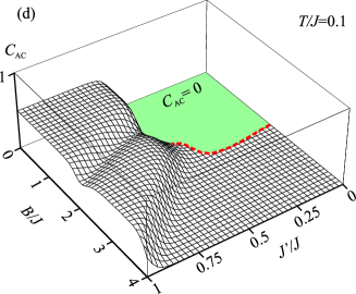
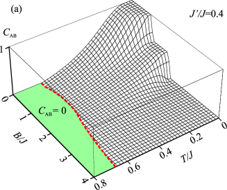
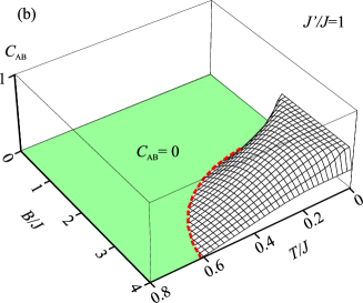
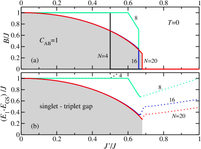
(1) For a weak coupling between qubit dimers, $J^{\prime}<J^{\prime}_{c}$, qubit pairs are locally entangled in accordance with the local nature of the dimer phase. This is due to a finite singlet-triplet gap (spin gap) in the excitation spectrum that is a consequence of strong geometrical frustration in magnetic couplings. The regime of fully entangled neighbors perfectly coincides with the regime of finite spin gap as presented in Fig. 9. Calculated lines for various system sizes $N$ in Fig. 9(a) denote regions (shaded for $N=20$) in the $(J^{\prime}/J,B/J)$ plane where $C_{\mathrm{A}\mathrm{B}}=1$ at $T=0$. In the lower panel [Fig. 9(b)] the lines represent the energy gap $E_{1}-E_{\mathrm{GS}}$ between the first excited state with energy $E_{1}$ with total spin projection $S^{z}=1$ and the ground state with energy $E_{\mathrm{GS}}$ and total spin projection $S^{z}=0$, calculated for $B=0$. For $J^{\prime}<J^{\prime}_{c}$ (full lines) $E_{1}-E_{\mathrm{GS}}$ corresponds to the value of the spin gap. With an increasing magnetic field the spin gap closes (shaded region for $N=20$) and eventually vanishes at the $C_{\mathrm{A}\mathrm{B}}=1$ border line. Shaded regions in Figs. 9(a),(b) therefore coincide. Note also that the results for $N=16$ and 20 sites differ mainly in $J^{\prime}_{c}$.

As a consequence of finite spin gap and local character of correlations it is an interesting observation that even $N=4$ results as a function of temperature and magnetic field qualitatively correctly reproduce $N=20$ results in the regime of $J^{\prime}<J^{\prime}_{c}$. The main quantitative difference is in a renormalized value of $J^{\prime}_{c}=J/2$ for $N=4$, as is evident from the comparison of Figs.2,3 and Figs.5,6. This similarity of the results appears very useful due to the fact that concurrence for tetrahedron-like systems ($N=4$) is given analytically (Sec. II).

(2) In the opposite, strong interdimer coupling regime, $J^{\prime}>J^{\prime}_{c}$, the excitation spectrum is gapless and the concurrence between next-nearest qubits, $C_{\mathrm{A}\mathrm{C}}$, exhibits a similar behavior as in the antiferromagnetic Heisenberg model $J/J^{\prime}\to 0$. Our $B=0$ results coincide with the known result extrapolated to the thermodynamic limit $C_{\mathrm{A}\mathrm{C}}\approx{1\over 6}$. In finite magnetic field and $T=0$ the concurrence vanishes at $B_{c}=4J^{\prime}$ when the system becomes fully polarized (ground state with the total spin $S=N/2$). However, at elevated temperatures the concurrence increases due to excited singlet states and eventually drops to zero at temperatures above $T_{c}\approx J^{\prime}$.

We can conclude with the observation that our analysis of concurrence and related entanglement between qubit pairs was also found to be a very useful measure for classifying various phases of the Shastry-Sutherland model. As our numerical method is based on relatively small clusters, we were unable to unambiguously determine possible intermediate phases of the model in the regime $J^{\prime}\sim J^{\prime}_{c}$, but we believe that concurrence will prove to be a useful probe for the classification of various phases also in this regime using alternative approaches. However, we were able to sweep through all other dominant regimes of the parameters including finite temperature and magnetic field.

VI Acknowledgments

The authors acknowledge J. Mravlje for useful discussions and the support from the Slovenian Research Agency under Contract No. P1-0044.

Figure 9: (Color online) (a) Zero-temperature $C_{\mathrm{A}\mathrm{B}}=1$ region in the plane $(J^{\prime}/J,B/J)$ for various $N$. (b) The corresponding spin gap at $B=0$ (the energy of the lowest total $S^{z}=1$ state relative to the ground state energy).

Appendix A Eigenenergies and eigenvectors for periodically coupled two qubit dimers

Consider two qubit dimers coupled into a tetramer and described with the Hamiltonian Eq. (II) and Fig. 1(a). The model is exactly solvable in the separate $\{S,S^{z}\}$ subspaces corresponding to different values of the total spin $S$ and its $z$ component $S^{z}$. Following the abbreviations for singlet and triplet states on nearest-neighbor (dimer) sites $i$ and $j$,

$$|s_{ij}\rangle = \frac{1}{\sqrt{2}}\,|\!\uparrow_{i}\downarrow_{j}-\downarrow_{i}\uparrow_{j}\rangle,$$

$$|t_{ij}^{0}\rangle = \frac{1}{\sqrt{2}}\,|\!\uparrow_{i}\downarrow_{j}+\downarrow_{i}\uparrow_{j}\rangle,$$

$$|t_{ij}^{+}\rangle = |\!\uparrow_{i}\uparrow_{j}\rangle,$$

$$|t_{ij}^{-}\rangle = |\!\downarrow_{i}\downarrow_{j}\rangle,$$ (12)

the resulting eigenstates $|\phi_{k}\rangle$ and eigenenergies $E_{k}$ corresponding to the hamiltonian Eq. (II) are:

$$S=0, \ S^{z}=0:$$

$$|\phi_{1}\rangle =|s_{\rm AB}\rangle|s_{\rm CD}\rangle,$$

$$E_{1} =-3J/2,$$ (13)

$$|\phi_{2}\rangle =\frac{1}{\sqrt{3}}\big{(}-|t_{\rm AB}^{0}\rangle|t_{\rm CD}^{0}\rangle+|t_{\rm AB}^{+}\rangle|t_{\rm CD}^{-}\rangle+|t_{\rm AB}^{-}\rangle|t_{\rm CD}^{+}\rangle\big{)}$$

$$E_{2} =J/2-4J^{\prime}.$$ (14)

$$S=1, \ S^{z}=-1:$$

$$|\phi_{3}\rangle =|s_{\rm AB}\rangle|t_{\rm CD}^{-}\rangle,$$

$$|\phi_{4}\rangle =|t_{\rm AB}^{-}\rangle|s_{\rm CD}\rangle,$$

$$E_{3,4} =-J/2-B,$$ (15)

$$|\phi_{5}\rangle =\frac{1}{\sqrt{2}}\big{(}|t_{\rm AB}^{0}\rangle|t_{\rm CD}^{-}\rangle-|t_{\rm AB}^{-}\rangle|t_{\rm CD}^{0}\rangle\big{)},$$

$$E_{5} =J/2-2J^{\prime}-B.$$ (16)

$$S=1, \ S^{z}=0:$$

$$|\phi_{6}\rangle =|s_{\rm AB}\rangle|t_{\rm CD}^{0}\rangle,$$

$$|\phi_{7}\rangle =|t_{\rm AB}^{0}\rangle|s_{\rm CD}\rangle,$$

$$E_{6,7} =-J/2,$$ (17)

$$|\phi_{8}\rangle =\frac{1}{\sqrt{2}}\big{(}|t_{\rm AB}^{+}\rangle|t_{\rm CD}^{-}\rangle-|t_{\rm AB}^{-}\rangle|t_{\rm CD}^{+}\rangle\big{)},$$

$$E_{8} =J/2-2J^{\prime}.$$ (18)

$$S=1, \ S^{z}=1:$$

$$|\phi_{9}\rangle =|s_{\rm AB}\rangle|t_{\rm CD}^{+}\rangle,$$

$$|\phi_{10}\rangle =|t_{\rm AB}^{+}\rangle|s_{\rm CD}\rangle,$$

$$E_{9,10} =-J/2+B,$$ (19)

$$|\phi_{11}\rangle =\frac{1}{\sqrt{2}}\big{(}-|t_{\rm AB}^{0}\rangle|t_{\rm CD}^{+}\rangle+|t_{\rm AB}^{+}\rangle|t_{\rm CD}^{0}\rangle\big{)},$$

$$E_{11} =J/2-2J^{\prime}+B.$$ (20)

$$S=2, \ S^{z}=-2:$$

$$|\phi_{12}\rangle =|t_{\rm AB}^{-}\rangle|t_{\rm CD}^{-}\rangle,$$

$$E_{12} =J/2+2J^{\prime}-2B.$$ (21)

$$S=2, \ S^{z}=-1:$$

$$|\phi_{13}\rangle =\frac{1}{\sqrt{2}}\big{(}|t_{\rm AB}^{0}\rangle|t_{\rm CD}^{-}\rangle+|t_{\rm AB}^{-}\rangle|t_{\rm CD}^{0}\rangle\big{)},$$

$$E_{13} =J/2+2J^{\prime}-B.$$ (22)

$$S=2, \ S^{z}=0:$$

$$|\phi_{14}\rangle =\frac{1}{2}\big{(}2|t_{\rm AB}^{0}\rangle|t_{\rm CD}^{0}\rangle+|t_{\rm AB}^{+}\rangle|t_{\rm CD}^{-}\rangle+|t_{\rm AB}^{-}\rangle|t_{\rm CD}^{+}\rangle\big{)},$$

$$E_{14} =J/2+2J^{\prime}.$$ (23)

$$S=2, \ S^{z}=1:$$

$$|\phi_{15}\rangle =\frac{1}{\sqrt{2}}\big{(}|t_{\rm AB}^{0}\rangle|t_{\rm CD}^{+}\rangle+|t_{\rm AB}^{+}\rangle|t_{\rm CD}^{0}\rangle\big{)},$$

$$E_{15} =J/2+2J^{\prime}+B.$$ (24)

$$S=2, \ S^{z}=2:$$

$$|\phi_{16}\rangle =|t_{\rm AB}^{+}\rangle|t_{\rm CD}^{+}\rangle,$$

$$E_{16} =J/2+2J^{\prime}+2B.$$ (25)

References

- (1) M. A. Nielsen and I. A. Chuang, Quantum Information and Quantum Computation (Cambridge University Press, Cambridge, 2001).
- (2) A. Osterloh, L. Amico, G. Falci, and R. Fazio, Nature 416, 608 (2002).
- (3) C. H. Bennett, H. J. Bernstein, S. Popescu, and B. Schumacher, Phys. Rev. A 53, 2046 (1996); C. H. Bennett, D. P. DiVincenzo, J. A. Smolin, and W.K. Wootters, ibid. 54, 3824 (1996).
- (4) S. Hill and W. K. Wootters, Phys. Rev. Lett. 78, 5022 (1997).
- (5) V. Vedral, M. B. Plenio, M. A. Rippin, and P. L. Knight, Phys. Rev. Lett. 78, 2275 (1997).
- (6) W. K. Wootters, Phys. Rev. Lett. 80, 2245 (1998).
- (7) J. Schliemann, D. Loss, and A. H. MacDonald, Phys. Rev. B 63, 085311 (2001); J. Schliemann, J. I. Cirac, M. Kuś, M. Lewenstein, and D. Loss, Phys. Rev. A 64, 022303 (2001).
- (8) G.C. Ghirardi and L. Marinatto, Phys. Rev. A 70, 012109 (2004).
- (9) K. Eckert, J. Schliemann, G. Brus, and M. Lewenstein, Ann. Phys. 299, 88 (2002).
- (10) J. R. Gittings and A. J. Fisher, Phys. Rev. A 66 032305 (2002).
- (11) P. Zanardi, Phys. Rev. A 65, 042101 (2002).
- (12) V. Vedral, Cent. Eur. J. Phys. 2, 289 (2003); D. Cavalcanti, M. F. Santos, M. O. TerraCunha, C. Lunkes, V. Vedral, Phys. Rev. A 72, 062307 (2005).
- (13) D. P. DiVincenzo, Mesoscopic Electron Transport, NATO Advanced Studies Institute, Series E: Applied Science, edited by L. Kouwenhoven, G. Schön, and L. Sohn (Kluwer Academic, Dordrecht, 1997); cond-mat/9612126.
- (14) D. P. DiVincenzo, Science 309, 2173 (2005).
- (15) W. A. Coish and D. Loss, cond-mat/0603444.
- (16) J. M. Elzerman, R. Hanson, J. S. Greidanus, L. H. Willems van Beveren, S. DeFranceschi, L. M. K. Vandersypen, S. Tarucha, and L. P. Kouwenhoven, Phys. Rev. B 67, 161308 (2003).
- (17) J. C. Chen, A. M. Chang, and M. R. Melloch, Phys. Rev. Lett. 92, 176801 (2004).
- (18) T. Hatano, M. Stopa, and S. Tarucha, Science 309, 268 (2005).
- (19) J. R. Petta, A. C. Johnson, J. M. Taylor, E. A. Laird, A. Yacoby, M. D. Lukin, C. M. Marcus, M. P. Hanson, and A. C. Gossard, Science 309, 2180 (2005).
- (20) M. A. Nielsen, Ph.D. thesis, University of New Mexico, 1998; quant-ph/0011036.
- (21) M. C. Arnesen, S. Bose, and V. Vedral, Phys. Rev. Lett. 87, 017901 (2001).
- (22) X. Wang, Phys. Lett. A 281, 101 (2001).
- (23) B. V. Fine, F. Mintert, and A. Buchleitner Phys. Rev. B 71, 153105 (2005).
- (24) A. Ramšak, J. Mravlje, R. Žitko, and J. Bonča, Phys. Rev. B 74, 241305(R) (2006).
- (25) T. Yu and J. H. Eberly, Phys. Rev. B 66, 193306 (2002).
- (26) B. S. Shastry and B. Sutherland, Physica B 108, 1069 (1981).
- (27) O. F. Syljuåsen, Phys. Rev. A 68, 060301(R) (2003)
- (28) L. Amico, A. Osterloh, F. Plastina, R. Fazio, and G.M. Palma, Phys. Rev. A 69, 022304 (2004).
- (29) T. J. Osborne and M. A. Nielsen, Phys. Rev. A 66, 032110 (2002).
- (30) T. Roscilde, P. Verrucchi, A. Fubini, S. Haas, and V. Tognetti, Phys. Rev. Lett. 93, 167203 (2004).
- (31) T. Roscilde, P. Verrucchi, A. Fubini, S. Haas, and V. Tognetti, Phys. Rev. Lett. 94, 147208 (2005).
- (32) D. Larsson and H. Johannesson, Phys. Rev. Let. 95, 196406 (2005).
- (33) Shi-Jian Gu, Shu-Sa Deng, You-Quan Li, and Hai-Qing Lin Phys. Rev. Lett. 93, 086402 (2004).
- (34) S. S. Deng, S. J. Gu, and H. Q. Lin Phys. Rev. B 74, 045103 (2006).
- (35) Ö. Legeza and J. Sólyom, Phys. Rev. Lett. 96, 116401 (2006).
- (36) F. Verstraete, M. Popp, and J. I. Cirac, Phys. Rev. Lett. 92, 027901 (2004).
- (37) A. Ramšak, I. Sega, and J. H. Jefferson Phys. Rev. A 74, 010304(R) (2006).
- (38) R. F. Werner, Phys. Rev. A 40, 4277 (1989).
- (39) I. Bose and A. Tribedi, Phys. Rev. A 72, 022314 (2005).
- (40) R. W. Smith and D. A. Keszler, J. Solid State Chem. 93, 430 (1991).
- (41) H. Kageyama, K. Yoshimura, R. Stern, N. V. Mushnikov, K. Onizuka, M. Kato, K. Kosuge, C. P. Slichter, T. Goto, and Y. Ueda, Phys. Rev. Lett. 82, 3168 (1999).
- (42) S. Miyahara and K. Ueda, J. Phys.: Condens. Matter 15, R327 (2003); and references therein.
- (43) G. A. Jorge, R. Stern, M. Jaime, N. Harrison, J. Bonča, S. El Shawish, C. D. Batista, H. A. Dabkowska, and B. D. Gaulin, Phys Rev. B 71, 092403 (2005).
- (44) S. El Shawish, J. Bonča, C. D. Batista, and I. Sega, Phys. Rev. B 71, 014413 (2005).
- (45) S. El Shawish, J. Bonča, and I. Sega, Phys. Rev. B 72, 184409 (2005).
- (46) S. Miyahara and K. Ueda, Phys. Rev. Lett. 82, 3701 (1999).
- (47) E. Müller-Hartmann, R. R. P. Singh, C. Knetter, and G. S. Uhrig, Phys. Rev. Lett. 84, 1808 (2000).
- (48) A. Isacsson and O. F. Syljuåsen, Phys. Rev. E 74, 026701 (2006); and references therein.
- (49) K. Onizuka, H. Kageyama, Y. Narumi, K. Kindo, Y. Ueda, and T. Goto, J. Phys. Soc. Jpn. 69, 1016 (2000).
- (50) T. Momoi and K. Totsuka, Phys. Rev. B 61, 3231 (2000).
- (51) G. Misguich, Th. Jolicoeur, and S. M. Girvin, Phys. Rev. Lett., 87, 097203 (2001).
- (52) M. Aichhorn, M. Daghofer, H. G. Evertz, and W. von der Linden, Phys. Rev. B 67, 161103(R) (2003).
- (53) J. Jaklič and P. Prelovšek, Adv. Phys. 49, 1 (2000); Phys. Rev. Lett. 77, 892 (1996); Phys. Rev. B 49, 5065 (1994).
- (54) J. Bonča and P. Prelovšek, Phys. Rev. B 67, 085103 (2003).
- (55) X. Wang, Phys. Rev. A 64, 012313 (2001); ibid. 66, 044305 (2002).
- (56) M. Cao and S. Zhu, Phys. Rev. A 71, 034311 (2005).
- (57) G. F. Zhang and S. S. Li, Phys. Rev. A 72, 034302 (2005).
- (58) E. Manousakis, Rev. Mod. Phys. 63, 1 (1991).