Radiative losses and cut-offs of energetic particles at relativistic shocks

Abstract

We investigate the acceleration and simultaneous radiative losses of electrons in the vicinity of relativistic shocks. Particles undergo pitch angle diffusion, gaining energy as they cross the shock by the Fermi mechanism and also emitting synchrotron radiation in the ambient magnetic field. A semi-analytic approach is developed which allows us to consider the behaviour of the shape of the spectral cut-off and the variation of that cut-off with the particle pitch angle. The implications for the synchrotron emission of relativistic jets, such as those in gamma ray burst sources and blazars, are discussed.

1 Introduction

The role of radiative losses in determining the spectra from non-thermal sources has been well understood in the non-relativistic shock limit since the work of Webb et al. (1984) and Heavens & Meisenheimer (1987). Their results were in broad agreement with the natural expectation that there would be a cut-off in the spectrum, at the shock, and at a momentum where acceleration and loss timescales are equal, with the shape of this cut-off depending critically on the momentum dependence of the particle scattering. Subsequently, as the particles are advected downstream, and are no longer efficiently accelerated by the shock, the spectra steepens at momenta where the particles have had sufficient time to cool. At a strong, nonrelativistic shock the differential number density of particles at energies where radiative cooling is unimportant is a power law with $N(E)\propto E^{-0.5}$ with a corresponding intensity of $I_{\nu}\propto\nu^{-0.5}$ for the emitted synchrotron radiation. At higher momenta, where cooling becomes important, the spectrum steepens so that the radiation, beyond a break frequency $\nu_{b}$, is $I_{\nu}\propto\nu^{-1}$ up to a critical frequency, $\nu_{c}$ corresponding to cut-off of the particle spectrum. The position of $\nu_{b}$ depends on position away from the shock; decreasing downstream as the particles have more time to cool. The observed emission is therefore dependent on the spatial resolution with which the source is observed as discussed in Heavens & Meisenheimer (1987). The results in the existing literature refer only to non-relativistic flows and are of great use in analysing the spectra from supernovae and the jets of some active galaxies (AGN). However, a number of objects of astrophysical importance, such as AGN jets, microquasars and gamma-ray bursts, contain flows which have bulk relativistic motion and the purpose of this paper is to examine the breaks, cut-offs and emission for such sources.

While the first order Fermi process at relativistic shocks contains the same basic physics as in the nonrelativistic case, i.e. scattering leading to multiple shock crossings competing with a finite chance of escape downstream, the anisotropy of the particle distribution complicates the analysis considerably (Kirk & Schneider (1987), Heavens & Drury (1988) and Kirk et al. (2000)). The inclusion of self-consistent synchrotron losses will, as in the nonrelativistic limit, modify the spectrum at high momenta but we would also expect pitch angle effects to become apparent in the position of the cut-off and the emission itself. In order to motivate our treatment of this problem we first discuss the nonrelativistic shock limit in section 2, including the emission from a spatially integrated source. Section 3 then presents the analysis of synchrotron losses at relativistic shocks with particular emphasis on the shape of the momentum cut-off. We conclude with a discussion in section 4.

2 Nonrelativistic Shocks

The effect of synchrotron losses on the energetic particle distribution in the presence of nonrelativistic shocks is demonstrated rigorously in Webb et al. (1984). However a simpler approach is described in Heavens & Meisenheimer (1987) provided synchrotron losses are not considered important at the injection energies. We will follow this approach here, although we shall introduce a slightly different definition of the cut-off momentum.

In the presense of a magnetic field charged particles emit synchrotron radiation with an energy loss rate given by

$$\frac{dp}{dt}=-a_{s}B^{2}p^{2}=-\lambda p^{2}$$ (1)

where $a_{s}$ is a positive constant. The radiative loss timescale is therefore $t_{\rm loss}=1/(\lambda p)$. In the steady state, and in the presence of a nonrelativistic flow $u$, energetic particles obey a transport equation describing advection, diffusion, adiabatic compression and radiative losses,

$$u\frac{\partial f}{\partial z}-\frac{\partial}{\partial z}\left(\kappa\frac{\partial f}{\partial z}\right){-\frac{1}{3}p\frac{\partial u}{\partial z}\frac{\partial f}{\partial p}}-\frac{1}{p^{2}}\frac{\partial}{\partial p}\left(\lambda p^{4}f\right)=0.$$ (2)

In the presence of a nonrelativistic shock front where the upstream flow speed is $u_{-}$ and that downstream is $u_{+}$ the acceleration timescale is

$$t_{\rm acc}=\frac{3}{u_{-}-u_{+}}\left(\frac{\kappa_{-}}{u_{-}}+\frac{\kappa_{+}}{u_{+}}\right).$$ (3)

At momenta for which $t_{\rm acc}\ll t_{\rm loss}$ the phase space density will be a simple power law with $f\propto p^{-s}$ where $s=3u_{-}/(u_{-}-u_{+})$.

2.1 Momentum Cut-off

The spectrum will steepen at momentum $p^{*}$ where $t_{\rm acc}(p^{*})=t_{\rm loss}(p^{*})$. In the case of momentum independent diffusion this gives

$$p^{*}=\frac{u_{-}-u_{+}}{3}\left({\frac{\lambda_{-}\kappa_{-}}{u_{-}}}+\frac{\lambda_{+}\kappa_{+}}{u_{+}}\right)^{-1}.$$ (4)

In the case of a relativistic shock this result no longer strictly holds since the acceleration timescale defined above is only valid for nonrelativistic flows. Nevertheless, we will use this definition of $p^{*}$ throughout the paper for the sake of comparison.

However, we require a general definition of the cut-off momentum that can be applied in the relativistic limit. An obvious alternative is to define the momentum at which the local spectral index, $\partial\ln f/\partial\ln p$, becomes $s+1$ but, as we shall see, it is necessary to perform a Laplace transform of the transport equation to proceed with this problem and it is more straightforward to define the cut-off in terms of spectral steepening of the Laplace transformed spectrum. In order to motivate such a definition we solve the nonrelativistic shock acceleration problem in the presence of synchrotron losses by first making the substitutions $W\equiv p^{4}f$ and $y\equiv 1/p$ so that the transport equation, either upstream or downstream of the shock where adiabatic losses are zero, becomes

$$u\frac{\partial W}{\partial z}-\frac{\partial}{\partial z}\left(\kappa\frac{\partial W}{\partial z}\right)+\frac{\partial}{\partial y}\left(\lambda W\right)=0.$$ (5)

Taking the Laplace transform with respect to $y$

$${\hat{W}}(k,z)=\int_{0}^{\infty}W(y,z)\exp(-yk)dy$$ (6)

and using the fact that losses prevent any particles achieving infinite energy, i.e. $W(0,z)=0$, the transformed transport equation is

$$u\frac{\partial{\hat{W}}}{\partial z}-\frac{\partial}{\partial z}\left(\kappa\frac{\partial{\hat{W}}}{\partial z}\right)+\lambda k{\hat{W}}=0.$$ (7)

in the case of a momentum independent diffusion coefficient. Since the distribution function must be bounded infinitely far upstream and downstream, the solution becomes

$${\hat{W}}_{\pm}=A_{\pm}(k)\exp\left(\frac{1{\mp}\sqrt{1+\omega_{\pm}k}}{2}\frac{u_{\pm}}{\kappa_{\pm}}z\right)$$ (8)

where we have introduced

$$\omega_{\pm}\equiv\frac{4\lambda_{\pm}\kappa\pm}{u_{\pm}^{2}}.$$ (9)

The isotropic and anisotropic parts of the particle distribution function must match up at the shock giving,

$$f_{-}(p,0) =f_{+}(p,0)$$ (10)

$$\kappa_{-}\frac{\partial f_{-}}{\partial z}+\frac{u_{-}}{3}p\frac{\partial f_{-}}{\partial p} =\kappa_{+}\frac{\partial f_{+}}{\partial z}+\frac{u_{+}}{3}p\frac{\partial f_{+}}{\partial p}.$$ (11)

Multiplying the isotropic boundary condition by $p^{4}$, making the substitutions as above and taking the Laplace transform with respect to $1/p$ gives

$${\hat{W}}_{-}(k,z=0)={\hat{W}}_{+}(k,z=0)$$ (12)

which in turn gives

$$A_{-}(k)=A_{+}(k)\equiv A(k).$$ (13)

The flux continuity condition (11) becomes

$$A(k)=A_{0}k^{3-s}\exp\left(-s\sqrt{1+\omega_{-}k}-(s-3)\sqrt{1+\omega_{+}k}\right)\times$$

$$\left(1+\sqrt{1+\omega_{-}k}\right)^{s}\left(1+\sqrt{1+\omega_{+}k}\right)^{s-3}.$$ (14)

In the absence of synchrotron losses, $\omega_{\pm}=0$, we have ${\hat{W}}_{\pm}(k)\propto k^{3-s}$ which, upon inversion, gives $f(p)\propto p^{-s}$ as expected. We can therefore define a function, ${\hat{Q}}$, by ${\hat{W}}=k^{3-s}{\hat{Q}}$. Recalling that $k$ is the Laplace transformed variable of inverse momentum we define the cut-off momentum, $p_{\rm cut}$, to occur at the point where

$$\left.\frac{\partial\ln{\hat{Q}}}{\partial\ln k}\right|_{k=p_{\rm cut}}=-1.$$ (15)

As an illustrative example, consider a power law distribution with a sharp maximum momentum, $f(p)\propto p^{-s}H(p_{\rm max}-p)$ with $H$ the Heaviside function. In this case we have

$$W=y^{s-4}H\left(y-\frac{1}{p_{\rm max}}\right)\;\;\;\Rightarrow\;\;\;{\hat{W}}=e^{-\frac{k}{p_{\rm max}}}\Gamma(s-3)k^{3-s}$$ (16)

where $\Gamma$ is the Gamma function. With ${\hat{Q}}\propto\exp(-k/p_{\rm max})$ we then have $p_{\rm cut}=p_{\rm max}$ as required physically in this simple case.

Returning to the solution of the shock problem we have from equation 2.1

$$\left.{\hat{Q}}\right|_{z=0}=\exp\left(-s\sqrt{1+\omega_{-}k}-(s-3)\sqrt{1+\omega_{+}k}\right)$$

$$\times\left(1+\sqrt{1+\omega_{-}k}\right)^{s}\left(1+\sqrt{1+\omega_{+}k}\right)^{s-3}.$$ (17)

Defining

$$\Omega =\omega_{+}/\omega_{-}$$ (18)

$$\chi =\sqrt{\left({s}^{2}+2\,\,{s}^{2}{\Omega}+{{\Omega}}^{2}{s}^{2}-6\,{{\Omega}}^{2}s+2\,{\Omega}\,s+9\,{{\Omega}}^{2}-8\,{\Omega}\,\right)}$$

$$\qquad\times\left(s-3\right)$$ (19)

gives

$$p_{\rm cut}=\frac{2}{\omega_{-}}\Bigg{(} \frac{s^{4}(2+2\Omega)-s^{3}(5+11\Omega)+s^{2}(5+8\Omega-2\chi)}{\left(s^{2}(1-\Omega)+6\Omega s-9\Omega\right)^{2}}$$

$$+\frac{s(33\Omega+\chi)-36\Omega}{\left(s^{2}(1-\Omega)+6\Omega s-9\Omega\right)^{2}}\Bigg{)}.$$ (20)

This is always greater than $p^{*}$,

$$p^{\ast}=\frac{4}{\omega_{-}}\frac{1}{s+(s-3)\Omega}$$ (21)

as can be seen from figure 1. The minimum value for $p_{\rm cut}$ occurs for $\Omega=1$, and is given by $p_{\rm cut}=\frac{2(s-1)}{2s-3}p^{\ast}$.

Figure 1: The cut-off momentum, $p_{\rm cut}$ as a function of $\Omega$ for fixed equilibrium momentum, $p^{\ast}=1$, and spectral index, $s=4$.

The Laplace inversion (see Appendix for details) for $s=4$ and $\Omega=1$ is shown in figure 2. Using just $M=6$ in the Salzer summation the inversion has already converged. The first approximation $M=1$ is exactly the Laplace function $\hat{W}k$. We can see how fast the Salzer summation Post-Widder inversion converges as $M=2$ is a good approximation to the actual solution.

Figure 2: Laplace inversion for $s=4$ and $\Omega=1$. Using just $M=6$ in the Salzer summation the inversion has already converged. The first approximation $M=1$ is exactly the Laplace function $\hat{W}k$. We can see how fast the Salzer summation Post-Widder inversion converges as $M=2$ is a very reasonably approximation to the actual solution.

Figure 3 shows how the particle distribution varies with $\Omega$; if $\Omega\neq 1$ the cut-off is broader. While $p^{\ast}$ is independent of $\Omega$, $p_{\rm cut}$ increases as the distribution broadens.

Figure 3: Particle Distributions of Various $\Omega$

The data in figure 3 can be fitted by an exponential tail to the distribution of the form

$$\exp\left(-\left({p}/{p_{\rm cut}}\right)^{\beta}\right)$$ (22)

where $\beta\sim 2$. Table 1 shows how $\beta$ varies with $\Omega$ for a shock of natural spectral index $s=4$, with $\beta$ attaining its maximum value of $2.25$, i.e. the cut-off is sharpest, when $\Omega=1$. When $\Omega\gg 1$ particles can diffuse in the upstream without losing any energy, allowing a greater spread in momentum above $p_{\rm cut}$.

$\Omega$	$p^{\ast}$	$p_{\rm cut}$	$\beta$
0	1	1.25	2.25
1	1	1	2.25
9	1	1.4	2
16	1	1.53	1.8
25	1	1.63	1.75
$\infty$	1	2	1.5

Table 1: Parameters for fitting particle spectra

Figure 4: The spatial variation of the particle distribution for $\Omega=1$. $z^{\prime}=\frac{u_{+}}{\kappa_{+}}z$.

Figure 5: The spatially integrated particle distribution for $\Omega=1$ from $z^{\prime}=0$ to $z^{\prime}=50$. Note that as well as the particle cut-off there is a spectral break earlier were they spectrum softens from $p^{-4}$ to $p^{-5}$. This is analogous to synchrotron ageing.

2.2 The Integrated Distribution Function and Synchrotron Spectra

When the source cannot be fully resolved observationally, we must include the contribution from all particles within some distance $z^{\prime}$ of the shock in calculating the spatially integrated emission. In the case of steady emission from a jet pointing towards us, or a completely unresolved source, $z^{\prime}$ is essentially the source size in the optically thin limit. For simplicity we assume that the magnetic field downstream of the shock is constant although the model can be generalised for more complex cases.

The integrated Laplace distribution function is

$$\hat{T} =\int_{0}^{z^{\prime}}\hat{W}\;dz$$

$$=\frac{A_{0}\kappa_{+}}{u_{+}}\frac{k^{3-s}\left.{\hat{Q}}\right|_{z=0}\left(1+\sqrt{1+\omega_{+}k}\right)}{\omega_{+}k}$$

$$\qquad\times\left(1-\exp\left(\frac{1-\sqrt{1+\omega_{+}k}}{2}\frac{u_{+}}{\kappa_{+}}z^{\prime}\right)\right).$$ (23)

When $z^{\prime}$ is very small the result is $k^{3-s}$ with a cut-off at high $k$ as expected. As $z^{\prime}$ tends to infinity at low $k$ we have $k^{2-s}$ so the spectrum is steepened , with the same high $k$ cut-off. For finite values of $z^{\prime}$ the spectrum starts as $k^{3-s}$ before turning into $k^{2-s}$ and finally cutting off. We shall see later that this result also holds in real momentum space.

Figure 4 shows how the cut-off tends to lower momenta as we go further downstream. However what is most often observed a result of the integrated distribution is shown in figure 5. While the cut-off momentum is the same as at the shock, the distribution changes from an initial $p^{-4}$ to a $p^{-5}$ spectrum at some critical momentum, $p_{\rm b}$, which depends on $z^{\prime}$. Here we will consider only synchrotron emission from an ordered magnetic field (parallel to the flow). Let $w=\frac{4\pi\nu m_{e}^{3}c^{2}}{3qB}$ where $\nu$ is the frequency, $q$ is the charge on the electron, $m_{e}$ is the electron mass and $B$ is the magnetic field strength. Then given a spatially integrated particle distribution $f\propto p^{-s}g(p,\mu)$ the total power emitted per unit frequency is (Rybicki & Lightman, 1986)

$$P_{tot}(\omega)\propto\sqrt{1-\mu^{2}} \int_{0}^{\infty}\left(\frac{w}{x\sqrt{1-\mu^{2}}}\right)^{(s-5)/2}$$

$$g\left(\sqrt{\frac{w}{x\sqrt{1-\mu^{2}}}},\mu\right)F(x)\;dx$$ (24)

where $F$ is the first synchrotron function

$$F(x)\equiv x\int_{x}^{\infty}K_{\frac{5}{3}}(y)\;dy.$$ (25)

In the case of non-relativistic diffusive shock acceleration $f$ downstream of a shock is assumed to be isotropic in which case $g$ is independent of $\mu$.

Figure 6: A telescope with very high resolution may be able to observe synchrotron radiation at the shock. The only spectral feature here is the cut-off at $\nu_{\rm cut}$. Before $\nu_{\rm cut}$ the spectrum has shape $I(\nu)\sim\nu^{-1/2}$. For this result $\Omega=1$.

Figure 7: Spatially integrated emission for $\Omega=1$. The black dashed curve shows the synchrotron spectrum of an unresolved object containing a strong shock. The only feature is the spectral cut-off at $\nu_{\rm cut}$. Before $\nu_{\rm cut}$ the spectrum has shape $I(\nu)\sim\nu^{-1}$. The solid curve illustrates the synchrotron spectrum of a partially resolved source with emission from the shock ($z^{\prime}=0$) to some downstream distance ($z^{\prime}=50$).

Figure 6 shows the emission at the shock. The only feature here is the cut-off hump, which is of course related to the particle cut-off, before which $I_{\nu}\sim\nu^{-(s-3)/2}$. Figure 7 shows a more realistic plot, that of emission from an extended region. If the region is infinite in size then the cut-off remains the sole feature but the spectrum before the cut-off is different $I_{\nu}\sim\nu^{-(s-2)/2}$. If the region has finite size then a second feature, the spectral break $\nu_{b}$, appears. Before the break the spectrum goes as $I_{\nu}\sim\nu^{-(s-3)/2}$ while after it it is $I_{\nu}\sim\nu^{-(s-2)/2}$. Again this is related to the momentum break $p_{b}$ we see in the particle distribution in figure 5.

3 Relativistic Shock Acceleration with Losses

In the case of a relativistic shock, the particle transport equation describing advection, pitch angle diffusion and losses becomes

$$\Gamma\,(u+\mu)\frac{\partial f}{\partial z}=\frac{\partial}{\partial\mu}\left(D_{\mu\mu}\frac{\partial f}{\partial\mu}\right)+\lambda g(\mu)\frac{1}{p^{2}}\frac{\partial(p^{4}f)}{\partial p}$$ (26)

where $\mu$ is the cosine of the pitch angle of the particle and the flow velocity is constant upstream and downstream of the shock. $\lambda=\frac{2\sigma_{T}}{m^{2}c^{2}}U_{B}$ and $g(\mu)=1-\mu^{2}$ for synchrotron losses in an ordered magnetic field, $\lambda=4\sigma_{\rm T}U_{\rm B}/3$ and $g(\mu)=1$ for synchrotron losses in a tangled magnetic field, or $\lambda=4\sigma_{\rm T}U_{\rm rad}/3$ and $g(\mu)=1$ for inverse Compton losses. Equation (26) holds separately upstream and downstream with the conditions that the distribution is isotropic infinity far downstream, there are no particles infinitely far upstream and the distribution is continuous at the shock. Although we will derive equations for general momentum independent pitch-angle diffusion and an arbitrary magnetic field alignment, the figures and results produced throughout the rest of this paper are for isotropic diffusion $D_{\mu\mu}=D(1-\mu^{2})$ in an ordered (longitudinal) magnetic field with $\lambda/D=0.1$.

Guided by the treatment of the nonrelativistic case we set $W=p^{4}f$ and $y=1/p$ so that

$$\Gamma(u+\mu)\frac{\partial W}{\partial z}= \frac{\partial}{\partial\mu}\left[D(\mu)(1-\mu^{2})\frac{\partial W}{\partial\mu}\right]-{\lambda}g(\mu)\frac{\partial W}{\partial y}.$$ (27)

Taking the Laplace Transform with respect to $y$ and assuming $W(0,\mu,z)=0$

$$\Gamma(u+\mu)\frac{\partial{\hat{W}}}{\partial z}= \frac{\partial}{\partial\mu}\left[D(\mu)(1-\mu^{2})\frac{\partial{\hat{W}}}{\partial\mu}\right]-{\lambda}g(\mu){k{\hat{W}}}.$$ (28)

With the spatial and pitch angle variables separable we look for solutions of the form

$${\hat{W}}(k,\mu,z)=\sum_{i}a_{i}(k)X_{i}(k,z)Q_{i}(k,\mu)$$ (29)

putting this back into the reduced transport equation we get

$$\Gamma(u+\mu)\frac{\partial X_{i}}{\partial z}Q_{i}=(\overline{\mathcal{D}}Q_{i})X_{i}$$ (30)

where we have defined the differential operator $\overline{\mathcal{D}}$ via

$$\overline{\mathcal{D}}\Phi=\frac{\partial}{\partial\mu}\left[D(\mu)(1-\mu^{2})\frac{\partial\Phi}{\partial\mu}\right]-\lambda g(\mu)k\Phi.$$ (31)

Separating $X$ and $Q$ we get the usual

$$\Gamma\frac{1}{X_{i}}\frac{\partial X_{i}}{\partial z}=\Lambda_{i}(k)=\frac{1}{Q_{i}(u+\mu)}\overline{\mathcal{D}}Q_{i}$$ (32)

$$\Rightarrow X_{i}(k,z)=\exp\left(\frac{\Lambda_{i}(k)z}{\Gamma}\right)$$ (33)

and we have an equation for $Q(k,\mu)$

$${\overline{\mathcal{D}}Q_{i}-\Lambda_{i}(k)Q_{i}(u+\mu)=0.}$$ (34)

Expanding out the differential operator we get

$$\frac{\partial}{\partial\mu}\left(D(\mu)(1-\mu^{2})\frac{\partial Q_{i}}{\partial\mu}\right)-\left(\Lambda_{i}(u+\mu)+k\lambda g(\mu)\right)Q_{i}=0$$ (35)

which has regular singularities at $\mu=\pm 1$ and so it should be possible to find solutions for $Q_{i}$ on $[-1,1]$ for all $k\in\mathbb{C}$.

3.1 Determining the Eigenfunctions

We know that along the real axis, $k=x\in\mathbb{R}$, each $Q_{i}$ satisfies

$$\frac{\partial}{\partial\mu}\left(D(\mu)(1-\mu^{2})\frac{\partial Q_{i}}{\partial\mu}\right)-\left(\Lambda_{i}(u+\mu)+x\lambda g(\mu)\right)Q_{i}=0.$$ (36)

We define an inner product by:

$$\langle\zeta,\xi\rangle=\int(u+\mu){\zeta}^{*}\xi d\mu.$$ (37)

It can be shown that the $Q_{i}(x)$ are orthogonal and either real or purely imaginary, and the $\Lambda_{i}(x)$ are real and distinct. We can normalise the eigenfunctions such that

$$\langle Q_{i},Q_{j}\rangle=\delta_{i,j}$$ (38)

or considering them as real

$$\langle Q_{i},Q_{j}\rangle=\delta_{i,j}{\left(1/2-i\right)/\left|{1}/{2}-i\right|}\equiv\eta_{i,j}.$$ (39)

Then we have (see Appendix for details)

$$\frac{\partial Q_{i}}{\partial x}=\lambda\sum_{j\not=i}\frac{1}{\Lambda_{j}-\Lambda_{i}}\left(\int g(\mu)Q_{i}{Q_{j}}d\mu\right)Q_{j}\eta_{j,j}$$ (40)

and

$$\frac{d\Lambda_{i}}{dx}=-\lambda\left(\int g(\mu)Q_{i}{Q_{i}}d\mu\right)\eta_{i,i}.$$ (41)

We solve equation 36 at $x=0$ using the Prüfer transformation as in Kirk et al. (2000). We then use equations 40 and 41 to find $Q_{i}(x,\mu)$ and $\Lambda_{i}(x)$ for $x>0$ using Runge-Kutta methods.

Figures 8, 9, 10 and 11 show the zeroth downstream eigenvalues and eigenfunctions for shocks speeds of .3, .5 and .7. This eigenfunction is the dominant component in the downstream distribution function at the shock of such mildly relativistic shocks, where we are close to isotropy. Further downstream, where the contribution of higher eigenfunctions are more strongly damped, so the anisotropy for some $z>0$ is essentially that of the zeroth eigenfunction.

Figure 8: The zeroth order downstream eigenvalue for shock speeds $u_{-}=.3,.5,.7$. Along the $x$-axis we have plotted the logarithm of $k_{+}$ while along the $y$-axis we have the logarithm of $-\Lambda_{0}(k_{+})$. When $k_{+}=0$ we have $\Lambda_{0}(0)=0$.

While $\Lambda_{0}(k_{+})$ is initially zero, note from figure 8 that it decreases linearly until a certain point which, as we will see later, is close to the cut-off momentum. This will play a major role in the integrated distribution function and emission.

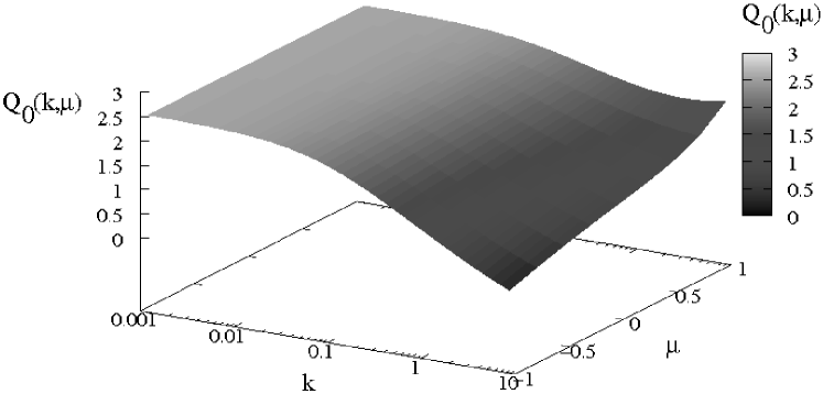
Figure 9: The zeroth order downstream eigenfunction for shock speed $u_{-}=.3$. Along the $x$-axis we have plotted the logarithm of $k_{+}$ while along the $y$-axis we have $\mu_{+}$. Up the $z$-axis we have plotted $Q_{0}(k_{+},\mu_{+})$, which also defines the grayscale. Note the anisotropy increases with $k_{+}$.

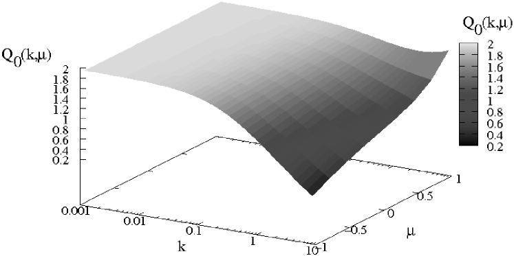
Figure 10: The zeroth order downstream eigenfunction for shock speed $u_{-}=.5$. Along the $x$-axis we have plotted the logarithm of $k_{+}$ while along the $y$-axis we have $\mu_{+}$. Up the $z$-axis we have plotted $Q_{0}(k_{+},\mu_{+})$, which also defines the grayscale. Note the anisotropy increases with $k_{+}$.

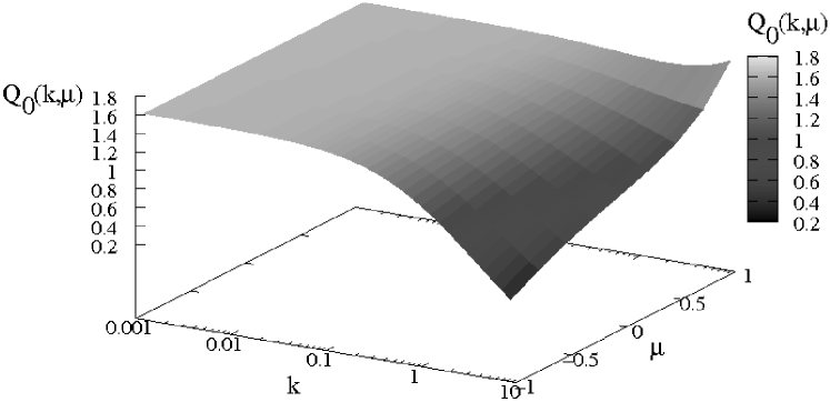
Figure 11: The zeroth order downstream eigenfunction for shock speed $u_{-}=.7$. Along the $x$-axis we have plotted the logarithm of $k_{+}$ while along the $y$-axis we have $\mu_{+}$. Up the $z$-axis we have plotted $Q_{0}(k_{+},\mu_{+})$, which also defines the greyscale. Note the anisotropy increases with $k_{+}$.

Figures 9, 10 and 11 show how anisotropy arises in the zeroth order eigenfunction which is isotropic for $k=0$. Given that $k$ is related to the momentum these figures show that, since this is the dominant eigenfunction, the anisotropy will increase with increasing energy.

3.2 Shock matching conditions

Starting from

$${\hat{W}}(k,\mu,z) =\sum_{i}a_{i}(k)X_{i}(k,z)Q_{i}(k,\mu)$$ (42)

$$=\sum_{i}a_{i}(k)\exp\left(\frac{\Lambda_{i}(k)z}{\Gamma}\right)Q_{i}(k,\mu))$$ (43)

we note that upstream $(z<0)$ we have $a_{i}=0$ for all $i$ such that $\Lambda_{i}\leq 0$ and that downstream $(z>0)$ we have $a_{i}=0$ for all $i$ such that $\Lambda_{i}>0$. The distribution function is continuous at the shock,

$$f_{-}(y_{-},\mu_{-},0)=f_{+}(y_{+},\mu_{+},0)$$ (44)

with $(y_{-},\mu_{-})$ related to $(y_{+},\mu_{+})$ by a Lorentz transformation of velocity $u_{\rm rel}=(u_{-}-u_{+})/(1-u_{-}u_{+})$,

$$y_{-} =\Gamma_{\rm rel}y_{+}(1+u_{\rm rel}\mu_{-}).$$ (45)

In terms of $W$ the matching condition becomes

$$\Gamma_{\rm rel}^{4}(1+u_{\rm rel}\mu_{-})^{4}W_{-}(y_{-},\mu_{-},0) =W_{+}(y_{+},\mu_{+},0)$$ (46)

and we now need to express this in terms of ${\hat{W}}$, the Laplace transform with respect to $y$. Taking $k_{-}y_{-}=k_{+}y_{+}$, multiplying the matching condition for $W$ by $\exp(-k_{+}y_{+})$ and integrating over $y_{+}$ gives

$$\Gamma_{\rm rel}^{3}(1+u_{\rm rel}\mu_{-})^{3}{\hat{W}}_{-}(k_{-},\mu_{-},0)={\hat{W}}_{+}(k_{+},\mu_{+},0).$$ (47)

Guided by the discussion for the nonrelativistic case, we use the expansion

$${\hat{W}}^{\pm}=\sum_{i}b^{\pm}_{i}k_{\pm}^{-s+3}Q^{\pm}_{i}(k_{\pm},\mu_{\pm})$$ (48)

so that the matching condition for the Laplace transformed spectrum at the shock reduces to

$$\Gamma_{\rm rel}^{s}(1+u_{\rm rel}\mu_{-})^{s}\sum_{i}b_{i}^{-}(k_{-})Q_{i}^{-}(k_{-},\mu_{-})=$$

$$\sum_{i}b_{i}^{+}(k_{+})Q^{+}_{i}(k_{+},\mu_{+}).$$ (49)

In order to solve for the particle spectrum, we multiply by $(u_{+}+\mu_{+}){Q}^{+}_{j}(k_{+},\mu_{+})\;j\geq 0$ and integrate over $\mu_{+}$. Then for a fixed $k_{-}$ we have

$$\sum_{i}b_{i}^{-}(k_{-})\int_{-1}^{1} (1+u_{rel}\mu_{-})^{s}Q_{i}^{-}(k_{-},\mu_{-})\times$$

$$(u_{+}+\mu_{+}){Q}^{+}_{j}(k_{+},\mu_{+})d\mu_{+}=0.$$ (50)

Defining a matrix ${\bf S}$ with elements

$$S^{-}_{i,j}=\int_{-1}^{1}(1+u_{\rm rel}\mu_{-})^{s}Q_{i}^{-}(k_{-},\mu_{-})(u_{+}+\mu_{+}){Q}^{+}_{j}(k_{+},\mu_{+})d\mu_{+}$$ (51)

we need to find the spectral index $s$, such that $\det{\bf S}=0$. The Laplace inversion is then carried out numerically (see Appendix for details). As motivated by the nonrelativistic case, we define the cut-off to be the point at which

$$\left.\frac{d(\ln R)}{d(\ln k)}\right|_{p_{\rm cut}}=-1$$ (52)

where $R=\sum b_{i}Q_{i}$. Figures 12, 13 and 14 plot $d(\ln R)/d(\ln k)$ at the shock against $k$ as measured downstream. The results are summarised in table 2.

Figure 12: Plotted along the $x$-axis we have the logarithm of momentum $k_{+}$ while along the $y$-axis we have $d(\ln R_{+})/d(\ln k_{+})$ for $u_{-}=.3$ and $R_{+}=\sum_{i}b^{+}_{i}(k_{+})Q_{i}^{+}(k_{+},\mu_{+})$. Note the cut-off depends on $\mu_{+}$

Figure 13: Plotted along the $x$-axis we have the logarithm of momentum $k_{+}$ while along the $y$-axis we have $d(\ln R_{+})/d(\ln k_{+})$ for $u_{-}=.5$ and $R_{+}=\sum_{i}b^{+}_{i}(k_{+})Q_{i}^{+}(k_{+},\mu_{+})$. Note the cut-off depends on $\mu_{+}$

Figure 14: Plotted along the $x$-axis we have the logarithm of momentum $k_{+}$ while along the $y$-axis we have $d(\ln R_{+})/d(\ln k_{+})$ for $u_{-}=.7$ and $R_{+}=\sum_{i}b^{+}_{i}(k_{+})Q_{i}^{+}(k_{+},\mu_{+})$. Note the cut-off depends on $\mu_{+}$

$u_{-}$	.3	.5	.7
$u_{+}$	.076	.129	.189
$\Gamma_{\rm rel}$	1.027	1.089	1.23
$p^{\ast}$	.404	1.143	2.26
Non-Rel $p_{\rm cut}$	.621	1.79	3.719
$p_{\rm cut}(\mu_{+}=-1.0)$	.541	1.42	2.566
$p_{\rm cut}(\mu_{+}=-0.5)$	.595	1.71	3.612
$p_{\rm cut}(\mu_{+}=0)$	.64	1.929	4.375
$p_{\rm cut}(\mu_{+}=0.5)$	.682	2.138	5.105
$p_{\rm cut}(\mu_{+}=1)$	.741	2.533	6.773

Table 2: Summary of Cut-Off Momenta

Figures 12, 13 and 14 show how the cut-off momentum becomes increasing anisotropic as the shock speed increases.

Figure 15: The downstream function evaluated at the shock for a shock speed of .3. Along the $x$-axis we have plotted the logarithm of momentum $p_{+}$ while along the $y$-axis we have the logarithm of $W=p^{4}f$.

Figure 16: The downstream function evaluated at the shock for a shock speed of .5. Along the $x$-axis we have plotted the logarithm of momentum $p_{+}$ while along the $y$-axis we have the logarithm of $W=p^{4}f$.

The distribution can be fitted approximately by

$$f\approx p^{-s}\exp\left(-\left(\frac{p}{\sqrt{\Gamma_{\rm rel}}p_{\rm cut}(\mu_{+})}\right)^{\beta}\right)$$ (53)

where $\beta$ is typically 2. However it is difficult justify the use of the factor $\sqrt{\Gamma_{\rm rel}}$ in general as our results are only for mildly relativistic shocks. This fit justifies our definition of $p_{\rm cut}$ instead of using the equilibrium momentum $p^{\ast}$. Figure 17 illustrates this approximation for a .7c shock. $\beta$ seems to be pitch angle dependent varying between 1.75 and 2.2, but typically 2. In fact for the .3c and .5c shock cases $\beta$ showed much less variation about 2.

Figure 17: The downstream function evaluated at the shock for a shock speed of .7. Along the $x$-axis we have plotted the logarithm of momentum $p_{+}$ while along the $y$-axis we have the logarithm of $W=p^{4}f$. The lines are data while the points are the best fit described in the text.

For the shock speeds we have chosen, with the Juttner-Synge equation of state, the spectral indices in the absence of losses are close to $4$.

Figures 15,  16 and  17 illustrated a feature that was not present in the non-relativistic case. The pitch angle dependence of the cut-off momentum leads to a difference in the isotropy levels between particles above and below some critical momentum $p_{\rm aniso}$. Indeed there is a clear pattern of greater levels of anisotropy at high energies as the shock speed increases, despite the fact that the results presented here are only for mildly relativistic shocks.

3.3 The Spatially Integrated Distribution

While the method we follow in this paper finds the upstream particle distribution directly, it is easy to find the downstream distribution by using the matching condition, as discussed in the previous section. The downstream distribution is, in many respects, more important physically as it will be responsible form most of the spatial integrated emission. As it can be difficult to spatially resolve observational data from non-thermal emitters, we must consider the emission from an extended region of space. Our eigenfunction expansion allows us to do this quite easily. The spatially averaged distribution from a downstream region $[z_{0},z_{1}]$ in terms of Laplace variables is

$$R_{[z_{0},z_{1}]}(k_{+},\mu_{+})=\sum_{i\leq 0}a_{i}(k)\left(\exp\left(\frac{\Lambda^{+}_{i}(k_{+})z_{1}}{\Gamma_{+}}\right)\right.$$

$$-\left.\exp\left(\frac{\Lambda^{+}_{i}(k_{+})z_{0}}{\Gamma_{+}}\right)\right)\frac{\Gamma_{+}Q^{+}_{i}(\mu_{+},k_{+})}{\Lambda^{+}_{i}(k_{+})}.$$ (54)

In the case of a source which is completely spatially unresolved this reduces to

$$R_{[0,\infty]}(k_{+},\mu_{+})=-\Gamma_{+}\sum_{i\leq 0}a_{i}(k)\frac{Q^{+}_{i}(\mu_{+},k_{+})}{\Lambda^{+}_{i}(k_{+})}.$$ (55)

Of course the optical depth of the emitting region will also have an effect on the spectrum of unresolved sources by reducing $z_{1}$.

Figure 18: The downstream function integrated for a shock speed of .3 between $z^{\prime}=0$ and $z^{\prime}=100$ where $z^{\prime}=Dz/\Gamma_{+}$. Along the $x$-axis we have plotted the logarithm of momentum $p_{+}$ while along the $y$-axis we have the logarithm of $W=p^{4}f$.

Figure 19: The downstream function integrated for a shock speed of .5 between $z^{\prime}=0$ and $z^{\prime}=100$ where $z^{\prime}=Dz/\Gamma_{+}$. Along the $x$-axis we have plotted the logarithm of momentum $p_{+}$ while along the $y$-axis we have the logarithm of $W=p^{4}f$.

Figure 20: The downstream function integrated for a shock speed of .7 between $z^{\prime}=0$ and $z^{\prime}=100$ where $z^{\prime}=Dz/\Gamma_{+}$. Along the $x$-axis we have plotted the logarithm of momentum $p_{+}$ while along the $y$-axis we have the logarithm of $W=p^{4}f$.

Figure 21: Synchrotron emission from the particle distribution shown in 18 measured in the downstream medium. In plotting our $\mu=\pm 1$ we used $\mu=\pm.9999$ as there is no emission from an ordered field along $\mu=\pm 1$.

Figure 22: Synchrotron emission from the particle distribution shown in 19 measured in the downstream medium. In plotting our $\mu=\pm 1$ we used $\mu=\pm.9999$ as there is no emission from an ordered field along $\mu=\pm 1$.

Figure 23: Synchrotron emission from the particle distribution shown in 20 measured in the downstream medium. In plotting our $\mu=\pm 1$ we used $\mu=\pm.9999$ as there is no emission from an ordered field along $\mu=\pm 1$.

Using the same numerical Laplace inversion as in the non-relativistic case we have calculated the distribution functions and synchrotron emission. Figures 18, 19 and 20 show the spatially integrated distribution functions for a finite emission region. Now there are there features: a momentum break, $p_{\rm b}$, due to spatial effect; an anisotropic break, $p_{\rm aniso}$, due to relativistic effects; and a cut-off, $p_{\rm cut}$, due to energy losses. Given that the magnetic field is constant throughout this region it is trivial to produce the associated synchrotron emission plots of figures 21, 22 and 23. It should be noted that in the emission plots $I_{\nu}$ is measured in the downstream frame, but since $I_{\nu}/\nu^{3}$ is a Lorentz invariant the transformation is trivial. The synchrotron emission also includes the same three features we observed in the particle distribution; namely a break frequency beyond which the effect of synchrotron cooling becomes important, a frequency at which pitch-angle or anisotropic effects play a role and an upper cut-off beyond which there is virtually no emission.

4 Discussion

Particle acceleration and self-consistent synchrotron radiation have been considered previously by Kirk et al. (1998) using a zonal model. They were successful in explaining the radio to X-ray spectrum of Mkn 501. However such zonal models typically depend on isotropic particle distributions. We have shown, however, that for particles near the high energy cut-off this is not true even for mildly relativistic flows. The computational resources available restricted our results to be below .7c. However even for the mildly relativistic shock velocities we see a clear pattern of high energy anisotropy emerging resulting in synchrotron emission which is also anisotropic. This could be extremely important in the modelling of the inverse Compton hump in $\gamma$-rays observed in TeV Blazars (Aharonian et al., 2006). As a second implication of the particle anisotropy, in the presence of losses, the idealised situation, of a two sided strongly polarised identical jet system can be considered. Each jet contains only forward external shocks, and the jet which is directed towards the observer is inclined at an angle $\theta=\cos^{-1}(-\mu)$ to the line of sight (magnetic field direction same as that of shock). Then we will observe the emission from particles in the jet directed towards us which have pitch angle $\mu$ and from particles in the jet directed away from us which have pitch angle $-\mu$. While at low energies the only difference between the observed emission of the two jets will be as a result of the effects of beaming, at energies near the synchrotron cut-off the details of the acceleration mechanism will amplify this difference, depending on viewing angle.

Although the work in this paper is limited to an idealised form of diffusion, and mildly relativistic shocks, it illustrates previous unexamined features which could be important in the modelling of relativistic, $\gamma$-ray sources such as microquasars, blazars and GRBs. We have parameterised the exponential shape of the distribution cut-off and identified new pitch angle dependent features between break and cut-off frequencies. Further work is needed to examine both momentum dependent scattering and high Lorentz factor flows.

Appendix A Inverse Laplace Transforms

While Heavens & Meisenheimer (1987) invert the Laplace transform analytically for particular cases here we use numerical methods as we will need to when dealing with relativistic flows.

Formally the inverse Laplace transform is the Bromwich integral, which is a complex integral given by:

$$f(t)=\mathcal{L}^{-1}\left[F(s)\right]=\frac{1}{2\pi i}\int_{\gamma-i\infty}^{\gamma+i\infty}e^{st}F(s)\;ds$$ (56)

where $\gamma$ is to the right of every singularity of $F(s)$. If the singularity of $F(s)$ all ly in the left half of the complex plane $\gamma$ can be set to $0$ and this reduces to the inverse Fourier transform, which is easy to do. However for complicated or numerical Laplace functions the Bromwich integral is extremely difficult to solve. The four main numerical inversion techniques are Fourier Series Expansion, Talbot’s method, Weeks method and methods based on the Post-Widder formula. However some of these methods converge rather slowly and a lot of work has gone into creating acceleration methods. Numerical Laplace inversion is a area of active research and the choice of inversion technique is as much an art as a science at the moment. In this paper the Post-Widder based method was chosen and only these methods shall by described below. Let $F(s)$ be the Laplace transform of $f(t)$ then Widder (1932) showed that $f_{n}(t)\rightarrow f(t)$ where

$$f_{n}(t)=\frac{(-1)^{n}}{n!}\left(\frac{n+1}{t}\right)^{n+1}\hat{f}^{(n)}((n+1)/t).$$ (57)

The advantage of this method in our case in that we see that the Laplace transform of the solution times the Laplace coordinate is the zeroth order approximation to the actual solution.

$$W_{0}(y)=\left(\frac{1}{y}\right)\hat{W}(1/y)\Rightarrow W_{0}(p)=p\hat{W}(p).$$

When dealing with numerical results however it is easier to use the Gaver-Stehfest algorithm (Abate & Valkó, 2004). It is an algorithm based on the Post-Widder method with the Gaver approximants, $\{f_{n}(t):n\geq 0\}$, defined as

$$f_{n}(t)\equiv\frac{(n+1)\ln(2)}{t}\binom{2(n+1)}{n+1}\times$$

$$\sum_{k=0}^{n+1}\binom{n+1}{k}\hat{f}\left((n+1+k)\ln(2)/t\right).$$ (58)

However the convergence for both these methods is slow. A test of methods for accelerating this convergence can be found in Valkó & Abate (2004) and two are found to be quite good: the non-linear Wynn’s Rho Algorithm and the linear Salzer summation. Again a choice has to be made and here we present only Salzer summation: $f(t,M)\rightarrow f(t)$ where

$$f(t,M)=\sum_{k=1}^{M}W_{k}f_{k-1}(t)$$ (59)

and

$$W_{k}=(-1)^{k+M}\frac{k^{M}}{M!}\binom{M}{k}.$$ (60)

The Post-Widder method based on differentiation was implemented in Maple with the Salzer acceleration. It was used to produce the results in the non-relativistic limit as we have an analytic form of the Laplace function to work with. The Salzer accelerated Gaver-Stehfest algorithm was implemented in C/C++ code for use with the numerical output from the relativistic approach discussed above.

Appendix B Deriving the eigensystem differential equations

The solutions, $Q_{i}$, to equation 36

$$\frac{\partial}{\partial\mu}\left(D(\mu)(1-\mu^{2})\frac{\partial Q_{i}}{\partial\mu}\right)-x\lambda g(\mu)Q_{i}=\Lambda_{i}(u+\mu)Q_{i}$$ (61)

for real $x$, are orthogonal, with weight $u+\mu$ and have real, distinct eigenvalues $\Lambda_{i}$ (Boas, 1983). Taking the derivative of this equation with respect to $x$ gives

$$\frac{\partial}{\partial\mu}\left(D(\mu)(1-\mu^{2})\frac{\partial}{\partial\mu}\frac{\partial Q_{i}}{\partial x}\right)-x\lambda g(\mu)\frac{\partial Q_{i}}{\partial x}$$

$$=\Lambda_{i}(u+\mu)\frac{\partial Q_{i}}{\partial x}+\left(\frac{d\Lambda_{i}}{dx}(u+\mu)+\lambda g(\mu)\right)Q_{i}.$$ (62)

Since solution to Sturm Liouville equations form an orthogonal basis, we can write

$$\frac{\partial Q_{i}}{\partial x}=\sum_{m}q_{m}Q_{m}$$ (63)

which gives

$$\sum_{m}q_{m}\frac{\partial}{\partial\mu}\left(D(\mu)(1-\mu^{2})\frac{\partial}{\partial\mu}Q_{m}\right)-\sum_{m}q_{m}x\lambda g(\mu)Q_{m}$$

$$=\sum_{m}q_{m}\Lambda_{m}(u+\mu)Q_{m}$$

$$=\sum_{m}q_{m}\Lambda_{i}(u+\mu)Q_{m}+\left(\frac{d\Lambda_{i}}{dx}(u+\mu)+\lambda g(\mu)\right)Q_{i}.$$ (64)

Multiplying by $Q_{j}^{*}$ and integrating over $\mu$ gives

$$\sum_{m}q_{m}(\Lambda_{m}-\Lambda_{i})\langle Q_{j},Q_{m}\rangle$$

$$=\frac{d\Lambda_{i}}{dx}\langle Q_{j},Q_{i}\rangle+\lambda\int_{-1}^{1}g(\mu)Q_{i}Q_{j}^{*}\;d\mu.$$ (65)

Taking $j=i$ implies equation 41 and $j\neq i$ implies equation 40.

References

- Abate & Valkó (2004) Abate J., Valkó P.P., 2004, International Journal for Numerical Methods in Engineering, 60, 979
- Aharonian et al. (2006) Aharonian F., et al. 2006, A&A, 455, 461
- Boas (1983) Boas M.L., 1983, Mathematical Methods in the Physical Sciences, Ed., John Wiley & Sons
- Heavens & Drury (1988) Heavens A.F., Drury L.O’C., 1988, MNRAS, 235, 997
- Heavens & Meisenheimer (1987) Heavens A.F., Meisenheimer K., 1987, MNRAS, 225, 335
- Kirk et al. (2000) Kirk J.G., Guthmann A.W., Gallant Y.A., Achterberg A., 2000, ApJ, 542, 235
- Kirk et al. (1998) Kirk, J. G., Rieger, F. M., & Mastichiadis, A., 1998, A&A, 333, 452
- Kirk & Schneider (1987) Kirk J.G., Schneider P., 1987, ApJ, 323, L87
- Rybicki & Lightman (1986) Rybicki, G. B., & Lightman, A. P. 1986, Radiative Processes in Astrophysics.
- Webb et al. (1984) Webb G.M., Drury L.O’C., Biermann P., 1983, A&A, 137, 185
- Valkó & Abate (2004) Valkó P.P., Abate J., 2004, Computers and Mathematics with Application, 48, 629
- Widder (1932) Widder D. V., 1932, PNAS, 18, 181