IFT-UAM/CSIC-07-14

CERN-PH-TH/2007-063

Supersymmetry breaking metastable vacua
in runaway quiver gauge theories
I. García-Etxebarria, F. Saad, A.M.Uranga
PH-TH Division, CERN CH-1211 Geneva 23, Switzerland
and
Instituto de Física Teórica C-XVI,
Universidad Autónoma de Madrid, Cantoblanco, 28049 Madrid, Spain
Abstract

In this paper we consider quiver gauge theories with fractional branes whose infrared dynamics removes the classical supersymmetric vacua (DSB branes). We show that addition of flavors to these theories (via additional non-compact branes) leads to local meta-stable supersymmetry breaking minima, closely related to those of SQCD with massive flavors. We simplify the study of the one-loop lifting of the accidental classical flat directions by direct computation of the pseudomoduli masses via Feynman diagrams. This new approach allows to obtain analytic results for all these theories. This work extends the results for the $dP_{1}$ theory in hep-th/0607218. The new approach allows to generalize the computation to general examples of DSB branes, and for arbitrary values of the superpotential couplings.

1 Introduction

Systems of D-branes at singularities provide a very interesting setup to realize and study diverse non-perturbative gauge dynamics phenomena in string theory. In the context of $\mathcal{N}=1$ supersymmetric gauge field theories, systems of D3-branes at Calabi-Yau singularities lead to interesting families of tractable 4d strongly coupled conformal field theories, which extend the AdS/CFT correspondence [1, 2, 3] to theories with reduced (super)symmetry [4, 5, 6] and enable non-trivial precision tests of the correspondence (see for instance [7, 8]). Addition of fractional branes leads to families of non-conformal gauge theories, with intricate RG flows involving cascades of Seiberg dualities [9, 10, 11, 12, 13], and strong dynamics effects in the infrared.

For instance, fractional branes associated to complex deformations of the singular geometry (denoted deformation fractional branes in [12]), correspond to supersymmetric confinement of one or several gauge factors in the gauge theory [9, 12]. The generic case of fractional branes associated to obstructed complex deformations (denoted DSB branes in [12]), corresponds to gauge theories developing a non-perturbative Affleck-Dine-Seiberg superpotential, which removes the classical supersymmetric vacua [14, 15, 16]. As shown in [15] (see also [17, 18]), assuming canonical Kahler potential leads to a runaway potential for the theory, along a baryonic direction. A natural suggestion to stop this runaway has been proposed for the particular example of the $dP_{1}$ theory (the theory on fractional branes at the complex cone over $dP_{1}$) in [19]. It was shown that, upon the addition of D7-branes to the configuration (which introduce massive flavors), the theory develops a meta-stable minimum (closely related to the Intriligator-Seiberg-Shih (ISS) model [20]), parametrically long-lived against decay to the runaway regime (see [21] for an alternative suggestion to stop the runaway, in compact models).

In this paper we show that the appearance of meta-stable minima in gauge theories on DSB fractional branes, in the presence of additional massless flavors, is much more general (and possibly valid in full generality). We use the tools of [15] to introduce D7-branes on general toric singularities, and give masses to the corresponding flavors. Since quiver gauge theories are rather involved, we develop new techniques to efficiently analyze the one-loop stability of the meta-stable minima, via the direct computation of Feynman diagrams. These tools can be used to argue that the results plausibly hold for general systems of DSB fractional branes at toric singularities. It is very satisfactory to verify the correspondence between the existence of meta-stable vacua and the geometric property of having obstructed complex deformations.

The present work thus enlarges the class of string models realizing dynamical supersymmetry breaking in meta-stable vacua (see [22, 23, 24, 25, 26] for other proposed realizations, and [27, 28, 29] for models of dynamical supersymmetry breaking in orientifold theories). Although we will not discuss it in the present paper, these results can be applied to the construction of models of gauge mediation in string theory as in [30] (based on the additional tools in [31]), in analogy with [32]. This is another motivation for the present work.

The paper is organized as follows. In Section 2 we review the ISS model, evaluating one-loop pseudomoduli masses directly in terms of Feynman diagrams. In Section 3 we study the theory of DSB branes at the $dP_{1}$ and $dP_{2}$ singularities upon the addition of flavors, and we find that metastable vacua exist for these theories. In Section 4 we extend this analysis to the general case of DSB branes at toric singularities with massive flavors, and we illustrate the results by showing the existence of metastable vacua for DSB branes at some well known families of toric singularities. Finally, the Appendix provides some technical details that we have omitted from the main text in order to improve the legibility.

2 The ISS model revisited

In this Section we review the ISS meta-stable minima in SQCD, and propose that the analysis of the relevant piece of the one-loop potential (the quadratic terms around the maximal symmetry point) is most simply carried out by direct evaluation of Feynman diagrams. This new tool will be most useful in the study of the more involved examples of quiver gauge theories.

2.1 The ISS metastable minimum

The ISS model [20] (see also [33] for a review of these and other models) is given by ${\cal N}=1$ $SU(N_{c})$ theory with $N_{f}$ flavors, with small masses

$$W_{\textrm{electric}}=m{\rm Tr\,}\phi\tilde{\phi},$$ (2.1)

where $\phi$ and $\tilde{\phi}$ are the quarks of the theory. The number of colors and flavors are chosen so as to be in the free magnetic phase:

$$N_{c}+1\leq N_{f}<\frac{3}{2}N_{c}.$$ (2.2)

This condition guarantees that the Seiberg dual is infrared free. This Seiberg dual is the $SU(N)$ theory (with $N=N_{f}-N_{c}$) with $N_{f}$ flavors of dual quarks $q$ and $\tilde{q}$ and the meson $M$. The dual superpotential is given by rewriting (2.1) in terms of the mesons and adding the usual coupling between the meson and the dual quarks:

$$W_{\textrm{magnetic}}\,=\,h\,({\rm Tr\,}\tilde{q}Mq-\mu^{2}{\rm Tr\,}M),$$ (2.3)

where $h$ and $\mu$ can be expressed in terms of the parameters $m$ and $\Lambda$, and some (unknown) information about the dual Kähler metric. It was also argued in [20] that it is possible to study the supersymmetry breaking minimum in the origin of (dual) field space without taking into account the gauge dynamics (their main effect in this discussion consists of restoring supersymmetry dynamically far in field space). In the following we will assume that this is always the case, and we will forget completely about the gauge dynamics of the dual.

Once we forget about gauge dynamics, studying the vacua of the dual theory becomes a matter of solving the F-term equations coming from the superpotential (2.3). The mesonic F-term equation reads:

$$-\overline{F}_{M_{ij}}=h\tilde{q}^{i}\cdot q^{j}-h\mu^{2}\delta^{ij}=0,$$ (2.4)

where $i$ and $j$ are flavor indices and the dot denotes color contraction. This has no solution, since the identity matrix $\delta^{ij}$ has rank $N_{f}$ while $\tilde{q}^{i}\cdot q^{j}$ has rank $N=N_{f}-N_{c}$. Thus this theory breaks supersymmetry spontaneously at tree level. This mechanism for F-term supersymmetry breaking is called the rank condition.

The classical scalar potential has a continuous set of minima, but the one-loop potential lifts all of the non-Goldstone directions, which are usually called pseudomoduli. The usual approach to study the one-loop stabilization is the computation of the complete one-loop effective potential over all pseudomoduli space via the Coleman-Weinberg formula [34]:

$$V=\frac{1}{64\pi^{2}}{\rm Tr\,}\left({\cal M}_{B}^{4}\log\frac{{\cal M}_{B}^{2}}{\Lambda^{2}}-{\cal M}_{F}^{4}\log\frac{{\cal M}_{F}^{2}}{\Lambda^{2}}\right).$$ (2.5)

This approach has the advantage that it allows the determination of the one-loop minimum, without a priori information about its location, and moreover it provides the full potential around it, including higher terms. However, it has the disadvantage of requiring the diagonalization of the mass matrix, which very often does not admit a closed expression, e.g. for the theories we are interested in.

In fact, we would like to point out that to determine the existence of a meta-stable minimum there exists a computationally much simpler approach. In our situation, we have a good ansatz for the location of the one-loop minimum, and are interested just in the one-loop pseudomoduli masses around such point. This information can be directly obtained by computing the one-loop masses via the relevant Feynman diagrams. This technique is extremely economical, and provides results in closed form in full generality, e.g. for general values of the couplings, etc. The correctness of the original ansatz for the vacuum can eventually be confirmed by the results of the computation (namely positive one-loop squared masses, and negligible tadpoles for the classically massive fields ).

Hence, our strategy to study the one-loop stabilization in this paper is as follows:

• First we choose an ansatz for the classical minimum to become the one-loop vacuum. It is natural to propose a point of maximal enhanced symmetry (in particular, close to the origin in the space of vevs for $M$ there exist and R-symmetry, whose breaking by gauge interactions (via anomalies) is negligible in that region). Hence the natural candidate for the one-loop minimum is

  $$q=\tilde{q}^{\mathrm{T}}=\left(\begin{array}[]{c}\mu\\ 0\end{array}\right),$$ (2.6)

  with the rest of the fields set to 0. This initial ansatz for the one-loop minimum is eventually confirmed by the positive square masses at one-loop resulting from the computations described below. In our more general discussion of meta-stable minima in runaway quiver gauge theories, our ansatz for the one-loop minimum is a direct generalization of the above (and is similarly eventually confirmed by the one-loop mass computation).

• Then we expand the field linearly around this vacuum, and identify the set of classically massless fields. We refer to these as pseudomoduli (with some abuse of language, since there could be massless fields which are not classically flat directions due to higher potential terms)

• As a final step we compute one-loop masses for these pseudomoduli by evaluating their two-point functions via conventional Feynman diagrams, as explained in more detail in appendix A.1 and illustrated below in several examples.

The ISS model is a simple example where this technique can be illustrated. Considering the above ansatz for the vacuum, we expand the fields around this point as:

$$q=\left(\begin{array}[]{c}\mu+\frac{1}{\sqrt{2}}(\xi_{+}+\xi_{-})\\ \frac{1}{\sqrt{2}}(\rho_{+}+\rho_{-})\end{array}\right),\qquad\tilde{q}^{\mathrm{T}}=\left(\begin{array}[]{c}\mu+\frac{1}{\sqrt{2}}(\xi_{+}-\xi_{-})\\ \frac{1}{\sqrt{2}}(\rho_{+}-\rho_{-})\end{array}\right),\qquad M=\left(\begin{array}[]{cc}Y&Z\\ \tilde{Z}^{\mathrm{T}}&\Phi\end{array}\right),$$ (2.7)

where we have taken linear combinations of the fields in such a way that the bosonic mass matrix is diagonal. This will also be convenient in section 2.2, where we discuss the Goldstone bosons in greater detail.

We now expand the superpotential (2.3) to get

$$W = \sqrt{2}\mu\xi_{+}Y+\frac{1}{\sqrt{2}}\mu Z\rho_{+}+\frac{1}{\sqrt{2}}\mu Z\rho_{-}+\frac{1}{\sqrt{2}}\mu\rho_{+}\tilde{Z}-\frac{1}{\sqrt{2}}\mu\rho_{-}\tilde{Z}$$ (2.8)

$$+\frac{1}{2}\rho_{+}^{2}\Phi-\frac{1}{2}\rho_{-}^{2}\Phi-\mu^{2}\Phi+\ldots,$$

where we have not displayed terms of order three or higher in the fluctuations, unless they contain $\Phi$, since they are irrelevant for the one loop computation we will perform. Note also that we have set $h=1$ and we have removed the trace (the matricial structure is easy to restore later on, here we just set $N_{f}=2$ for simplicity). The massless bosonic fluctuations are given by ${\rm Re}\,\rho_{+}$, ${\rm Im}\,\rho_{-}$, $\Phi$ and $\xi_{-}$. The first two together with ${\rm Im}\,\xi_{-}$ are Goldstone bosons, as explained in section 2.2. Thus the pseudomoduli we are interested in are given by $\Phi$ and ${\rm Re}\,\xi_{-}$. Let us focus on $\Phi$ (the case of ${\rm Re}\,\xi_{-}$ admits a similar discussion). In this case the relevant terms in the superpotential simplify further, and just the following superpotential contributes:

$$W = \mu Z\frac{1}{\sqrt{2}}(\rho_{+}+\rho_{-})+\mu\tilde{Z}\frac{1}{\sqrt{2}}(\rho_{+}-\rho_{-})+\frac{1}{2}\rho_{+}^{2}\Phi-\frac{1}{2}\rho_{-}^{2}\Phi-\mu^{2}\Phi+\ldots,$$

which we recognize, up to a field redefinition, as the symmetric model of appendix A.2. We can thus directly read the result

$$\delta m^{2}_{\Phi}=\frac{|h|^{4}\mu^{2}}{8\pi^{2}}(\log 4-1).$$ (2.9)

This matches the value given in [20], which was found using the Coleman-Weinberg potential.

2.2 The Goldstone bosons

One aspect of our technique that merits some additional explanation concerns the Goldstone bosons. The one-loop computation of the masses for the fluctuations associated to the symmetries broken by the vacuum, using just the interactions described in appendix A.1, leads to a non-vanishing result. This puzzle is however easily solved by realizing that certain (classically massive) fields have a one-loop tadpole. This leads to a new contribution to the one-loop Goldstone two-point amplitude, given by the diagram in Figure 1. Adding this contribution the total one-loop mass for the Goldstone bosons is indeed vanishing, as expected. This tadpole does not affect the computation of the one-loop pseudomoduli masses (except for ${\rm Re}\,\xi_{+}$, but its mass remains positive) as it is straightforward to check.

Figure 1: Schematic tadpole contribution to the ${\rm Im}\,\xi_{-}$ two point function. Both bosons and fermions run in the loop.

The structure of this cancellation can be understood by using the derivation of the Goldstone theorem for the 1PI effective potential, as we now discuss. The proof can be found in slightly more detail, together with other proofs, in [35]. Let us denote by $V$ the 1PI effective potential. Invariance of the action under a given symmetry implies that

$$\frac{\delta V}{\delta\phi_{i}}\Delta\phi_{i}=0,$$ (2.10)

where we denote by $\Delta\phi_{i}$ the variation of the field $\phi_{i}$ under the symmetry, which will in general be a function of all the fields in the theory. Taking the derivative of this equation with respect to some other field $\phi_{k}$

$$\frac{\delta^{2}V}{\delta\phi_{i}\delta\phi_{k}}\Delta\phi_{i}+\frac{\delta V}{\delta\phi_{i}}\cdot\frac{\delta\Delta\phi_{i}}{\delta\phi_{k}}=0.$$ (2.11)

Let us consider how this applies to our case. At tree level, there is no tadpole and the above equation (truncated at tree level) states that for each symmetry generator broken by the vacuum, the value of $\Delta\phi_{i}$ gives a nonvanishing eigenvector of the mass matrix with zero eigenvalue. This is the classical version of the Goldstone theorem, which allows the identification of the Goldstone bosons of the theory.

For instance, in the ISS model in the previous section (for $N_{f}=2$), there are three global symmetry generators broken at the minimum described around (2.6). The $SU(2)\times U(1)$ symmetry of the potential gets broken down to a $U(1)^{\prime}$, which can be understood as a combination of the original $U(1)$ and the $t_{z}$ generator of $SU(2)$. The Goldstone bosons can be taken to be the ones associated to the three generators of $SU(2)$, and correspond (for $\mu$ real) to ${\rm Im}\,\xi_{-}$, ${\rm Im}\,\rho_{-}$ and ${\rm Re}\,\rho_{+}$, in the parametrization of the fields given by equation (2.7).

Even in the absence of tree-level tadpoles, there could still be a one-loop tadpole. When this happens, there should also be a non-trivial contribution to the mass term for the Goldstone bosons in the one-loop 1PI potential, related to the tadpole by the one-loop version of (2.11). This relation guarantees that the mass term in the physical (i.e. Wilsonian) effective potential, which includes the 1PI contribution, plus those of the diagram in Figure 1, vanishes, as we described above.

In fact, in the ISS example, there is a non-vanishing one-loop tadpole for the real part of $\xi_{+}$ (and no tadpole for other fields). The calculation of the tadpole at one loop is straightforward, and we will only present here the result

$$i{\cal M}=\frac{-i|h|^{4}\mu^{3}}{(4\pi)^{2}}(2\log 2).$$ (2.12)

The 1PI one-loop contribution to the Goldstone boson mass is also simple to calculate, giving the result

$$i{\cal M}=\frac{-i|h|^{4}\mu^{2}}{(4\pi)^{2}}(\log 2).$$ (2.13)

Using the variations of the relevant fields under the symmetry generator, e.g. for $t_{z}$,

$$\Delta{\rm Re}\,\xi_{+} = -{\rm Im}\,\xi_{-}$$ (2.14)

$$\Delta{\rm Im}\,\xi_{-} = {\rm Re}\,\xi_{+}+2\mu.$$ (2.15)

we find that the (2.11) is satisfied at one-loop.

$$\left\langle\frac{\delta^{2}V}{\delta\phi_{i}\delta\phi_{k}}\Delta\phi_{i}+\frac{\delta V}{\delta\phi_{i}}\cdot\frac{\delta\Delta\phi_{i}}{\delta\phi_{k}}\right\rangle=m^{2}_{{\rm Im}\,\xi_{-}}\cdot 2\mu+({\rm Re}\,\xi_{+}\mathrm{tadpole})\cdot(-1)=0.$$ (2.16)

A very similar discussion applies to $t_{x}$ and $t_{y}$.

The above discussion of Goldstone bosons can be similarly carried out in all examples of this paper. Hence, it will be enough to carry out the computation of the 1PI diagrams discussed in appendix A.1, and verify that they lead to positive squared masses for all classically massless fields (with Goldstone bosons rendered massless by the additional diagrams involving the tadpole).

3 Meta-stable vacua in quiver gauge theories with DSB branes

In this section we show the existence of a meta-stable vacuum in a few examples of gauge theories on DSB branes, upon the addition of massive flavors. As already discussed in [19], the choice of fractional branes of DSB kind is crucial in the result. The reason is that in order to have the ISS structure, and in particular supersymmetry breaking by the rank condition, one needs a node such that its Seiberg dual satisfies $N_{f}>N$, with $N=N_{f}-N_{c}$ with $N_{c}$, $N_{f}$ the number of colors, flavors of that gauge factor. Denoting $N_{f,0}$, $N_{f,1}$ the number of massless and massive flavors (namely flavors arising from bi-fundamentals of the original D3-brane quiver, or introduced by the D7-branes), the condition is equivalent to $N_{f,0}<N_{c}$. This is precisely the condition that an ADS superpotential is generated, and is the prototypical behavior of DSB branes [14, 15, 16, 18].

Another important general comment, also discussed in [19], is that theories on DSB branes generically contain one or more chiral multiplets which do not appear in the superpotential. Being decoupled, such fields remain as accidental flat directions at one-loop, so that the one-loop minimum is not isolated. The proper treatment of these flat directions is beyond the reach of present tools, so they remain an open question. However, it is plausible that they do not induce a runaway behavior to infinity, since they parametrize a direction orthogonal to the fields parametrizing the runaway of DSB fractional branes.

3.1 The complex cone over $dP_{1}$

In this section we describe the most familiar example of quiver gauge theory with DSB fractional branes, the $dP_{1}$ theory. In this theory, a non-perturbative superpotential removes the classical supersymmetric vacua [14, 15, 16]. Assuming canonical Kähler potential the theory has a runaway behavior [15, 17]. In this section, we revisit with our techniques the result in [19] that the addition of massive flavors can induce the appearance of meta-stable supersymmetry breaking minima, long-lived against tunneling to the runaway regime. As we show in coming sections, this behavior is prototypical and extends to many other theories with DSB fractional branes. The example is also representative of the computations for a general quiver coming from a brane at a toric singularity, and illustrates the usefulness of the direct Feynman diagram evaluation of one-loop masses.

Consider the $dP_{1}$ theory, realized on a set of $M$ fractional D3-branes at the complex cone over $dP_{1}$. In order to introduce additional flavors, we introduce sets of $N_{f,1}$ D7-branes wrapping non-compact 4-cycles on the geometry and passing through the singular point. We refer the reader to [19], and also to later sections, for more details on the construction of the theory, and in particular on the introduction of the D7-branes. Its quiver is shown in Figure 2, and its superpotential is

$$W = \lambda(X_{23}X_{31}Y_{12}-X_{23}Y_{31}X_{12})$$ (3.1)

$$+ \lambda^{\prime}(Q_{3i}{\tilde{Q}}_{i2}X_{23}+Q_{2j}{\tilde{Q}}_{j1}X_{12}+Q_{1k}{\tilde{Q}}_{k3}X_{31})$$

$$+ m_{3}Q_{3i}{\tilde{Q}}_{k3}\delta_{ik}+m_{2}Q_{2j}{\tilde{Q}}_{i2}\delta_{ji}+m_{1}Q_{1k}{\tilde{Q}}_{j1}\delta_{kj},$$

where the subindices denote the groups under which the field is charged. The first line is the superpotential of the theory of fractional brane, the second line describes 77-73-37 couplings between the flavor branes and the fractional brane, and the last line gives the flavor masses. Note that there is a massless field, denoted $Z_{12}$ in [19], that does not appear in the superpotential. This is one of the decoupled fields mentioned above, and we leave its treatment as an open question.

\psfrag{3i}{$Q_{3i}$}\psfrag{i2}{${\tilde{Q}}_{i2}$}\psfrag{2j}{$Q_{2j}$}\psfrag{j1}{${\tilde{Q}}_{j1}$}\psfrag{1k}{$Q_{1k}$}\psfrag{k3}{${\tilde{Q}}_{k3}$}\includegraphics[scale={0.70}]{extd3d7.eps}

Figure 2: Extended quiver diagram for a $dP_{1}$ theory with flavors, from [19].

We are interested in gauge factors in the free magnetic phase. This is the case for the $SU(3M)$ gauge factor in the regime

$$M+1\leq N_{f,1}<\frac{5}{2}M.$$ (3.2)

To apply Seiberg duality on node 3, we introduce the dual mesons:

$$\begin{array}[]{rlcrl}M_{21}&=\,{1\over\Lambda}X_{23}X_{31}&\quad;&N_{k1}&=\,{1\over\Lambda}{\tilde{Q}}_{k3}X_{31}\\ M_{21}^{\prime}&=\,{1\over\Lambda}X_{23}Y_{31}&\quad;&N_{k1}^{\prime}&=\,{1\over\Lambda}{\tilde{Q}}_{k3}Y_{31}\\ N_{2i}&=\,{1\over\Lambda}X_{23}Q_{3i}&\quad;&\Phi_{ki}&=\,{1\over\Lambda}{\tilde{Q}}_{k3}Q_{3i}\end{array}$$ (3.3)

and we also replace the electric quarks $Q_{3i}$, ${\tilde{Q}}_{k3}$, $X_{23}$, $X_{31}$, $Y_{31}$ by their magnetic duals ${\tilde{Q}}_{i3}$, $Q_{3k}$, $X_{32}$, $X_{13}$, $Y_{13}$. The magnetic superpotential is given by rewriting the confined fields in terms of the mesons and adding the coupling between the mesons and the dual quarks,

$$W = h\,(\,M_{21}X_{13}X_{32}\,+\,M_{21}^{\prime}Y_{13}X_{32}\,+\,N_{2i}{\tilde{Q}}_{i3}X_{32}$$ (3.4)

$$+ N_{k1}X_{13}Q_{3k}\,+\,N_{k1}^{\prime}Y_{13}Q_{3k}\,+\,\Phi_{ki}{\tilde{Q}}_{i3}Q_{3k}\,)$$

$$+ h\mu_{0}\,(\,M_{21}Y_{12}\,-\,M_{21}^{\prime}X_{12}\,)\,+\,\mu^{\prime}\,Q_{1k}N_{k1}\,+\,\mu^{\prime}\,N_{2i}{\tilde{Q}}_{i2}$$

$$- h\mu^{\,2}{\rm Tr\,}\Phi\,+\,\lambda^{\prime}\,Q_{2j}{\tilde{Q}}_{j1}X_{12}\,+\,m_{2}Q_{2i}{\tilde{Q}}_{i2}\,+\,m_{1}Q_{1i}{\tilde{Q}}_{i1}.$$

This is the theory we want to study. In order to simplify the treatment of this example we will disregard any subleading terms in $m_{i}/\mu^{\prime}$, and effectively integrate out $N_{k1}$ and $N_{2i}$ by substituting them by 0. This is not necessary, and indeed the computations in the next sections are exact. We do it here in order to compare results with [19].

As in the ISS model, this theory breaks supersymmetry via the rank condition. The fields $\tilde{Q}_{i3}$, $Q_{3k}$ and $\Phi_{ki}$ are the analogs of $q$, $\tilde{q}$ and $M$ in the ISS case discussed above. This motivates a vacuum ansatz analogous to (2.6) and the following linear expansion:

$$\begin{array}[]{ccccc}\Phi=\left(\begin{array}[]{cc}\phi_{00}&\phi_{01}\\ \phi_{10}&\phi_{11}\end{array}\right)&;&\tilde{Q}_{i3}=\left(\begin{array}[]{c}\mu e^{\theta}+Q_{3,1}\\ \tilde{Q}_{3,2}\end{array}\right)&;&Q_{3i}^{\mathrm{T}}=\left(\begin{array}[]{c}\mu e^{-\theta}+Q_{3,1}\\ Q_{3,2}\end{array}\right)\\ \tilde{Q}_{k1}=\left(\begin{array}[]{c}\tilde{Q}_{1,1}\\ y\end{array}\right)&;&Q_{2j}=\left(\begin{array}[]{cc}Q_{2,11}&x\\ Q_{2,21}&x^{\prime}\end{array}\right)&;&M_{21}=\left(\begin{array}[]{c}M_{21,1}\\ M_{21,2}\end{array}\right)\\ Y_{13}=\left(Y_{13}\right)&;&X_{12}^{\mathrm{T}}=\left(\begin{array}[]{c}X_{12,1}\\ X_{12,2}\end{array}\right)&;&X_{32}^{\mathrm{T}}=\left(\begin{array}[]{c}X_{32,1}\\ X_{32,2}\end{array}\right)\\ Y_{12}^{\mathrm{T}}=\left(\begin{array}[]{c}Y_{12,1}\\ Y_{12,2}\end{array}\right)&;&N^{\prime}_{k1}=\left(\begin{array}[]{c}N^{\prime}_{k1,1}\\ z\end{array}\right)&;&M^{\prime}_{21}=\frac{\lambda^{\prime}}{h\mu_{0}}\left(\begin{array}[]{c}M^{\prime}_{21,1}\\ M^{\prime}_{21,2}\end{array}\right)\\ &&X_{13}=\left(X_{13}\right).\end{array}$$ (3.5)

Note that we have chosen to introduce the nonlinear expansion in $\theta$ in order to reproduce the results found in the literature in their exact form. Note also that for the sake of clarity we have not been explicit about the ranks of the different matrices. They can be easily worked out (or for this case, looked up in [19]), and we will restrict ourselves to the 2 flavor case where the matrix structure is trivial. As a last remark, we are not being explicit either about the definitions of the different couplings in terms of the electric theory. This can be done easily (and as in the ISS case they involve an unknown coefficient in the Kähler potential), but in any event, the existence of the meta-stable vacua can be established for general values of the coefficients in the superpotential. Hence we skip this more detailed but not very relevant discussion.

The next step consists in expanding the superpotential and identifying the massless fields. We get the following quadratic contributions to the superpotential:

$$W_{\mathrm{mass}} = 2h\mu\phi_{00}\tilde{Q}_{3,1}+h\mu\phi_{01}\tilde{Q}_{3,2}+h\mu\phi_{10}Q_{3,2}$$ (3.6)

$$+ h\mu_{0}M_{21,1}Y_{12,1}+h\mu_{0}M_{21,2}Y_{12,2}-\lambda^{\prime}M^{\prime}_{21,1}X_{12,1}-\lambda^{\prime}M^{\prime}_{21,2}X_{12,2}$$

$$+ h\mu N^{\prime}_{k1,1}Y_{13}-h_{1}\mu\tilde{Q}_{1,1}X_{13}-h_{2}\mu Q_{2,11}X_{32,1}-h_{2}\mu Q_{2,21}X_{32,2}.$$

The fields massless at tree level are $x$, $x^{\prime}$, $y$, $z$, $\phi_{11}$, $\theta$, $Q_{3,2}$ and $\tilde{Q}_{3,2}$. Three of these are Goldstone bosons as described in the previous section. For real $\mu$ they are ${\rm Im}\,\theta$, ${\rm Re}\,(\tilde{Q}_{3,2}+Q_{3,2})$ and ${\rm Im}\,(\tilde{Q}_{3,2}-Q_{3,2})$. We now show that all other classically massless fields get masses at one loop (with positive squared masses).

As a first step towards finding the one-loop correction, notice that the supersymmetry breaking mechanism is extremely similar to the one in the ISS model before, in particular it comes only from the following couplings in the superpotential:

$$W_{\mathrm{rank}}=hQ_{3,2}\tilde{Q}_{3,2}\phi_{11}-h\mu^{2}\phi_{11}+\ldots$$ (3.7)

This breaks the spectrum degeneracy in the multiplets $Q_{3,2}$ and $\tilde{Q}_{3,2}$ at tree level, so we refer to them as the fields with broken supersymmetry.

Let us compute now the correction for the mass of $x$, for example. For the one-loop computation we just need the cubic terms involving one pseudomodulus and at least one of the broken supersymmetry fields, and any quadratic term involving fields present in the previous set of couplings. From the complete expansion one finds the following supersymmetry breaking sector:

$$W_{\mathrm{symm.}}=h\phi_{11}Q_{3,2}\tilde{Q}_{3,2}+h\mu\phi_{01}\tilde{Q}_{3,2}+h\mu\phi_{10}Q_{3,2}-h\mu^{2}\phi_{11}.$$ (3.8)

The only cubic term involving the pseudomodulus $x$ and the broken supersymmetry fields is

$$W_{\mathrm{cubic}}=-h_{2}\,x\,\tilde{Q}_{3,2}X_{32,1},$$ (3.9)

and there is a quadratic term involving the field $X_{32,1}$

$$W_{\mathrm{mass\,coupling}}=-h_{2}\mu Q_{2,11}X_{32,1}.$$ (3.10)

Assembling the three previous equations, the resulting superpotential corresponds to the asymmetric model in appendix A.2, so we can directly obtain the one-loop mass for $x$:

$$\delta m^{2}_{x}=\frac{1}{16\pi^{2}}|h|^{4}\mu^{2}{\cal C}\left(\frac{|h_{2}|^{2}}{|h|^{2}}\right).$$ (3.11)

Proceeding in a similar way, the one-loop masses for $\phi_{11}$, $x^{\prime}$, $y$ and $z$ are:

$$\delta m^{2}_{\phi_{11}} = \frac{1}{8\pi^{2}}|h|^{4}\mu^{2}(\log 4-1)$$

$$\delta m^{2}_{x^{\prime}} = \frac{1}{16\pi^{2}}|h|^{4}\mu^{2}{\cal C}\left(\frac{|h_{2}|^{2}}{|h|^{2}}\right),$$

$$\delta m^{2}_{y} = \frac{1}{16\pi^{2}}|h|^{4}\mu^{2}{\cal C}\left(\frac{|h_{1}|^{2}}{|h|^{2}}\right)$$

$$\delta m^{2}_{z} = \frac{1}{16\pi^{2}}|h|^{4}\mu^{2}(\log 4-1).$$ (3.12)

There is just one pseudomodulus left, ${\rm Re}\,\theta$, which is qualitatively different to the others. With similar reasoning, one concludes that it is necessary to study a superpotential of the form

$$W=h(X\phi_{1}\phi_{2}+\mu e^{\theta}\phi_{1}\phi_{3}+\mu e^{-\theta}\phi_{2}\phi_{4}-\mu^{2}X).$$ (3.13)

Due to the non-linear parametrization, the expansion in $\theta$ shows that there is a term quadratic in $\theta$ which contributes to the one-loop mass via a vertex with two bosons and two fermions, the relevant diagram is shown in Figure 16d. The result is a vanishing mass for ${{\rm Im}\,\theta}$, as expected for a Goldstone boson (the one-loop tadpole vanishes in this case), and a non-vanishing mass for ${{\rm Re}\,\theta}$

$$\delta m^{2}_{{\rm Re}\,\theta}=\frac{1}{4\pi^{2}}|h|^{4}\mu^{4}(\log 4-1).$$ (3.14)

We conclude by mentioning that all squared masses are positive, thus confirming that the proposed point in field space is the one-loop minimum. As shown in [19], this minimum is parametrically long-lived against tunneling to the runaway regime.

3.2 Additional examples: The $dP_{2}$ case

Let us apply these techniques to consider new examples. In this section we consider a DSB fractional brane in the complex cone over $dP_{2}$, which provides another quiver theory with runaway behavior [15]. The quiver diagram for $dP_{2}$ is given in Figure 3, with superpotential

$$W = X_{34}X_{45}X_{53}-X_{53}Y_{31}X_{15}-X_{34}X_{42}Y_{23}+Y_{23}X_{31}X_{15}X_{52}$$ (3.15)

$$+ X_{42}X_{23}Y_{31}X_{14}-X_{23}X_{31}X_{14}X_{45}X_{52}$$

Figure 3: Quiver diagram for the $dP_{2}$ theory.

We consider a set of $M$ DSB fractional branes, corresponding to choosing ranks $(M,0,M,0,2M)$ for the corresponding gauge factors. The resulting quiver is shown in Figure 4, with superpotential

$$W=-\lambda X_{53}Y_{31}X_{15}$$ (3.16)

Figure 4: Quiver diagram for the $dP_{2}$ theory with $M$ DSB fractional branes.

Following [19] and appendix B, one can introduce D7-branes leading to D3-D7 open strings providing (possibly massive) flavors for all gauge factors, and having cubic couplings with diverse D3-D3 bifundamental chiral multiplets. We obtain the quiver in Figure 5.

\psfrag{Q1i}{$Q_{1i}$}\psfrag{Qi3}{$Q_{i3}$}\psfrag{Q3j}{$Q_{3j}$}\psfrag{Qj5}{$Q_{j5}$}\psfrag{Q5k}{$Q_{5k}$}\psfrag{Qk1}{$Q_{k1}$}\includegraphics[scale={3.00}]{dp2_flav2.eps}

Figure 5: Quiver for the $dP_{2}$ theory with $M$ fractional branes and flavors.

Adding the cubic 33-37-73 coupling superpotential, and the flavor masses, the complete superpotential reads

$$W_{total} = -\lambda X_{53}Y_{31}X_{15}-\lambda^{\prime}(Q_{1i}\tilde{Q}_{i3}Y_{31}+Q_{3j}\tilde{Q}_{j5}X_{53}+Q_{5k}\tilde{Q}_{k1}X_{15})$$ (3.17)

$$+ m_{1}Q_{1i}\tilde{Q}_{k1}+m_{2}Q_{3j}\tilde{Q}_{i3}+m_{5}Q_{5k}\tilde{Q}_{j5}$$

where $1,2,3$ are the gauge group indices and $i,j,k$ are the flavor indices.

We consider the $U(2M)$ node in the free magnetic phase, namely

$$M+1 \leq N_{f,1}\,<\,2M$$ (3.18)

After Seiberg Duality the dual gauge factor is $SU(N)$ with $N=N_{f,1}-M$ and dynamical scale $\Lambda$. To get the matter content in the dual, we replace the microscopic flavors $Q_{5k}$, ${\tilde{Q}}_{j5}$, $X_{53}$, $X_{15}$ by the dual flavors ${\tilde{Q}}_{k5}$, $Q_{5j}$, $X_{35}$, $X_{51}$ respectively. We also have the mesons related to the fields in the electric theory by

$$\begin{array}[]{rlcrl}M_{1k}&=\,{1\over\Lambda}X_{15}Q_{5K}&\quad;&{\tilde{N}}_{j3}&=\,{1\over\Lambda}{\tilde{Q}}_{j5}X_{53}\\ M_{13}&=\,{1\over\Lambda}X_{15}X_{53}&\quad;&{\tilde{\Phi}}_{jk}&=\,{1\over\Lambda}{\tilde{Q}}_{j5}Q_{5k}\end{array}$$ (3.19)

There is a cubic superpotential coupling the mesons and the dual flavors

$$W_{mes.} = h\,(\,M_{1k}{\tilde{Q}}_{k5}X_{51}\,+\,M_{13}X_{35}X_{51}\,+\,{\tilde{N}}_{j3}X_{35}Q_{5j}\,+\,{\tilde{\Phi}}_{jk}{\tilde{Q}}_{k5}Q_{5j}\,)$$ (3.20)

where $h\,=\,\Lambda/\hat{\Lambda}$ with $\hat{\Lambda}$ given by $\Lambda_{elect}^{\,3N_{c}-N_{f}}\,\Lambda^{3(N_{f}-N_{c})-N_{f}}\,=\,\hat{\Lambda}^{N_{f}}$, where $\Lambda_{elect}$ is the dynamical scale of the electric theory. Writing the classical superpotential terms of the new fields gives

$$W_{clas.} = -\,h\,\mu_{0}\,M_{13}Y_{31}\,+\,\lambda^{\prime}\,Q_{1i}{\tilde{Q}}_{i3}Y_{31}\,+\,\mu^{\prime}\,{\tilde{N}}_{j3}Q_{3j}\,+\,\mu^{\prime}\,M_{1k}{\tilde{Q}}_{k1}\,$$ (3.21)

$$+ \,m_{1}Q_{1i}{\tilde{Q}}_{k1}\,+\,m_{3}Q_{3j}{\tilde{Q}}_{i3}\,-\,h\mu^{\,2}{\rm Tr\,}\Phi$$

where $\mu_{0}=\lambda\Lambda$, $\mu^{\prime}=\lambda^{\prime}\Lambda$, and $\mu^{\,2}=-m_{5}\hat{\Lambda}$. So the complete superpotential in the Seiberg dual is

$$W_{dual} = -\,h\,\mu_{0}\,M_{13}Y_{31}\,+\,\lambda^{\prime}\,Q_{1i}{\tilde{Q}}_{i3}Y_{31}\,+\,\mu^{\prime}\,{\tilde{N}}_{j3}Q_{3j}\,+\,\mu^{\prime}\,M_{1k}{\tilde{Q}}_{k1}\,$$ (3.22)

$$+ \,m_{1}Q_{1i}{\tilde{Q}}_{k1}\,+\,m_{3}Q_{3j}{\tilde{Q}}_{i3}\,-\,h\mu^{\,2}{\rm Tr\,}\Phi$$

$$+ \,h\,(\,M_{1k}{\tilde{Q}}_{k5}X_{51}\,+\,M_{13}X_{35}X_{51}\,+\,{\tilde{N}}_{j3}X_{35}Q_{5j}\,+\,{\tilde{\Phi}}_{jk}{\tilde{Q}}_{k5}Q_{5j}\,)$$

This superpotential has a sector completely analogous to the ISS model, triggering supersymmetry breaking by the rank condition. This suggests the following ansatz for the point to become the one-loop vacuum

$$Q_{5k}=\tilde{Q}_{5k}^{\,\mathrm{T}}=\left(\begin{array}[]{c}\mu\\ 0\end{array}\right),$$ (3.23)

with all other vevs set to zero. Following our technique as explained above, we expand fields at linear order around this point. Focusing on $N_{f,1}=2$ and $N_{c}=1$ for simplicity (the general case can be easily recovered), we have

$$\begin{array}[]{c}\begin{array}[]{ccccc}{\tilde{Q}}_{k5}\,=\,\pmatrix{\mu+\delta{\tilde{Q}}_{5,1}\cr\delta{\tilde{Q}}_{5,2}}&\ \ ;&Q_{5k}\,=\,(\mu+\delta Q_{5,1}\,;\,\delta Q_{5,2})&\ \ ;&\Phi\,=\,\pmatrix{\delta\Phi_{0,0}&\delta\Phi_{0,1}\cr\delta\Phi_{1,0}&\delta\Phi_{1,1}}\end{array}\\ \\ \begin{array}[]{ccccccc}{\tilde{Q}}_{k1}\,=\,\pmatrix{\delta{\tilde{Q}}_{1,1}\cr\delta{\tilde{Q}}_{1,2}}&;\ Q_{1i}\,=\,(\delta Q_{1,1}\,;\,\delta Q_{1,2})&;\ {\tilde{Q}}_{i3}\,=\,\pmatrix{\delta{\tilde{Q}}_{3,1}\cr\delta{\tilde{Q}}_{3,2}}&;\ Q_{3j}\,=\,(\delta Q_{3,1}\,;\,\delta Q_{3,2})\end{array}\\ \\ \begin{array}[]{cccccc}{\tilde{N}}_{j3}\,=\,\pmatrix{\delta{\tilde{N}}_{3,1}\cr\delta{\tilde{N}}_{3,2}}&;\ M_{1k}\,=\,(\delta M_{1,1}\,;\,\delta M_{1,2})&;\ M_{13}=\delta M_{13}&;\ Y_{31}=\delta Y_{31}&;\ X_{51}=\delta X_{51}\end{array}\\ \\ X_{35}=\delta X_{35}\end{array}$$ (3.24)

Inserting this into equation (3.22) gives

$$W_{dual} = -\,h\,\mu_{0}\,\delta M_{13}\delta Y_{31}\,+\,\lambda^{\prime}\,\delta Q_{1,1}\delta{\tilde{Q}}_{3,1}\delta Y_{31}\,+\,\lambda^{\prime}\,\delta Q_{1,2}\delta{\tilde{Q}}_{3,2}\delta Y_{31}\,$$

$$+ \,\mu^{\prime}\,\delta{\tilde{N}}_{3,1}\delta Q_{3,1}\,+\,\mu^{\prime}\,\delta{\tilde{N}}_{3,2}\delta Q_{3,2}\,+\,\mu^{\prime}\,\delta M_{1,1}\delta{\tilde{Q}}_{1,1}\,+\,\mu^{\prime}\,\delta M_{1,2}\delta{\tilde{Q}}_{1,2}\,$$

$$+ \,m_{1}\delta Q_{1,1}\delta{\tilde{Q}}_{1,1}\,+\,m_{1}\delta Q_{1,2}\delta{\tilde{Q}}_{1,2}\,+\,m_{3}\delta Q_{3,1}\delta{\tilde{Q}}_{3,1}\,+\,m_{3}\delta Q_{3,2}\delta{\tilde{Q}}_{3,2}\,$$

$$- \,h\mu^{\,2}\delta\Phi_{11}+\,h\,(\,\mu\delta M_{1,1}\delta X_{51}\,+\,\delta M_{1,1}\delta{\tilde{Q}}_{5,1}\delta X_{51}\,+\,\delta M_{1,2}\delta{\tilde{Q}}_{5,2}\delta X_{51}\,$$

$$+ \,\delta M_{13}\delta X_{35}\delta X_{51}+\,\mu\delta X_{35}\delta{\tilde{N}}_{3,1}\,+\,\delta X_{35}\delta{\tilde{N}}_{3,1}\delta Q_{5,1}\,+\,\delta X_{35}\delta{\tilde{N}}_{3,2}\delta Q_{5,2}\,$$

$$+ \mu\delta{\tilde{Q}}_{5,1}\delta\Phi_{00}\,+\,\mu\delta Q_{5,1}\delta\Phi_{00}\,+\,\delta Q_{5,1}\delta{\tilde{Q}}_{5,1}\delta\Phi_{00}\,+\,\mu\delta\Phi_{01}\delta{\tilde{Q}}_{5,2}\,$$

$$+ \,\delta Q_{5,1}\delta\Phi_{01}\delta{\tilde{Q}}_{5,2}\,+\,\mu\delta\Phi_{10}\delta Q_{5,2}\,+\,\delta{\tilde{Q}}_{5,1}\delta\Phi_{10}\delta Q_{5,2}\,+\,\delta{\tilde{Q}}_{5,2}\delta\Phi_{11}\delta Q_{5,2}).$$

We now need to identify the pseudomoduli, in other words the massless fluctuations at tree level. We focus then just on the quadratic terms in the superpotential

$$W_{mass} = -\,h\,\mu_{0}\,\delta M_{13}\delta Y_{31}$$ (3.25)

$$+ \,\mu^{\prime}\,\delta{\tilde{N}}_{3,1}\delta Q_{3,1}\,+m_{3}\delta Q_{3,1}\delta{\tilde{Q}}_{3,1}\,+h\mu\delta X_{35}\delta{\tilde{N}}_{3,1}$$

$$+ \,\mu^{\prime}\,\delta{\tilde{N}}_{3,2}\delta Q_{3,2}\,+m_{3}\delta Q_{3,2}\delta{\tilde{Q}}_{3,2}$$

$$+ \,\mu^{\prime}\,\delta M_{1,1}\delta{\tilde{Q}}_{1,1}\,+\,m_{1}\delta Q_{1,1}\delta{\tilde{Q}}_{1,1}\,+h\mu\delta M_{1,1}\delta X_{51}$$

$$+ \,\mu^{\prime}\,\delta M_{1,2}\delta{\tilde{Q}}_{1,2}\,+\,m_{1}\delta Q_{1,2}\delta{\tilde{Q}}_{1,2}$$

$$+ \,h\mu\delta{\tilde{Q}}_{5,1}\delta\Phi_{00}\,+\,h\mu\delta Q_{5,1}\delta\Phi_{00}$$

$$+ \,h\mu\delta\Phi_{01}\delta{\tilde{Q}}_{5,2}+\,\mu\delta\Phi_{10}\delta Q_{5,2}.$$

We have displayed the superpotential so that fields mixing at the quadratic level appear in the same line. In order to identify the pseudomoduli we have to diagonalize these fields. Note that the structure of the mass terms corresponds to the one in appendix C, in particular around equation (C). From the analysis performed there we know that upon diagonalization, fields mixing in groups of four (i.e., three mixing terms in the superpotential, for example the $\delta M_{1,1}$, $\delta{\tilde{Q}}_{1,1}$, $\delta Q_{1,1}$, $\delta X_{51}$ mixing) get nonzero masses, while fields mixing in groups of three (two mixing terms in the superpotential, for example $\delta M_{1,2}$, $\delta{\tilde{Q}}_{1,2}$ and $\delta Q_{1,2}$) give rise to two massive perturbations and a massless one, a pseudomodulus. We then just need to study the fate of the pseudomoduli. From the analysis in appendix C, the pseudomoduli coming from the mixing terms are

$$Y_{1} = m_{3}\delta{\tilde{N}}_{3,2}-\mu^{\prime}\delta{\tilde{Q}}_{3,2}\,,$$

$$Y_{2} = m_{1}\delta M_{1,2}-\mu^{\prime}\delta Q_{1,2}\,,$$

$$Y_{3} = h\mu(\delta Q_{5,1}-\delta{\tilde{Q}}_{5,1})\,.$$ (3.26)

In order to continue the analysis, one just needs to change basis to the diagonal fields and notice that the one loop contributions to the pseudomoduli are described again by the asymmetric model of appendix A.2, so they receive positive definite contributions. The exact analytic expressions can be easily found with the help of some computer algebra program, but we omit them here since they are quite unwieldy.

4 The general case

In the previous section we showed that several examples of quiver gauge theories on DSB fractional branes have metastable vacua once additional flavors are included. In this section we generalize the arguments for general DSB branes. We will show how to add D7–branes in a specific manner so as to generate the appropriate cubic flavor couplings and mass terms. Once this is achieved, we describe the structure of the Seiberg dual theory. The results of our analysis show that, with the specified configuration of D7–branes, the determination of metastability is greatly simplified and only involves looking at the original superpotential. Thus, although we do not prove that DSB branes on arbitrary singularities generate metastable vacua, we show how one can determine the existence of metastability in a very simple and systematic manner. Using this analysis we show further examples of metastable vacua on systems of DSB branes.

4.1 The general argument

4.1.1 Construction of the flavored theories

Consider a general quiver gauge theory arising from branes at singularities. As we have argued previously, we focus on DSB branes, so that there is a gauge factor satisfying $N_{f,0}<N_{c}$, which can lead to supersymmetry breaking by the rank condition in its Seiberg dual. To make the general analysis more concrete, let us consider a quiver like that in Figure 6, which is characteristic enough, and let us assume that the gauge factor to be dualized corresponds to node 2. In what follows we analyze the structure of the fields and couplings in the Seiberg dual, and reduce the problem of studying the meta-stability of the theory with flavors to analyzing the structure of the theory in the absence of flavors.

\psfrag{X21}{$X_{21}$}\psfrag{Y21}{$Y_{21}$}\psfrag{X32}{$X_{32}$}\psfrag{Y32}{$Y_{32}$}\psfrag{Z32}{$Z_{32}$}\psfrag{X14}{$X_{14}$}\psfrag{X43}{$X_{43}$}\psfrag{Y43}{$Y_{43}$}\includegraphics[scale={0.90}]{arbquiv.eps}

Figure 6: Quiver diagram used to illustrate general results. It does not correspond to any geometry in particular.

The first step is the introduction of flavors in the theory. As discussed in [19], for any bi-fundamental $X_{ab}$ of the D3-brane quiver gauge theory there exist a supersymmetric D7-brane leading to flavors $Q_{bi}$, ${\tilde{Q}}_{ia}$ in the fundamental (antifundamental) of the $b^{th}$ ($a^{th}$) gauge factor. There is also a cubic coupling $X_{ab}Q_{bi}{\tilde{Q}}_{ia}$. Let us now specify a concrete set of D7-branes to introduce flavors in our quiver gauge theory. Consider a superpotential coupling of the D3-brane quiver gauge theory, involving fields charged under the node to be dualized. This corresponds to a loop in the quiver, involving node 2, for instance $X_{32}X_{21}X_{14}Y_{43}$ in Figure 6. For any bi-fundamental chiral multiplet in this coupling, we introduce a set of $N_{f,1}$ of the corresponding D7-brane. This leads to a set of flavors for the different gauge factors, in a way consistent with anomaly cancellation, such as that shown in Figure 7. The description of this system of D7-branes in terms of dimer diagrams is carried out in Appendix B. The cubic couplings described above lead to the superpotential terms

$$W_{flavor}=\lambda^{\prime}\,(\,X_{32}Q_{2b}Q_{b3}\,+\,X_{21}Q_{1a}Q_{a2}\,+\,X_{14}Q_{4d}Q_{d1}\,+\,Y_{43}Q_{3c}Q_{c4}\,)$$ (4.1)

Finally, we introduce mass terms for all flavors of all involved gauge factors:

$$W_{mass}=m_{2}Q_{a2}Q_{2b}\,+\,m_{3}Q_{b3}Q_{3c}\,+\,m_{4}Q_{c4}Q_{4d}\,+\,m_{1}Q_{d1}Q_{1a}$$ (4.2)

These mass terms break the flavor group into a diagonal subgroup.

\psfrag{X21}{$X_{21}$}\psfrag{Y21}{$Y_{21}$}\psfrag{X32}{$X_{32}$}\psfrag{Y32}{$Y_{32}$}\psfrag{Z32}{$Z_{32}$}\psfrag{X14}{$X_{14}$}\psfrag{X43}{$X_{43}$}\psfrag{Y43}{$Y_{43}$}\psfrag{Q1a}{$Q_{1a}$}\psfrag{Qa2}{$Q_{a2}$}\psfrag{Q2b}{$Q_{2b}$}\psfrag{Qb3}{$Q_{b3}$}\psfrag{Q3c}{$Q_{3c}$}\psfrag{Qc4}{$Q_{c4}$}\psfrag{Q4d}{$Q_{4d}$}\psfrag{Qd1}{$Q_{d1}$}\includegraphics[scale={1.20}]{arbquiv1.eps}

Figure 7: Quiver diagram with flavors. White nodes denote flavor groups.

4.1.2 Seiberg duality and one-loop masses

We consider introducing a number of massive flavors such that node 2 is in the free magnetic phase, and consider its Seiberg dual. The only relevant fields in this case are those charged under gauge factor 2, as shown if Figure 8.

\psfrag{X21}{$X_{21}$}\psfrag{Y21}{$Y_{21}$}\psfrag{X32}{$X_{32}$}\psfrag{Y32}{$Y_{32}$}\psfrag{Z32}{$Z_{32}$}\psfrag{Qa2}{$Q_{a2}$}\psfrag{Q2b}{$Q_{2b}$}\includegraphics[scale={1.20}]{dualarbquiv1.eps}

Figure 8: Relevant part of quiver before Seiberg duality.

The Seiberg dual gives us Figure 9

\psfrag{X12}{$\tilde{X}_{12}$}\psfrag{Y12}{$\tilde{Y}_{12}$}\psfrag{X23}{$\tilde{X}_{23}$}\psfrag{Y23}{$\tilde{Y}_{23}$}\psfrag{Z23}{$\tilde{Z}_{23}$}\psfrag{Qb2}{$\tilde{Q}_{b2}$}\psfrag{Q2a}{$\tilde{Q}_{2a}$}\psfrag{Xab}{$X_{ab}$}\psfrag{R1}{$R^{1}$}\psfrag{R2}{$R^{2}$}\psfrag{S1}{$S^{1}$}\psfrag{S2}{$S^{2}$}\psfrag{S3}{$S^{3}$}\psfrag{M1}{$M^{1},\ldots,M^{6}$}\includegraphics[scale={1.20}]{dualarbquiv2.eps}

Figure 9: Relevant part of the quiver after Seiberg duality on node 2.

where the $M$’s are mesons with indices in the gauge groups, $R$’s and $S$’s are mesons with only one index in the flavor group, and $X_{ab}$ is a meson with both indices in the flavor groups. The original cubic superpotential and flavor mass superpotentials become

$$W_{flavor\,dual} = \lambda^{\prime}\,(\,S^{1}_{3b}Q_{b3}\,+\,R^{1}_{a1}Q_{1a}\,+\,X_{14}Q_{4d}Q_{d1}\,+\,Y_{43}Q_{3c}Q_{c4}\,)$$

$$W_{mass\,dual} = m_{2}\underline{X_{ab}}\,+\,m_{3}Q_{b3}Q_{3c}\,+\,m_{4}Q_{c4}Q_{4d}\,+\,m_{1}Q_{d1}Q_{1a}$$ (4.3)

In addition we have the extra meson superpotential

$$W_{mesons} = h\,(\,\underline{X_{ab}\tilde{Q}_{b2}\tilde{Q}_{2a}}\,+\,R^{1}_{a1}\tilde{X}_{12}\tilde{Q}_{2a}\,+\,R^{2}_{a1}\tilde{Y}_{12}\tilde{Q}_{2a}\,+\,S^{1}_{3b}\tilde{Q}_{b2}\tilde{X}_{23}\,+\,S^{2}_{3b}\tilde{Q}_{b2}\tilde{Y}_{23}$$ (4.4)

$$+ \,S^{3}_{3b}\tilde{Q}_{b2}\tilde{Z}_{23}\,+\,M^{1}_{31}\tilde{X}_{12}\tilde{X}_{23}\,+\,M^{2}_{31}\tilde{X}_{12}\tilde{Y}_{23}\,+\,M^{3}_{31}\tilde{X}_{12}\tilde{Z}_{23}$$

$$+ \,M^{4}_{31}\tilde{Y}_{12}\tilde{X}_{23}\,+\,M^{5}_{31}\tilde{Y}_{12}\tilde{Y}_{23}\,+\,M^{6}_{31}\tilde{Y}_{12}\tilde{Z}_{23}\,).$$

The crucial point is that we always obtain terms of the kind underlined above, namely a piece of the superpotential reading $m_{2}X_{ab}+hX_{ab}\tilde{Q}_{b2}\tilde{Q}_{2a}$. This leads to tree level supersymmetry breaking by the rank condition, as announced. Moreover the superpotential fits in the structure of the generalized asymmetric O’Raifeartaigh model studied in appendix A.2, with $X_{ab}$, $\tilde{Q}_{b2}$, $\tilde{Q}_{2a}$ corresponding to $X$, $\phi_{1}$, $\phi_{2}$ respectively. The multiplets $\tilde{Q}_{b2}$ and $\tilde{Q}_{2a}$ are split at tree level, and $X_{ab}$ is massive at 1-loop. From our study of the generalized asymmetric case, any field which has a cubic coupling to the supersymmetry breaking fields $\tilde{Q}_{b2}$ or $\tilde{Q}_{2a}$ is one-loop massive as well. Using the general structure of $W_{mesons}$, a little thought shows that all dual quarks with no flavor index (e.g. $\tilde{X}$, $\tilde{Y}$) and all mesons with one flavor index (e.g. $R$ or $S$) couple to the supersymmetry breaking fields.

Thus they all get one-loop masses (with positive squared mass). Finally, the flavors of other gauge factors (e.g. $Q_{b3}$) are massive at tree level from $W_{mass}$.

The bottom line is that the only fields which do not get mass from these interactions are the mesons with no flavor index, and the bi-fundamentals which do not get dualized (uncharged under node 2). All these fields are related to the theory in the absence of extra flavors, so they can be already stabilized at tree-level from the original superpotential. So, the criteria for a metastable vacua is that the original theory, in the absence of flavors leads, after dualization of the node with $N_{f}<N_{c}$, to masses for all these fields (or more mildly that they correspond to directions stabilized by mass terms, or perhaps higher order superpotential terms).

For example, if we apply this criteria to the $dP_{2}$ case studied previously, the original superpotential for the fractional DSB brane is

$$W=-\lambda X_{53}Y_{31}X_{15}$$ (4.5)

so after dualization we get

$$W=-\lambda M_{13}Y_{31}$$ (4.6)

which makes these fields massive. Hence this fractional brane, after adding the D7-branes in the appropriate configuration, will generate a metastable vacua will all moduli stabilized.

The argument is completely general, and leads to an enormous simplification in the study of the theories. In the next section we describe several examples. A more rigorous and elaborate proof is provided in the appendix where we take into account the matricial structure, and show that all fields, except for Goldstone bosons, get positive squared masses at tree-level or at one-loop.

4.2 Additional examples

4.2.1 The $dP_{3}$ case

Let us consider the complex cone over $dP_{3}$, and introduce fractional DSB branes of the kind considered in [15]. The quiver is shown in Figure 10 and the superpotential is

$$W=X_{13}X_{35}X_{51}$$ (4.7)

Node 1 has $N_{f}<N_{c}$ so upon addition of massive flavors and dualization will lead to supersymmetry breaking by the rank condition. Following the procedure of the previous section, we add $N_{f,1}$ flavors coupling to the bi-fundamentals $X_{13}$, $X_{35}$ and $X_{51}$. Node 1 is in the free magnetic phase for $P+1\leq N_{f,1}\,<\,\frac{3}{2}P+\frac{1}{2}$ . Dualizing node 1, the above superpotential becomes

$$W=X_{35}M_{53}$$ (4.8)

where $M_{53}$ is the meson $X_{51}X_{13}$. So, following the results of the previous section, we can conclude that this DSB fractional brane generates a metastable vacua with all pseudomoduli lifted.

Figure 10: Quiver diagram for the $dP_{3}$ theory with a DSB fractional brane.

4.2.2 Phase 1 of $PdP_{4}$

Let us consider the $PdP_{4}$ theory, and introduce the DSB fractional brane of the kind considered in [15]. The quiver is shown in Figure 11 .

Figure 11: Quiver diagram for the $dP_{4}$ theory with a DSB fractional branes.

The superpotential is

$$W=-X_{25}X_{51}X_{12}$$ (4.9)

Node 1 has $N_{f}<N_{c}$ and will lead to supersymmetry breaking by the rank condition in the dual. Following the procedure of the previous section, we add $N_{f,1}$ flavors coupling to the bi-fundamentals $X_{12}$, $X_{25}$ and $X_{51}$. Node 1 is in the free magnetic phase for $P+2\leq M+N_{f,1}\,<\,\frac{3}{2}(M+P)$. Dualizing node 1, the above superpotential becomes $W=X_{25}M_{52}$, where $M_{53}$ is the meson $X_{51}X_{12}$. Again we conclude that this DSB fractional brane generates a metastable vacua with all pseudomoduli lifted.

4.2.3 The $Y^{p,q}$ family

Consider D3-branes at the real cones over the $Y^{p,q}$ Sasaki-Einstein manifolds [36, 37, 38, 39], whose field theory were determined in [8]. The theory admits a fractional brane [13] of DSB kind, which namely breaks supersymmetry and lead to runaway behavior [15, 18]. The analysis of metastability upon addition of massive flavors for arbitrary $Y^{p,q}$’s is much more involved than previous examples. Already the description of the field theory on the fractional brane is complicated. Even for the simpler cases of $Y^{p,q}$ and $Y^{p,p-1}$ the superpotential contains many terms. In this section we do not provide a general proof of metastability, but rather consider the more modest aim of showing that all directions related to the runaway behavior in the absence of flavors are stabilized by the addition of flavors. We expect that this will guarantee full metastability, since the fields not involved in our analysis parametrize directions orthogonal to the runaway at infinity.
The dimer for $Y^{p,q}$ is shown in Figure 12 and consists of a column of $n$ hexagons and $2\,m$ quadrilaterals which are just halved hexagons [18]. The labels $(n,m)$ are related to $(p,q)$ by

$$n=2q\ \ ;\ \ m=p-q$$ (4.10)

Figure 12: The generic dimer for $Y^{p,q}$, from [18].

$\bullet$ The $Y^{p,1}$ case

The dimer for the theory on the DSB fractional brane in the $Y^{p,1}$ case is shown in Figure 13, a periodic array of a column of two full hexagons, followed by $p-1$ cut hexagons (the shaded quadrilateral has $N_{c}=0$). As shown in [18], the top quadrilateral which has $N_{f}<N_{c}$, and induces the ADS superpotential triggering the runaway. The relevant part of the dimer is shown in Figure 14, where $V_{1}$ and $V_{2}$ are the fields that run to infinity [18]. This node will lead to supersymmetry breaking by the rank condition in the dual. It is in the free magnetic phase for $M+1\leq N_{f,1}\,<\,pM+\frac{M}{2}$. The piece of the superpotential involving the $V_{1}$ and $V_{2}$ terms is

$$W=YU_{2}V_{2}-YU_{1}V_{1}.$$ (4.11)

In the dual theory, the dual superpotential makes the fields massive. Hence, the theory has a metastable vacua where the runaway fields are stabilized.

Figure 13: The dimer for $Y^{p,1}$.

Figure 14: Top part of the dimer for $Y^{p,1}$. The hexagons are labeled by the ranks of the respective gauge groups

$\bullet$ The $Y^{p,p-1}$ case

The analysis for $Y^{p,p-1}$ is similar but in this case it is the bottom quadrilateral which has the highest rank and thus gives the ADS superpotential [18]. The relevant part of the dimer is shown in Figure 15, and the runaway direction is described by the fields $V_{1}$ and $V_{2}$. Upon addition of $N_{f,1}$ flavors, the relevant node in the in the free magnetic phase for $M+1\leq N_{f,1}\,<\,pM+\frac{M}{2}$ Considering the superpotential, it is straightforward to show that the runaway fields become massive. Complementing this with our analysis in previous section, we conclude that the theory has a metastable vacua where the runaway fields are stabilized.

Figure 15: Bottom part of the dimer for $Y^{p,p-1}$. The hexagons are labeled by the ranks of the respective gauge groups

We have thus shown that we can obtain metastable vacua for fractional branes at cones over the $Y^{p,1}$ and $Y^{p,p-1}$ geometries. Although there is no obvious generalization for arbitrary $Y^{p,q}$’s, our results strongly suggest that the existence of metastable vacua extends to the complete family.

5 Conclusions and outlook

The present work introduces techniques and computations which suggest that the existence of metastable supersymmetry breaking vacua is a general property of quiver gauge theories on DSB fractional branes, namely fractional branes associated to obstructed complex deformations. It is very satisfactory to verify the correlation between a non-trivial dynamical property in gauge theories and a geometric property in their string theory realization. The existence of such correlation fits nicely with the remarkable properties of gauge theories on D-branes at singularities, and the gauge/gravity correspondence for fractional branes.

Beyond the fact that our arguments do not constitute a general proof, our analysis has left a number of interesting open questions. In fact, as we have mentioned, all theories on DSB fractional branes contain one or several fields which do not appear in the superpotential. We expect the presence of these fields to have a direct physical interpretation, which has not been uncovered hitherto. It would be interesting to find a natural explanation for them.

Finally, a possible extension of our results concerns D-branes at orientifold singularities, which can lead to supersymmetry breaking and runaway as in [27]. Interestingly, in this case the field theory analysis is more challenging, since they would require Seiberg dualities of gauge factors with matter in two-index tensors. It is very possible that the string theory realization, and the geometry of the singularity provide a much more powerful tool to study the system.

Overall, we expect other surprises and interesting relations to come up from further study of D-branes at singularities.

Appendix A Technical details about the calculation via Feynman diagrams

A.1 The basic amplitudes

In the main text we are interested in computing two point functions for the pseudomoduli at one loop, and in section 2.2 also tadpole diagrams. There are just a few kinds of diagrams entering in the calculation, which we will present now for the two-point function, see Figure 16. The (real) bosonic fields are denoted by $\phi_{i}$ and the (Weyl) fermions by $\psi_{i}$. The pseudomodulus we are interested in is denoted by $\varphi$.

Figure 16: Feynman diagrams contributing to the one-loop two point function. The dashed line denotes bosons and the solid one fermions.

Bosonic contributions

These come from two terms in the Lagrangian. First there is a diagram coming from terms of the form (Figure 16b):

$${\cal L}=\ldots+\lambda\varphi^{2}\phi^{2}-\frac{1}{2}m^{2}\phi^{2},$$ (A.1)

giving an amplitude (we will be using dimensional regularization)

$$i{\cal M}=\frac{-2i\lambda}{(4\pi)^{2}}m^{2}\left(\frac{1}{\epsilon}-\gamma+1+\log 4\pi-\log m^{2}\right).$$ (A.2)

The other contribution comes from the diagram in Figure 16a:

$${\cal L}=\ldots+\lambda\varphi\phi_{1}\phi_{2}-\frac{1}{2}m_{1}^{2}\phi_{1}^{2}-\frac{1}{2}m_{2}^{2}\phi_{2}^{2},$$ (A.3)

which contributes to the two point function with an amplitude:

$$i{\cal M}=\frac{i\lambda^{2}}{(4\pi)^{2}}\left(\frac{1}{\epsilon}-\gamma+\log 4\pi-\int_{0}^{1}dx\log\Delta\right),$$ (A.4)

where here and in the following we denote $\Delta\equiv xm_{1}^{2}+(1-x)m_{2}^{2}$.

Fermionic contributions

The relevant vertices here are again of two possible kinds, one of which is nonrenormalizable. The cubic interaction comes from terms in the Lagrangian given by the diagram in Figure 16c:

$${\cal L}=\ldots+\varphi(a\psi_{1}\psi_{2}+a^{*}\bar{\psi}_{1}\bar{\psi}_{2})+\frac{1}{2}m_{1}(\psi_{1}^{2}+\bar{\psi}_{1}^{2})+\frac{1}{2}m_{2}(\psi_{2}^{2}+\bar{\psi}_{2}^{2}).$$ (A.5)

We are assuming real masses for the fermions here, in the configurations we study this can always be achieved by an appropriate field redefinition. The contribution from such vertices is given by:

$$i{\cal M} = \int_{0}^{1}dx\left\{\frac{-2im_{1}m_{2}}{(4\pi)^{2}}(a^{2}+(a^{2})^{*})\left(\frac{1}{\epsilon}-\gamma+\log 4\pi-\log\Delta\right)\right.$$ (A.6)

$$-\left.\frac{8i|a|^{2}}{(4\pi)^{2}}\Delta\left(\frac{1}{\epsilon}-\gamma+\log 4\pi+\frac{1}{2}-\log\Delta\right)\right\}.$$

The other fermionic contribution, which one does not need as long as one is dealing with renormalizable interactions only (but we will need in the main text when analyzing the pseudomodulus $\theta$), is given by terms in the Lagrangian of the form (Figure 16d):

$${\cal L}=\ldots+\lambda\varphi^{2}(\psi^{2}+\bar{\psi}^{2})+\frac{1}{2}m(\psi^{2}+\bar{\psi}^{2}),$$ (A.7)

which contributes to the total amplitude with:

$$i{\cal M}=\frac{8\lambda mi}{(4\pi)^{2}}m^{2}\left(\frac{1}{\epsilon}-\gamma+1+\log 4\pi-\log m^{2}\right).$$ (A.8)

A.2 The basic superpotentials

The previous amplitudes are the basic ingredients entering the computation, but in general the number of diagrams contributing to the two point amplitudes is quite big, so calculating all the contributions by hand can get quite involved in particular examples. Happily, one finds that complicated models (such as $dP_{1}$ or $dP_{2}$, studied in the main text) reduce to performing the analysis for only two different superpotentials, which we analyze in this section.

The symmetric case

We want to study in this section a superpotential of the form:

$$W=h(X\phi_{1}\phi_{2}+\mu\phi_{1}\phi_{3}+\mu\phi_{2}\phi_{4}-\mu^{2}X).$$ (A.9)

This model is a close cousin of the basic O’Raifeartaigh model. We are interested in the one loop contribution to the two point function of $X$, which is massless at tree level.

From the (F-term) bosonic potential one obtains the following terms entering the one loop computation:

$$V = \left[|hX\phi_{2}|^{2}+|h|^{2}\mu(X\phi_{2}\phi_{3}^{*}+X^{*}\phi_{2}^{*}\phi_{3})+|h|^{2}\mu(X\phi_{1}\phi_{4}^{*}+X^{*}\phi_{1}^{*}\phi_{4})\right]$$ (A.10)

$$+ |h|^{2}\mu^{2}(\phi_{1}\phi_{2}+\phi_{1}^{*}\phi_{2}^{*})+\sum_{i=1}^{4}|h|^{2}\mu^{2}|\phi_{i}|^{2}$$

In order to do the computation it is useful to diagonalize the mass matrix by introducing $\phi_{+}$ and $\phi_{-}$ such that:

$$\phi_{1}=\frac{1}{\sqrt{2}}(\phi_{+}+i\phi_{-})\qquad\phi_{2}=\frac{1}{\sqrt{2}}(\phi_{+}-i\phi_{-})$$ (A.11)

and $\phi_{a}$, $\phi_{b}$ such that:

$$\phi_{3}^{*}=\frac{1}{\sqrt{2}}(\phi_{a}+i\phi_{b})\qquad\phi_{4}^{*}=\frac{1}{\sqrt{2}}(\phi_{a}-i\phi_{b}).$$ (A.12)

With these redefinitions the bosonic scalar potential decouples into identical $\phi_{+}$ and $\phi_{-}$ sectors, giving two decoupled copies of:

$$V = |h|^{2}|X|^{2}|\phi_{+}|^{2}+|h|^{2}\mu^{2}(|\phi_{+}|^{2}+|\phi_{a}|^{2})$$ (A.13)

$$+|h|^{2}\mu(X\phi_{+}\phi_{a}+X^{*}\phi_{+}^{*}\phi_{a}^{*})-\frac{|h|^{2}\mu^{2}}{2}\left(\phi_{+}^{2}+(\phi_{+}^{2})^{*}\right).$$

Calculating the amplitude consists simply of constructing the (very few) two point diagrams from the potential above and plugging the formulas above for each diagram (the fermionic part is even simpler in this case). The final answer is that in this model the one loop correction to the mass squared of $X$ is given by:

$$\delta m_{X}^{2}=\frac{|h^{4}|\mu^{2}}{8\pi^{2}}(\log 4-1).$$ (A.14)

The generalized asymmetric case

The next case is slightly more complicated, but will suffice to analyze completely all the models we encounter. We will be interested in the one loop contribution to the mass of the pseudomoduli $Y$ in a theory with superpotential:

$$W=h(X\phi_{1}\phi_{2}+\mu\phi_{1}\phi_{3}+\mu\phi_{2}\phi_{4}-\mu^{2}X)+k(rY\phi_{1}\phi_{5}+\mu\phi_{5}\phi_{7}),$$ (A.15)

with $k$ and $r$ arbitrary complex numbers. The procedure is straightforward as above, so we will just quote the result. We obtain an amplitude given by:

$$i{\cal M}=\frac{-i}{(4\pi)^{2}}|h^{2}r\mu|^{2}{\cal C}\left(\frac{|k|^{2}}{|h|^{2}}\right),$$ (A.16)

where we have defined ${\cal C}(t)$ as:

$${\cal C}(t)=\frac{t}{2-t}\left(\log 4-\frac{t}{t-1}\log t\right).$$ (A.17)

Note that this is a positive definite function, meaning that the one loop correction to the mass is always positive, and the pseudomoduli get stabilized for any (nonzero) value of the parameters. Also note that the limit of vanishing $t$ with $|r|^{2}t$ fixed (i.e., vanishing masses for $\phi_{5}$ and $\phi_{7}$, but nonvanishing coupling of $Y$ to the supersymmetry breaking sector) gives a nonvanishing contribution to the mass of $Y$.

Appendix B D7–branes in the Riemann surface

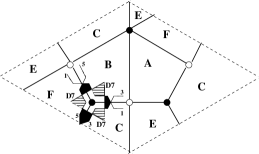
The gauge theory of D3-branes at toric singularities can be encoded in a dimer diagram [40, 41, 42, 43, 44]. This corresponds to a bi-partite tiling of $T^{2}$, where faces correspond to gauge groups, edges correspond to bi-fundamentals, and nodes correspond to superpotential terms. As an example, the dimer diagram of D3–branes on the cone over $dP_{2}$ is shown in Figure 17. As shown in [43], D3–branes on a toric singularity are mirror to D6–branes on intersecting 3-cycles in a geometry given by a fibration of a Riemann surface $\Sigma$ with punctures. This Riemann surface is just a thickening of the web diagram of the toric singularity [45, 46, 47], with punctures associated to external legs of the web diagram. The mirror D6-branes wrap non-trivial 1-cycles on this Riemann surface, with their intersections giving rise to bi-fundamental chiral multiplets, and superpotential terms arising from closed discs bounded by the D6-branes. In [19], it was shown that D7–branes passing through the singular point can be described in the mirror Riemann surface $\Sigma$ by non-compact 1-cycles which come from infinity at one puncture and go to infinity at another. Figure 18 shows the 1-cycles corresponding to some D3- and D7-branes in the Riemann surface in the geometry mirror to the complex cone over $dP_{2}$. A D7-brane leads to flavors for the two D3-brane gauge factors whose 1-cycles are intersected by the D7-brane 1-cycle, and there is a cubic coupling among the three fields (related to the disk bounded by the three 1-cycles in the Riemann surface).

Figure 17: Dimer diagram for D3–branes at a $dP_{2}$ singularity.

Figure 18: Riemann surface in the geometry mirror to the complex cone over $dP_{2}$, shown as a tiling of a $T^{2}$ with punctures (denoted by capital letters). The figure shows the non-compact 1-cycles extending between punctures, corresponding to D7-branes, and a piece of the 1-cycles that correspond to the mirror of the D3-branes.

\psfrag{Q1i}{$Q_{1i}$}\psfrag{Qi3}{$Q_{i3}$}\psfrag{Q3j}{$Q_{3j}$}\psfrag{Qj5}{$Q_{j5}$}\psfrag{Q5k}{$Q_{5k}$}\psfrag{Qk1}{$Q_{k1}$}\includegraphics[scale={2}]{dp2_flav2.eps}

Figure 19: Quiver for the $dP_{2}$ theory with M fractional branes and flavors.

As stated in Section 4, given a gauge theory of D3-branes at a toric singularity, we introduce flavors for some of the gauge factors in a specific way. We pick a term in the superpotential, and we introduce flavors for all the involved gauge factors, and coupling to all the involved bifundamental multiplets. For example, the quiver with flavors for the $dP_{2}$ theory is shown in Figure 19.

On the Riemann surface, this procedure amounts to picking a node and introducing D7-branes crossing all the edges ending on the node, see Figure 18. In this example we obtain the superpotential terms

$$W_{flavor}=\lambda^{\prime}(Q_{1i}\tilde{Q}_{i3}Y_{31}+Q_{3j}\tilde{Q}_{j5}X_{53}+Q_{5k}\tilde{Q}_{k1}X_{15})$$ (B.1)

In addition we introduce mass terms

$$W_{mass}=m_{1}Q_{1i}\tilde{Q}_{k1}+m_{2}Q_{3j}\tilde{Q}_{i3}+m_{5}Q_{5k}\tilde{Q}_{j5}$$ (B.2)

This procedure is completely general and applies to all gauge theories for branes at toric singularities.

Appendix C Detailed proof of Section 4

Recall that in Section 4 we considered the illustrative example of the gauge theory given by the quiver in Figure 20. Since node 2 is the one we wish to dualize, the only relevant part of the diagram is shown in Figure 21. We show the Seiberg dual in Figure 22.

\psfrag{X21}{$X_{21}$}\psfrag{Y21}{$Y_{21}$}\psfrag{X32}{$X_{32}$}\psfrag{Y32}{$Y_{32}$}\psfrag{Z32}{$Z_{32}$}\psfrag{X14}{$X_{14}$}\psfrag{X43}{$X_{43}$}\psfrag{Y43}{$Y_{43}$}\psfrag{Q1a}{$Q_{1a}$}\psfrag{Qa2}{$Q_{a2}$}\psfrag{Q2b}{$Q_{2b}$}\psfrag{Qb3}{$Q_{b3}$}\psfrag{Q3c}{$Q_{3c}$}\psfrag{Qc4}{$Q_{c4}$}\psfrag{Q4d}{$Q_{4d}$}\psfrag{Qd1}{$Q_{d1}$}\includegraphics[scale={0.9}]{arbquiv1.eps}

Figure 20: Quiver diagram with flavors. White nodes denote flavor groups

\psfrag{X21}{$X_{21}$}\psfrag{Y21}{$Y_{21}$}\psfrag{X32}{$X_{32}$}\psfrag{Y32}{$Y_{32}$}\psfrag{Z32}{$Z_{32}$}\psfrag{Qa2}{$Q_{a2}$}\psfrag{Q2b}{$Q_{2b}$}\includegraphics[scale={0.9}]{dualarbquiv1.eps}

Figure 21: Relevant part of quiver before Seiberg duality.

\psfrag{X12}{$\tilde{X}_{12}$}\psfrag{Y12}{$\tilde{Y}_{12}$}\psfrag{X23}{$\tilde{X}_{23}$}\psfrag{Y23}{$\tilde{Y}_{23}$}\psfrag{Z23}{$\tilde{Z}_{23}$}\psfrag{Qb2}{$\tilde{Q}_{b2}$}\psfrag{Q2a}{$\tilde{Q}_{2a}$}\psfrag{Xab}{$X_{ab}$}\psfrag{R1}{$R^{1}$}\psfrag{R2}{$R^{2}$}\psfrag{S1}{$S^{1}$}\psfrag{S2}{$S^{2}$}\psfrag{S3}{$S^{3}$}\psfrag{M1}{$M^{1},\ldots,M^{6}$}\includegraphics[scale={0.9}]{dualarbquiv2.eps}

Figure 22: Relevant part of the quiver after Seiberg duality on node 2.

The above choice of D7–branes, which we showed in appendix B can be applied to arbitrary toric singularities, gives us the superpotential terms

$$W_{flavor} = \lambda^{\prime}\,(\,X_{32}Q_{2b}Q_{b3}\,+\,X_{21}Q_{1a}Q_{a2}\,+\,X_{14}Q_{4d}Q_{d1}\,+\,Y_{43}Q_{3c}Q_{c4}\,)$$

$$W_{mass} = m_{2}Q_{a2}Q_{2b}\,+\,m_{3}Q_{b3}Q_{3c}\,+\,m_{4}Q_{c4}Q_{4d}\,+\,m_{1}Q_{d1}Q_{1a}$$ (C.1)

Taking the Seiberg dual of node 2 gives

$$W_{flavor\,dual} = \lambda^{\prime}\,(\,S^{1}_{3b}Q_{b3}\,+\,R^{1}_{a1}Q_{1a}\,+\,X_{14}Q_{4d}Q_{d1}\,+\,Y_{43}Q_{3c}Q_{c4}\,)$$

$$W_{mass\,dual} = m_{2}\underline{X_{ab}}\,+\,m_{3}Q_{b3}Q_{3c}\,+\,m_{4}Q_{c4}Q_{4d}\,+\,m_{1}Q_{d1}Q_{1a}$$

$$W_{mesons} = h\,(\,\underline{X_{ab}\tilde{Q}_{b2}\tilde{Q}_{2a}}$$

$$+ \,R^{1}_{a1}\tilde{X}_{12}\tilde{Q}_{2a}\,+\,R^{2}_{a1}\tilde{Y}_{12}\tilde{Q}_{2a}$$

$$+ \,S^{1}_{3b}\tilde{Q}_{b2}\tilde{X}_{23}\,+\,S^{2}_{3b}\tilde{Q}_{b2}\tilde{Y}_{23}\,+\,S^{3}_{3b}\tilde{Q}_{b2}\tilde{Z}_{23}$$

$$+ \,M^{1}_{31}\tilde{X}_{12}\tilde{X}_{23}\,+\,M^{2}_{31}\tilde{X}_{12}\tilde{Y}_{23}\,+\,M^{3}_{31}\tilde{X}_{12}\tilde{Z}_{23}$$

$$+ \,M^{4}_{31}\tilde{Y}_{12}\tilde{X}_{23}\,+\,M^{5}_{31}\tilde{Y}_{12}\tilde{Y}_{23}\,+\,M^{6}_{31}\tilde{Y}_{12}\tilde{Z}_{23}\,)$$ (C.2)

where we have not included the original superpotential. The crucial point is that the underlined terms appear for any quiver gauge theory with flavors introduced as described in appendix B. As described in the main text, supersymmetry is broken by the rank condition due to the F-term of the dual meson associated to the massive flavors. Our vacuum ansatz is (we take $N_{f}=2$ and $N_{c}=1$ for simplicity; this does not affect our conclusions)

$$\begin{array}[]{cc}\tilde{Q}_{b2}\,=\,\pmatrix{\mu\mathbf{1}_{N_{c}}\cr 0}&\,;\ \tilde{Q}_{2a}\,=\,(\mu\mathbf{1}_{N_{c}}\,;\,0)\end{array}$$ (C.3)

with all other vevs set to zero. We parametrize the perturbations around this minimum as

$$\begin{array}[]{ccc}\tilde{Q}_{b2}\,=\,\pmatrix{\mu+\phi_{1}\cr\phi_{2}}&\,;\ {\tilde{Q}}_{2a}\,=\,(\mu+\phi_{3}\,;\,\phi_{4})&;\ X_{ab}=\,\pmatrix{X_{00}&X_{01}\cr X_{10}&X_{11}}\end{array}$$ (C.4)

and the underlined terms give

$$hX_{ab}\tilde{Q}_{b2}\tilde{Q}_{2a}-h\mu^{2}X_{ab} = hX_{11}\,\phi_{2}\,\phi_{4}-h\mu^{2}X_{11}+h\mu\,\phi_{2}\,X_{01}+h\mu\,\phi_{4}\,X_{10}$$ (C.5)

$$+ h\mu\,\phi_{1}\,X_{00}+h\mu\,\phi_{3}\,X_{00}+h\,\phi_{1}\,\phi_{3}X_{00}+h\,\phi_{2}\,\phi_{3}X_{01}$$

$$+ h\,\phi_{1}\,\phi_{4}X_{10}$$

It is important to note that all the fields in (C.4) will have quadratic couplings only in the underlined term (C.5). Thus, one can safely study this term, and the conclusions are independent of the other terms in the superpotential. Diagonalizing (C.5) gives

$$hX_{ab}\tilde{Q}_{b2}\tilde{Q}_{2a}-h\mu^{2}X_{ab} = hX_{11}\,\phi_{2}\,\phi_{4}-h\mu^{2}X_{11}+h\mu\,\phi_{2}\,X_{01}+h\mu\,\phi_{4}\,X_{10}$$ (C.6)

$$+ \sqrt{2}h\mu\,\phi_{+}\,X_{00}+\frac{h}{2}\,\phi_{+}^{2}\,X_{00}-\frac{h}{2}\,\phi_{-}^{2}\,X_{00}$$

$$+ \frac{h}{\sqrt{2}}\,(\xi_{+}-\xi_{-})\,\phi_{2}X_{01}+\frac{h}{\sqrt{2}}\,(\xi_{+}+\xi_{-})\,\phi_{4}X_{10}$$

where

$$\xi_{+}=\frac{1}{\sqrt{2}}\,(\phi_{1}+\phi_{3})\ \ \ \ ;\ \ \ \ \xi_{-}=\frac{1}{\sqrt{2}}\,(\phi_{1}-\phi_{3})$$ (C.7)

This term is similar to the generalized asymmetric case studied in appendix A.2 with

$$X_{11}\rightarrow X\,;\,\phi_{4}\rightarrow\phi_{1}\,;\,\phi_{2}\rightarrow\phi_{2}\,;\,X_{10}\rightarrow\phi_{3}\,;\,X_{01}\rightarrow\phi_{4}\,$$ (C.8)

So here $X_{11}$ is the linear term that breaks supersymmetry, and $\phi_{2}$, $\phi_{4}$ are the broken supersymmetry fields. In (C.6), the only massless fields at tree-level are $X_{11}$ and $\xi_{-}$. Comparing to the ISS case in Section 2.1 shows that ${\rm Im}\,\xi_{-}$ is a Goldstone boson and $X_{11}$, ${\rm Re}\,\xi_{-}$ get mass at tree-level. As for $\phi_{2}$ and $\phi_{4}$, setting $\rho_{+}=\frac{1}{\sqrt{2}}(\phi_{2}+\phi_{4})$ and $\rho_{-}=\frac{1}{\sqrt{2}}(\phi_{2}-\phi_{4})$ gives us Re$(\rho_{+})$ and ${\rm Im}\,(\rho_{-})$ massless and the rest massive. Following the discussion in Section 2.1, Re$(\rho_{+})$ and ${\rm Im}\,(\rho_{-})$ are just the Goldstone bosons of the broken $SU(N_{f})$ symmetry. We have thus shown that the dualized flavors (e.g. $\tilde{Q}_{b2}$, $\tilde{Q}_{2a}$) and the meson with two flavor indices (e.g. $X_{ab}$) get mass at tree-level or at 1-loop unless they are Goldstone bosons. Now, we need to verify that this is the case for the remaining fields.

\psfrag{X14}{$X_{14}$}\psfrag{X43}{$X_{43}$}\psfrag{Y43}{$Y_{43}$}\psfrag{Q1a}{$Q_{1a}$}\psfrag{Qb3}{$Q_{b3}$}\psfrag{Q3c}{$Q_{3c}$}\psfrag{Qc4}{$Q_{c4}$}\psfrag{Q4d}{$Q_{4d}$}\psfrag{Qd1}{$Q_{d1}$}\psfrag{X12}{$\tilde{X}_{12}$}\psfrag{Y12}{$\tilde{Y}_{12}$}\psfrag{X23}{$\tilde{X}_{23}$}\psfrag{Y23}{$\tilde{Y}_{23}$}\psfrag{Z23}{$\tilde{Z}_{23}$}\psfrag{Qb2}{$\tilde{Q}_{b2}$}\psfrag{Q2a}{$\tilde{Q}_{2a}$}\psfrag{Xab}{$X_{ab}$}\psfrag{R1}{$R^{1}$}\psfrag{R2}{$R^{2}$}\psfrag{S1}{$S^{1}$}\psfrag{S2}{$S^{2}$}\psfrag{S3}{$S^{3}$}\psfrag{M1}{$M^{1}..M^{6}$}\includegraphics[scale={0.8}]{dualarbquiv3.eps}

Figure 23: Quiver after Seiberg duality on node 2.

The Seiberg dual of the original quiver diagram is shown in Figure 23. The dualized bi-fundamentals come in two classes. The first are the ones that initially (before dualizing) had cubic flavor couplings, there will always be only two of those (e.g. $\tilde{X}_{12}$, $\tilde{X}_{23}$). The second are those that did not initially have cubic couplings to flavors, there is an arbitrary number of those (e.g. $\tilde{Y}_{12}$, $\tilde{Y}_{23}$, $\tilde{Z}_{23}$). Figure 24 shows the relevant part of the quiver for the first class.

\psfrag{X12}{$\tilde{X}_{12}$}\psfrag{Y12}{$\tilde{Y}_{12}$}\psfrag{X23}{$\tilde{X}_{23}$}\psfrag{Y23}{$\tilde{Y}_{23}$}\psfrag{Z23}{$\tilde{Z}_{23}$}\psfrag{Qb2}{$\tilde{Q}_{b2}$}\psfrag{Q2a}{$\tilde{Q}_{2a}$}\psfrag{Xab}{$X_{ab}$}\psfrag{R1}{$R^{1}$}\psfrag{R2}{$R^{2}$}\psfrag{S1}{$S^{1}$}\psfrag{S2}{$S^{2}$}\psfrag{S3}{$S^{3}$}\psfrag{M1}{$M^{1},\ldots,M^{6}$}\psfrag{Q1a}{$Q_{1a}$}\psfrag{Qb3}{$Q_{b3}$}\psfrag{Q3c}{$Q_{3c}$}\psfrag{Qd1}{$Q_{d1}$}\includegraphics[scale={0.8}]{dualarbquiv4.eps}

Figure 24: Relevant part of dual quiver for first class of bi-fundamentals.

Recalling the superpotential terms (C.2), there are several possible sources of tree-level masses. For instance, these can arise in $W_{flavor\,dual}$ and $W_{mass\,dual}$. Also, remembering our assignation of vevs in (C.3), tree-level masses can also arise in $W_{mesons}$ from cubic couplings involving the broken supersymmetry fields (e.g. $\tilde{Q}_{b2}$, $\tilde{Q}_{2a}$). The first class of bi-fundamentals (e.g. $\tilde{X}_{12}$, $\tilde{X}_{23}$) only appear in $W_{mesons}$ coupled to their respective mesons (e.g. $R^{1}$, $S^{1}$). In turn these mesons will appear in quadratic terms in $W_{flavor\,dual}$ coupled to flavors (e.g. $S^{1}_{3b}Q_{b3}$ and $R^{1}_{a1}Q_{1a}$), and these flavors each appear in one term in $W_{mass}$. Thus there are two sets of three terms which are coupled at tree-level and which always couple in the same way. Consider for instance the term

$$\lambda^{\prime}\,S^{1}_{3b}Q_{b3}\,+\,m_{3}Q_{b3}Q_{3c}\,+\,h\,S^{1}_{3b}\tilde{Q}_{b2}\tilde{X}_{23} = \lambda^{\prime}\,(S_{1}\,\,S_{2})\pmatrix{B_{1}\cr B_{2}}+m_{1}(C_{1}\,\,C_{2})\pmatrix{B_{1}\cr B_{2}}$$

$$+ \,h\,(S_{1}\,\,S_{2})\pmatrix{\mu+\phi_{1}\cr\phi_{2}}\tilde{X}_{23}$$

$$= \lambda^{\prime}(S_{1}B_{1}+S_{2}B_{2})+m_{1}(B_{1}C_{1}+B_{2}C_{2})$$

$$+ h\mu\,S_{1}\,\tilde{X}_{23}\,+\,h\,S_{1}\,\phi_{1}\,\tilde{X}_{23}\,+\,h\,S_{2}\,\phi_{2}\,\tilde{X}_{23}$$

where $S_{i}$, $B_{i}$, $C_{i}$ and $\tilde{X}_{23}$ are the perturbations around the minimum. Diagonalizing (which can be done analytically for any values of the couplings), we get that all terms except one get tree-level masses, the massless field being:

$$Y=m_{1}S_{2}-\lambda^{\prime}C_{2}$$ (C.10)

This massless field has a cubic coupling to $\phi_{2}\,\tilde{X}_{23}$ and gets mass at 1-loop since $\phi_{2}$ is a broken supersymmetry field, as described in appendix A.2.

Figure 25 shows the relevant part of the quiver for the second class of bi-fundamentals (i.e. those that are dualized but do not have cubic flavor couplings).

\psfrag{X12}{$\tilde{X}_{12}$}\psfrag{Y12}{$\tilde{Y}_{12}$}\psfrag{X23}{$\tilde{X}_{23}$}\psfrag{Y23}{$\tilde{Y}_{23}$}\psfrag{Z23}{$\tilde{Z}_{23}$}\psfrag{Qb2}{$\tilde{Q}_{b2}$}\psfrag{Q2a}{$\tilde{Q}_{2a}$}\psfrag{Xab}{$X_{ab}$}\psfrag{R1}{$R^{1}$}\psfrag{R2}{$R^{2}$}\psfrag{S1}{$S^{1}$}\psfrag{S2}{$S^{2}$}\psfrag{S3}{$S^{3}$}\psfrag{M1}{$M^{1},\ldots,M^{6}$}\psfrag{Qc4}{$Q_{c4}$}\psfrag{Q4d}{$Q_{4d}$}\includegraphics[scale={0.8}]{dualarbquiv5.eps}

Figure 25: Relevant part of dual quiver for second class of bi-fundamentals.

These fields and their mesons only appear in one term, so will always couple in the same way. Taking as an example

$$h\,R^{2}_{a1}\tilde{Y}_{12}\tilde{Q}_{2a} = \pmatrix{R_{1}\cr R_{2}}\tilde{Y}_{12}\,(\mu+\phi_{3}\,;\,\phi_{4})$$ (C.11)

$$= \mu R_{1}\,\tilde{Y}_{12}\,+\,R_{1}\,\phi_{3}\,\tilde{Y}_{12}+R_{2}\,\phi_{4}\,\tilde{Y}_{12}$$

This shows that $R_{1}$ and $\tilde{Y}_{12}$ get tree-level masses and $R_{2}$ gets a mass at 1-loop since it couples to the broken supersymmetry field $\phi_{4}$. The only remaining fields are flavors like $Q_{c4}$, $Q_{4d}$, which do not transform in a gauge group adjacent to the dualized node (i.e. not adjacent in the quiver loop corresponding to the superpotential term used to introduce flavors). These are directly massive from the tree-level $W_{mass}$ term.

So, as stated, all fields except those that appear in the original superpotential (i.e. mesons with gauge indices and bi-fundamentals which are not dualized) get masses either at tree-level or at one-loop. So we only need to check the dualized original superpotential to see if we have a metastable vacua.

References

- [1] J. M. Maldacena, Adv. Theor. Math. Phys. 2, 231 (1998) [Int. J. Theor. Phys. 38, 1113 (1999)] [arXiv:hep-th/9711200].
- [2] S. S. Gubser, I. R. Klebanov and A. M. Polyakov, Phys. Lett. B 428, 105 (1998) [arXiv:hep-th/9802109].
- [3] E. Witten, Adv. Theor. Math. Phys. 2, 253 (1998) [arXiv:hep-th/9802150].
- [4] S. Kachru and E. Silverstein, Phys. Rev. Lett. 80, 4855 (1998) [arXiv:hep-th/9802183].
- [5] I. R. Klebanov and E. Witten, Nucl. Phys. B 536, 199 (1998) [arXiv:hep-th/9807080].
- [6] D. R. Morrison and M. R. Plesser, Adv. Theor. Math. Phys. 3, 1 (1999) [arXiv:hep-th/9810201].
- [7] M. Bertolini, F. Bigazzi and A. L. Cotrone, JHEP 0412, 024 (2004) [arXiv:hep-th/0411249].
- [8] S. Benvenuti, S. Franco, A. Hanany, D. Martelli and J. Sparks, JHEP 0506, 064 (2005) [arXiv:hep-th/0411264].
- [9] I. R. Klebanov and M. J. Strassler, JHEP 0008, 052 (2000) [arXiv:hep-th/0007191].
- [10] S. Franco, A. Hanany, Y. H. He and P. Kazakopoulos, arXiv:hep-th/0306092.
- [11] S. Franco, Y. H. He, C. Herzog and J. Walcher, Phys. Rev. D 70, 046006 (2004) [arXiv:hep-th/0402120].
- [12] S. Franco, A. Hanany and A. M. Uranga, JHEP 0509, 028 (2005) [arXiv:hep-th/0502113].
- [13] C. P. Herzog, Q. J. Ejaz and I. R. Klebanov, JHEP 0502, 009 (2005) [arXiv:hep-th/0412193].
- [14] D. Berenstein, C. P. Herzog, P. Ouyang and S. Pinansky, JHEP 0509, 084 (2005) [arXiv:hep-th/0505029].
- [15] S. Franco, A. Hanany, F. Saad and A. M. Uranga, JHEP 0601 (2006) 011 [arXiv:hep-th/0505040].
- [16] M. Bertolini, F. Bigazzi and A. L. Cotrone, Phys. Rev. D 72, 061902 (2005) [arXiv:hep-th/0505055].
- [17] K. Intriligator and N. Seiberg, JHEP 0602, 031 (2006) [arXiv:hep-th/0512347].
- [18] A. Brini and D. Forcella, arXiv:hep-th/0603245.
- [19] S. Franco and A. M. Uranga, JHEP 0606 (2006) 031 [arXiv:hep-th/0604136].
- [20] K. Intriligator, N. Seiberg and D. Shih, JHEP 0604 (2006) 021 [arXiv:hep-th/0602239].
- [21] B. Florea, S. Kachru, J. McGreevy and N. Saulina, arXiv:hep-th/0610003.
- [22] H. Ooguri and Y. Ookouchi, Phys. Lett. B 641 (2006) 323 [arXiv:hep-th/0607183].
- [23] R. Argurio, M. Bertolini, S. Franco and S. Kachru, JHEP 0701 (2007) 083 [arXiv:hep-th/0610212].
- [24] S. Franco, I. Garcia-Etxebarria and A. M. Uranga, JHEP 0701 (2007) 085 [arXiv:hep-th/0607218].
- [25] I. Bena, E. Gorbatov, S. Hellerman, N. Seiberg and D. Shih, JHEP 0611 (2006) 088 [arXiv:hep-th/0608157].
- [26] R. Argurio, M. Bertolini, S. Franco and S. Kachru, arXiv:hep-th/0703236.
- [27] J. D. Lykken, E. Poppitz and S. P. Trivedi, Nucl. Phys. B 543, 105 (1999) [arXiv:hep-th/9806080].
- [28] M. Wijnholt, arXiv:hep-th/0703047.
- [29] Y. E. Antebi and T. Volansky, arXiv:hep-th/0703112.
- [30] I. Garcia-Etxebarria, F. Saad and A. M. Uranga, JHEP 0608, 069 (2006) [arXiv:hep-th/0605166].
- [31] I. Garcia-Etxebarria, F. Saad and A. M. Uranga, JHEP 0606, 055 (2006) [arXiv:hep-th/0603108].
- [32] D. E. Diaconescu, B. Florea, S. Kachru and P. Svrcek, JHEP 0602, 020 (2006) [arXiv:hep-th/0512170].
- [33] K. Intriligator and N. Seiberg, arXiv:hep-ph/0702069.
- [34] S. R. Coleman and E. Weinberg, Phys. Rev. D 7 (1973) 1888.
- [35] S. Weinberg, Cambridge, UK: Univ. Pr. (1996) 489 p
- [36] J. P. Gauntlett, D. Martelli, J. Sparks and D. Waldram, Class. Quant. Grav. 21, 4335 (2004) [arXiv:hep-th/0402153].
- [37] J. P. Gauntlett, D. Martelli, J. Sparks and D. Waldram, Adv. Theor. Math. Phys. 8, 711 (2004) [arXiv:hep-th/0403002].
- [38] J. P. Gauntlett, D. Martelli, J. F. Sparks and D. Waldram, Adv. Theor. Math. Phys. 8, 987 (2006) [arXiv:hep-th/0403038].
- [39] D. Martelli and J. Sparks, Commun. Math. Phys. 262, 51 (2006) [arXiv:hep-th/0411238].
- [40] A. Hanany and K. D. Kennaway, arXiv:hep-th/0503149.
- [41] S. Franco, A. Hanany, K. D. Kennaway, D. Vegh and B. Wecht, arXiv:hep-th/0504110.
- [42] A. Hanany and D. Vegh, arXiv:hep-th/0511063.
- [43] B. Feng, Y. H. He, K. D. Kennaway and C. Vafa, arXiv:hep-th/0511287.
- [44] S. Franco and D. Vegh, arXiv:hep-th/0601063.
- [45] O. Aharony and A. Hanany, Nucl. Phys. B 504, 239 (1997) [arXiv:hep-th/9704170].
- [46] O. Aharony, A. Hanany and B. Kol, JHEP 9801, 002 (1998) [arXiv:hep-th/9710116].
- [47] N. C. Leung and C. Vafa, Adv. Theor. Math. Phys. 2, 91 (1998) [arXiv:hep-th/9711013].