Alternative Approaches to the Equilibrium Properties of Hard-Sphere Liquids

An overview of some analytical approaches to the computation of the structural and thermodynamic properties of single component and multicomponent hard-sphere fluids is provided. For the structural properties, they yield a thermodynamically consistent formulation, thus improving and extending the known analytical results of the Percus–Yevick theory. Approximate expressions for the contact values of the radial distribution functions and the corresponding analytical equations of state are also discussed. Extensions of this methodology to related systems, such as sticky hard spheres and square-well fluids, as well as its use in connection with the perturbation theory of fluids are briefly addressed.

1 Introduction

In the statistical thermodynamic approach to the theory of simple liquids, there is a close connection between the thermodynamic and structural properties BH76 ; M76 ; F85 ; HM86 . These properties depend on the intermolecular potential of the system, which is generally assumed to be well represented by pair interactions. The simplest model pair potential is that of a hard-core fluid (rods, disks, spheres, hyperspheres) in which attractive forces are completely neglected. In fact, it is a model that has been most studied and has rendered some analytical results, although up to this day no general (exact) explicit expression for the equation of state is available, except for the one-dimensional case. Something similar applies to the structural properties. An interesting feature concerning the thermodynamic properties is that in hard-core systems the equation of state depends only on the contact values of the radial distribution functions. In the absence of a completely analytical approach, the most popular methods to deal with both kinds of properties of these systems are integral equation theories and computer simulations.

It is well known that in real gases and liquids at high temperatures the state and thermodynamic properties are determined almost entirely by the repulsive forces among molecules. At lower temperatures, attractive forces become significant, but even in this case they affect very little the configuration of the system at moderate and high densities. These facts are taken into account in the application of the perturbation theory of fluids, where hard-core fluids are used as the reference systems in the computation of the thermodynamic and structural properties of real fluids. However, successful results using perturbation theory are rather limited due to the fact that, as mentioned above, there are in general no exact (analytical) expressions for the thermodynamic and structural properties of the reference systems which are in principle required in the calculations. On the other hand, in the realm of soft condensed matter the use of the hard-sphere model in connection, for instance, with sterically stabilized colloidal systems is quite common. This is due to the fact that nowadays it is possible to prepare (almost) monodisperse spherical colloidal particles with short-ranged harshly repulsive interparticle forces that may be well described theoretically with the hard-sphere potential.

This chapter presents an overview of the efforts we have made over the last few years to compute the thermodynamic and structural properties of hard-core systems using relatively simple (approximate) analytical methods. It is structured as follows. In Section 2 we describe our proposals to derive the contact values of the radial distribution functions of a multicomponent mixture (with an arbitrary size distribution, either discrete or continuous) of $d$-dimensional hard spheres from the use of some consistency conditions and the knowledge of the contact value of the radial distribution function of the corresponding single component system. In turn, these contact values lead to equations of state both for additive and non-additive hard spheres. Some consequences of such equations of state, in particular the demixing transition, are briefly analyzed. This is followed in Section 3 by the description of the Rational Function Approximation method to obtain analytical expressions for the structural quantities of three-dimensional single component and multicomponent fluids. The only required inputs in this approach are the contact values of the radial distribution functions and so the connection with the work of the previous section follows naturally. Structural properties of related systems, like sticky hard spheres or square-well fluids, that may also be tackled with the same philosophy are also discussed in Section 4. Section 5 provides an account of the reformulation of the perturbation theory of liquids using the results of the Rational Function Approximation method for a single component hard-sphere fluid and its illustration in the case of the Lennard–Jones fluid. In the final section, we provide some perspectives of the achievements obtained so far and of the challenges that remain ahead.

2 Contact Values and Equations of State for Mixtures

As stated in the Introduction, a nice feature of hard-core fluids is that the expressions of all their thermodynamic properties in terms of the radial distribution functions (RDF) are particularly simple. In fact, for these systems the internal energy reduces to that of the ideal gas and in the pressure equation it is only the contact values rather than the full RDF which appear explicitly. In this section we present our approach to the derivation of the contact values of hard-core fluid mixtures in $d$ dimensions.

2.1 Additive Systems in $d$ Dimensions

If $\sigma_{ij}$ denotes the distance of separation at contact between the centers of two interacting fluid particles, one of species $i$ and the other of species $j$, the mixture is said to be additive if $\sigma_{ij}$ is just the arithmetic mean of the hard-core diameters of each species. Otherwise, the system is non-additive. We deal in this subsection and in Subsection 2.2 with additive systems, while non-additive hard-core mixtures will be treated in Subsection 2.3.

Definitions

Let us consider an additive mixture of hard spheres (HS) in $d$ dimensions with an arbitrary number $N$ of components. In fact, our discussion will remain valid for $N\to\infty$, i.e., for polydisperse mixtures with a continuous distribution of sizes.

The additive hard core of the interaction between a sphere of species $i$ and a sphere of species $j$ is $\sigma_{ij}=\frac{1}{2}(\sigma_{i}+\sigma_{j})$, where the diameter of a sphere of species $i$ is $\sigma_{ii}=\sigma_{i}$. Let the number density of the mixture be $\rho$ and the mole fraction of species $i$ be $x_{i}=\rho_{i}/\rho$, where $\rho_{i}$ is the number density of species $i$. From these quantities one can define the packing fraction $\eta=v_{d}\rho M_{d}$, where $v_{d}=(\pi/4)^{d/2}/\Gamma(1+d/2)$ is the volume of a $d$-dimensional sphere of unit diameter and

$$M_{n}\equiv\langle\sigma^{n}\rangle=\sum_{i=1}^{N}x_{i}\sigma_{i}^{n}$$ (1)

denotes the $n$th moment of the diameter distribution.

In a HS mixture, the knowledge of the contact values $g_{ij}(\sigma_{ij})$ of the RDF $g_{ij}(r)$, where $r$ is the distance, is important for a number of reasons. For example, the availability of $g_{ij}(\sigma_{ij})$ is sufficient to get the equation of state (EOS) of the mixture via the virial expression

$$Z(\eta)=1+\frac{2^{d-1}}{M_{d}}\eta\sum_{i,j=1}^{N}x_{i}x_{j}{\sigma_{ij}^{d}}g_{ij}(\sigma_{ij}),$$ (2)

where $Z=p/\rho k_{B}T$ is the compressibility factor of the mixture, $p$ being the pressure, $k_{B}$ the Boltzmann constant, and $T$ the absolute temperature.

The exact form of $g_{ij}(\sigma_{ij})$ as functions of the packing fraction $\eta$, the set of diameters $\{\sigma_{k}\}$, and the set of mole fractions $\{x_{k}\}$ is only known in the one-dimensional case, where one simply has LZ71

$$g_{ij}(\sigma_{ij})=\frac{1}{1-\eta},\quad(d=1).$$ (3)

Consequently, for $d\geq 2$ one has to resort to approximate theories or empirical expressions. For hard-disk mixtures, an accurate expression is provided by Jenkins and Mancini’s (JM) approximation JM87 ; BS01 ,

$$g_{ij}^{\text{JM}}(\sigma_{ij})=\frac{1}{1-\eta}+\frac{9}{16}\frac{\eta}{(1-\eta)^{2}}\frac{\sigma_{i}\sigma_{j}M_{1}}{\sigma_{ij}M_{2}},\quad(d=2).$$ (4)

The associated compressibility factor is

$$Z_{\text{JM}}(\eta)=\frac{1}{1-\eta}+\frac{M_{1}^{2}}{M_{2}}\eta\frac{1+\eta/8}{(1-\eta)^{2}},\quad(d=2).$$ (5)

In the case of three-dimensional systems, some important analytical expressions for the contact values and the corresponding compressibility factor also exist. For instance, the expressions which follow from the solution of the Percus–Yevick (PY) equation of additive HS mixtures by Lebowitz L64 are

$$g_{ij}^{\text{PY}}(\sigma_{ij})=\frac{1}{1-\eta}+\frac{3}{2}\frac{\eta}{(1-\eta)^{2}}\frac{\sigma_{i}\sigma_{j}M_{2}}{\sigma_{ij}M_{3}},\quad(d=3),$$ (6)

$$Z_{\text{PY}}(\eta)=\frac{1}{1-\eta}+\frac{M_{1}M_{2}}{M_{3}}\frac{3\eta}{(1-\eta)^{2}}+\frac{M_{2}^{3}}{M_{3}^{2}}\frac{3\eta^{2}}{(1-\eta)^{2}},\quad(d=3).$$ (7)

Also analytical are the results obtained from the Scaled Particle Theory (SPT) RFL59 ; MR75 ; R88 ; HC04 ,

$$g_{ij}^{\text{SPT}}(\sigma_{ij})=\frac{1}{1-\eta}+\frac{3}{2}\frac{\eta}{(1-\eta)^{2}}\frac{\sigma_{i}\sigma_{j}M_{2}}{\sigma_{ij}M_{3}}+\frac{3}{4}\frac{\eta^{2}}{(1-\eta)^{3}}\left(\frac{\sigma_{i}\sigma_{j}M_{2}}{\sigma_{ij}M_{3}}\right)^{2},\quad(d=3),$$ (8)

$$Z_{\text{SPT}}(\eta)=\frac{1}{1-\eta}+\frac{M_{1}M_{2}}{M_{3}}\frac{3\eta}{(1-\eta)^{2}}+\frac{M_{2}^{3}}{M_{3}^{2}}\frac{3\eta^{2}}{(1-\eta)^{3}},\quad(d=3).$$ (9)

Neither the PY nor the SPT lead to particularly accurate values and so Boublík B70 and, independently, Grundke and Henderson GH72 and Lee and Levesque LL73 proposed an interpolation between the PY and the SPT contact values, that we will refer to as the BGHLL values:

$$g_{ij}^{\text{BGHLL}}(\sigma_{ij})=\frac{1}{1-\eta}+\frac{3}{2}\frac{\eta}{(1-\eta)^{2}}\frac{\sigma_{i}\sigma_{j}M_{2}}{\sigma_{ij}M_{3}}+\frac{1}{2}\frac{\eta^{2}}{(1-\eta)^{3}}\left(\frac{\sigma_{i}\sigma_{j}M_{2}}{\sigma_{ij}M_{3}}\right)^{2},\quad(d=3).$$ (10)

This leads through Eq. (2) to the widely used and rather accurate Boublík–Mansoori–Carnahan–Starling–Leland (BMCSL) EOS B70 ; MCSL71 for HS mixtures:

$$Z_{\text{BMCSL}}(\eta)=\frac{1}{1-\eta}+\frac{M_{1}M_{2}}{M_{3}}\frac{3\eta}{(1-\eta)^{2}}+\frac{M_{2}^{3}}{M_{3}^{2}}\frac{\eta^{2}(3-\eta)}{(1-\eta)^{3}},\quad(d=3).$$ (11)

Refinements of the BGHLL values have been subsequently introduced, among others, by Henderson et al. HMLC96 ; YCH96 ; HC98 ; HBCW98 ; MHC99 ; CCHW00 , Matyushov and Ladanyi ML97 , and Barrio and Solana BS00 to eliminate some drawbacks of the BMCSL EOS in the so-called colloidal limit of binary HS mixtures. On a different path, but also having to do with the colloidal limit, Viduna and Smith VS02 have proposed a method to obtain contact values of the RDF of HS mixtures from a given EOS. However, none of these proposals may be easily generalized so as to be valid for any dimensionality and any number of components. Therefore, if one wants to have a more general framework able to deal with arbitrary $d$ and $N$ an alternative strategy is called for.

Universality Ansatz

In order to follow our alternative strategy, it is useful to make use of exact limit results that can help one in the construction of approximate expressions for $g_{ij}(\sigma_{ij})$. Let us consider first the limit in which one of the species, say $i$, is made of point particles, i.e., $\sigma_{i}\rightarrow 0$. In that case, $g_{ii}(\sigma_{i})$ takes the ideal gas value, except that one has to take into account that the available volume fraction is $1-\eta$. Thus,

$$\lim_{\sigma_{i}\rightarrow 0}g_{ii}(\sigma_{i})=\frac{1}{1-\eta}.$$ (12)

An even simpler situation occurs when all the species have the same size, $\{\sigma_{k}\}\rightarrow\sigma$, so that the system becomes equivalent to a single component system. Therefore,

$$\lim_{\{\sigma_{k}\}\rightarrow\sigma}g_{ij}(\sigma_{ij})=g_{{\text{s}}},$$ (13)

where $g_{{\text{s}}}$ is the contact value of the RDF of the single component fluid at the same packing fraction $\eta$ as that of the mixture. Table 1 lists some of the most widely used proposals for the contact value $g_{\text{s}}$ and the associated compressibility factor

$$Z_{\text{s}}=1+2^{d-1}\eta g_{\text{s}}$$ (14)

in the case of the single component HS fluid.

Table 1: Some expressions of $g_{\text{s}}$ and $Z_{\text{s}}$ for the single component HS fluid. In the SHY proposal, $\eta_{\text{cp}}=(\sqrt{3}/6)\pi$ is the crystalline close-packing fraction for hard disks. In the LM proposal, $b_{3}$ and $b_{4}$ are the (reduced) third and fourth virial coefficients, $\zeta(\eta)=1.2973(59)-0.062(13)\eta/\eta_{\text{cp}}$ for $d=4$, and $\zeta(\eta)=1.074(16)+0.163(45)\eta/\eta_{\text{cp}}$ for $d=5$, where the values of the close-packing fractions are $\eta_{\text{cp}}=\pi^{2}/16\simeq 0.617$ and $\eta_{\text{cp}}=\pi^{2}\sqrt{2}/30\simeq 0.465$ for $d=4$ and $d=5$, respectively.

$d$	$g_{\text{s}}$	$Z_{\text{s}}$	Label	Ref.
$2$	$\dfrac{1-7\eta/16}{(1-\eta)^{2}}$	$\dfrac{1+\eta^{2}/8}{(1-\eta)^{2}}$	H	H75
$2$	$\dfrac{1-\eta(2\eta_{\text{cp}}-1)/2\eta_{\text{cp}}^{2}}{1-2\eta+\eta^{2}(\eta_{\text{cp}}-1)/2\eta_{\text{cp}}^{2}}$	$\dfrac{1}{1-2\eta+\eta^{2}(\eta_{\text{cp}}-1)/2\eta_{\text{cp}}^{2}}$	SHY	SHY95
$2$	$g_{{\text{s}}}^{\text{H}}-\dfrac{\eta^{3}}{2^{7}(1-\eta)^{4}}$	$Z_{{\text{s}}}^{\text{H}}-\dfrac{\eta^{4}}{2^{6}(1-\eta)^{4}}$	L	L01
$3$	$\dfrac{1+\eta/2}{(1-\eta)^{2}}$	$\dfrac{1+2\eta+3\eta^{2}}{(1-\eta)^{2}}$	PY	W63
$3$	$\dfrac{1-\eta/2+\eta^{2}/4}{(1-\eta)^{3}}$	$\dfrac{1+\eta+\eta^{2}}{(1-\eta)^{3}}$	SPT	RFL59
$3$	$\dfrac{1-\eta/2}{(1-\eta)^{3}}$	$\dfrac{1+\eta+\eta^{2}-\eta^{3}}{\left(1-\eta\right)^{3}}$	CS	CS69
$4,5$	$\dfrac{1+[2^{1-d}b_{3}-\zeta(\eta)b_{4}/b_{3}]\eta}{1-\zeta(\eta)(b_{4}/b_{3})\eta+\left[\zeta(\eta)-1\right]2^{1-d}b_{4}\eta^{2}}$	$1+2^{d-1}\eta g_{\text{s}}^{\text{LM}}$	LM	LM90

Equations (12) and (13) represent the simplest and most basic conditions that $g_{ij}(\sigma_{ij})$ must satisfy. There is a number of other less trivial consistency conditions R88 ; HMLC96 ; HC98 ; HBCW98 ; ML97 ; BS00 ; H94 ; V98 ; THM99 , some of which will be used later on.

In order to proceed, in line with a property shared by earlier proposals [see, in particular, Eqs. (4), (6), (8), and (10)], we assume that, at a given packing fraction $\eta$, the dependence of $g_{ij}(\sigma_{ij})$ on the parameters $\{\sigma_{k}\}$ and $\{x_{k}\}$ takes place only through the scaled quantity

$$z_{ij}\equiv\frac{\sigma_{i}\sigma_{j}}{\sigma_{ij}}\frac{M_{d-1}}{M_{d}}.$$ (15)

More specifically, we assume

$$g_{ij}(\sigma_{ij})=\mathcal{G}(\eta,z_{ij}),$$ (16)

where the function $\mathcal{G}(\eta,z)$ is universal in the sense that it is a common function for all the pairs $(i,j)$, regardless of the composition and number of components of the mixture. Of course, the function $\mathcal{G}(\eta,z)$ is in principle different for each dimensionality $d$. To clarify the implications of this universality ansatz, let us imagine two mixtures $\mathcal{M}$ and $\mathcal{M}^{\prime}$ having the same packing fraction $\eta$ but strongly differing in the set of mole fractions, the sizes of the particles, and even the number of components. Suppose now that there exists a pair $(i,j)$ in mixture $\mathcal{M}$ and another pair $(i^{\prime},j^{\prime})$ in mixture $\mathcal{M}^{\prime}$ such that $z_{ij}=z_{i^{\prime}j^{\prime}}$. Then, according to Eq. (16), the contact value of the RDF for the pair $(i,j)$ in mixture $\mathcal{M}$ is the same as that for the pair $(i^{\prime},j^{\prime})$ in mixture $\mathcal{M}^{\prime}$, i.e., $g_{ij}(\sigma_{ij})=g_{i^{\prime}j^{\prime}}(\sigma_{i^{\prime}j^{\prime}})$. In order to ascribe a physical meaning to the parameter $z_{ij}$, note that the ratio $M_{d-1}/M_{d}$ can be understood as a “typical” inverse diameter (or curvature) of the particles of the mixture. Thus, $z_{ij}^{-1}=\frac{1}{2}(\sigma_{i}^{-1}+\sigma_{j}^{-1})/(M_{d-1}/M_{d})$ represents the arithmetic mean curvature, in units of $M_{d-1}/M_{d}$, of a particle of species $i$ and a particle of species $j$.

Once the ansatz (16) is adopted, one may use the limits in (12) and (13) to get $\mathcal{G}(\eta,z)$ at $z=0$ and $z=1$, respectively. Since $z_{ii}\rightarrow 0$ in the limit $\sigma_{i}\rightarrow 0$, insertion of Eq. (12) into (16) yields

$$\mathcal{G}(\eta,0)=\frac{1}{1-\eta}\equiv\mathcal{G}_{0}(\eta).$$ (17)

Next, if all the diameters are equal, $z_{ij}\rightarrow 1$, so that Eq. (13) implies that

$$\mathcal{G}(\eta,1)=g_{{\text{s}}}.$$ (18)

Linear Approximation

As the simplest approximation SYH99 , one may assume a linear dependence of $\mathcal{G}$ on $z$ that satisfies the basic requirements (17) and (18), namely

$$\mathcal{G}(\eta,z)=\frac{1}{1-\eta}+\left(g_{{\text{s}}}-\frac{1}{1-\eta}\right)z.$$ (19)

Inserting this into Eq. (16), one has

$$g_{ij}^{\text{e1}}(\sigma_{ij})=\frac{1}{1-\eta}+\left(g_{{\text{s}}}-\frac{1}{1-\eta}\right)\frac{M_{d-1}}{M_{d}}\frac{\sigma_{i}\sigma_{j}}{\sigma_{ij}}.$$ (20)

Here, the label “e1” is meant to indicate that (i) the contact values used are an extension of the single component contact value $g_{{\text{s}}}$ and that (ii) $\mathcal{G}(\eta,z)$ is a linear polynomial in $z$. This notation will become handy below. Although the proposal (20) is rather crude and does not produce especially accurate results for $g_{ij}(\sigma_{ij})$ when $d\geq 3$, it nevertheless leads to an EOS that exhibits an excellent agreement with simulations in 2, 3, 4, and 5 dimensions, provided that an accurate $g_{{\text{s}}}$ is used as input SYH99 ; MV99 ; SYH01 ; GAH01 ; HYS02 . This EOS may be written as

$$Z_{\text{e1}}(\eta)=1+\frac{\eta}{1-\eta}2^{d-1}(\Omega_{0}-\Omega_{1})+\left[Z_{{\text{s}}}(\eta)-1\right]\Omega_{1},$$ (21)

where the coefficients $\Omega_{m}$ depend only on the composition of the mixture and are defined by

$$\Omega_{m}=2^{-(d-m)}\frac{M_{d-1}^{m}}{M_{d}^{m+1}}\sum_{n=0}^{d-m}\binom{d-m}{n}{M_{n+m}}{M_{d-n}}.$$ (22)

In particular, for $d=2$ and $d=3$,

$$Z_{\text{e1}}(\eta)=\frac{1}{1-\eta}+\frac{M_{1}^{2}}{M_{2}}\left[Z_{{\text{s}}}(\eta)-\frac{1}{1-\eta}\right],\quad(d=2),$$ (23)

$$Z_{\text{e1}}(\eta) = \frac{1}{1-\eta}+\frac{M_{1}M_{2}}{2M_{3}}\left\{\left[Z_{{\text{s}}}(\eta)-\frac{1}{1-\eta}\right]\left(1+\frac{M_{2}^{2}}{M_{1}M_{3}}\right)\right.$$ (24)

$$\left.+\frac{3\eta}{1-\eta}\left(1-\frac{M_{2}^{2}}{M_{1}M_{3}}\right)\right\},\quad(d=3).$$

As an extra asset, from Eq. (21) one may write the virial coefficients of the mixture $B_{n}$, defined by

$$Z=1+\sum_{n=1}^{\infty}B_{n+1}\rho^{n},$$ (25)

in terms of the (reduced) virial coefficients of the single component fluid $b_{n}$ defined by

$$Z_{\text{s}}=1+\sum_{n=1}^{\infty}b_{n+1}\eta^{n}.$$ (26)

The result is

$$B_{n}=v_{d}^{n-1}M_{d}^{n-1}\left[\Omega_{1}b_{n}+2^{d-1}(\Omega_{0}-\Omega_{1})\right].$$ (27)

In the case of binary mixtures, these coefficients are in very good agreement with the available exact and simulation results SYH99 ; SYH01 , except when the mixture involves components of very disparate sizes, especially for high dimensionalities. One may perform a slight modification such that this deficiency is avoided and thus get a modified EOS SYH01 ; S99 . For $d=2$ and $d=3$ it reads

$$Z(\eta) = Z_{\text{s}}(\eta)+x_{1}\left[\frac{1}{1-\eta_{2}}Z_{\text{s}}\left(\frac{\eta_{1}}{1-\eta_{2}}\right)-Z_{\text{s}}(\eta)\right]\left(\frac{\sigma_{2}-\sigma_{1}}{\sigma_{2}}\right)^{d-1}$$

$$+x_{2}\left[\frac{1}{1-\eta_{1}}Z_{\text{s}}\left(\frac{\eta_{2}}{1-\eta_{1}}\right)-Z_{\text{s}}(\eta)\right]\left(\frac{\sigma_{1}-\sigma_{2}}{\sigma_{1}}\right)^{d-1},\quad(d=2,3),$$

where $\eta_{i}=v_{d}\rho_{i}\sigma_{i}^{d}$ is the partial volume packing fraction due to species $i$. In contrast to most of the approaches (PY, SPT, BMCSL, e1, …), the proposal (LABEL:x50) expresses $Z(\eta)$ in terms not only of $Z_{\text{s}}(\eta)$ but also involves $Z_{\text{s}}\left(\frac{\eta_{1}}{1-\eta_{2}}\right)$ and $Z_{\text{s}}\left(\frac{\eta_{2}}{1-\eta_{1}}\right)$. Equation (LABEL:x50) should in principle be useful in particular for binary mixtures involving components of very disparate sizes. However, it is slightly less accurate than the one given in Eq. (21) for ordinary mixtures SYH01 .

Quadratic Approximation

In order to improve the proposal contained in Eq. (20), in addition to the consistency requirements (12) and (13), one may consider the condition stemming from a binary mixture in which one of the species (say $i=1$) is much larger than the other one (i.e., $\sigma_{1}/\sigma_{2}\rightarrow\infty$), but occupies a negligible volume (i.e., $x_{1}(\sigma_{1}/\sigma_{2})^{d}\rightarrow 0$). In that case, a sphere of species 1 is felt as a wall by particles of species 2, so that HMLC96 ; HBCW98 ; RDA01

$$\lim_{\stackrel{{\scriptstyle\sigma_{1}/\sigma_{2}\rightarrow\infty}}{{x_{1}(\sigma_{1}/\sigma_{2})^{d}\rightarrow 0}}}\left[g_{12}(\sigma_{12})-2^{d-1}\eta g_{22}(\sigma_{2})\right]=1.$$ (29)

Hence, in the limit considered in Eq. (29), we have $z_{22}\rightarrow 1$, $z_{12}\rightarrow 2$. Consequently, under the universality ansatz (16), one may rewrite Eq. (29) as

$$\mathcal{G}(\eta,2)=1+2^{d-1}\eta\mathcal{G}(\eta,1).$$ (30)

Thus, Eqs. (17), (18), and (30) provide complete information on the function $\mathcal{G}$ at $z=0$, $z=1$, and $z=2$, respectively, in terms of the contact value $g_{{\text{s}}}$ of the single component RDF.

The simplest functional form of $\mathcal{G}$ that complies with the above consistency conditions is a quadratic function of $z$ SYH02 :

$$\mathcal{G}(\eta,z)=\mathcal{G}_{0}(\eta)+\mathcal{G}_{1}(\eta)z+\mathcal{G}_{2}(\eta)z^{2},$$ (31)

where the coefficients $\mathcal{G}_{1}(\eta)$ and $\mathcal{G}_{2}(\eta)$ are explicitly given by

$$\mathcal{G}_{1}(\eta)=(2-2^{d-2}\eta)g_{{\text{s}}}-\frac{2-\eta/2}{1-\eta},$$ (32)

$$\mathcal{G}_{2}(\eta)=\frac{1-\eta/2}{1-\eta}-(1-2^{d-2}\eta)g_{{\text{s}}}.$$ (33)

Therefore, the explicit expression for the contact values is

$$g_{ij}^{\text{e2}}(\sigma_{ij}) = \frac{1}{1-\eta}+\left[(2-2^{d-2}\eta)g_{{\text{s}}}-\frac{2-\eta/2}{1-\eta}\right]\frac{M_{d-1}}{M_{d}}\frac{\sigma_{i}\sigma_{j}}{\sigma_{ij}}$$ (34)

$$+\left[\frac{1-\eta/2}{1-\eta}-(1-2^{d-2}\eta)g_{{\text{s}}}\right]\left(\frac{M_{d-1}}{M_{d}}\frac{\sigma_{i}\sigma_{j}}{\sigma_{ij}}\right)^{2}.$$

Following the same criterion as the one used in connection with Eq. (20), the label “e2” is meant to indicate that (i) the resulting contact values represent an extension of the single component contact value $g_{{\text{s}}}$ and that (ii) ${\mathcal{G}}(\eta,z)$ is a quadratic polynomial in $z$. Of course, the quadratic form (31) is not the only choice compatible with conditions (17), (18), and (30). For instance, a rational function was also considered in Ref. SYH02 . However, although it is rather accurate, it does not lead to a closed form for the EOS. In contrast, when Eq. (34) is inserted into Eq. (2), one gets a closed expression for the compressibility factor in terms of the packing fraction $\eta$ and the first few moments $M_{n}$, $n\leq d$. The result is

$$Z_{\text{e2}}(\eta) = 1+2^{d-2}\frac{\eta}{1-\eta}\left[2(\Omega_{0}-2\Omega_{1}+\Omega_{2})+(\Omega_{1}-\Omega_{2})\eta\right]$$ (35)

$$+\left[Z_{{\text{s}}}(\eta)-1\right]\left[2\Omega_{1}-\Omega_{2}+2^{d-2}(\Omega_{2}-\Omega_{1})\eta\right],$$

where the quantities $\Omega_{m}$ are defined in Eq. (22). Quite interestingly, in the two-dimensional case Eq. (35) reduces to Eq. (23), i.e.,

$$Z_{\text{e1}}(\eta)=Z_{\text{e2}}(\eta),\quad(d=2).$$ (36)

This illustrates the fact that two different proposals for the contact values $g_{ij}(\sigma_{ij})$ can yield the same EOS when inserted into Eq. (2). On the other hand, for three-dimensional mixtures Eq. (35) becomes

$$Z_{\text{e2}}(\eta)=\frac{1}{1-\eta}+\frac{M_{1}M_{2}}{M_{3}}\left(1-\eta+\frac{M_{2}^{2}}{M_{1}M_{3}}\eta\right)\left[Z_{{\text{s}}}(\eta)-\frac{1}{1-\eta}\right],\quad(d=3),$$ (37)

which differs from Eq. (24). In fact,

$$Z_{\text{e1}}(\eta)-Z_{\text{e2}}(\eta)=\frac{M_{1}M_{2}}{2M_{3}}\left(1-\frac{M_{2}^{2}}{M_{1}M_{3}}\right)\left[\frac{1+\eta}{1-\eta}-(1-2\eta)Z_{\text{s}}(\eta)\right],\quad(d=3).$$ (38)

Specific Examples

In this subsection, rather than carrying out an exhaustive comparison with the wealth of results available in the literature, we will consider only a few representative examples. In particular, for $d=3$, we will restrict ourselves to a comparison with classical proposals (say BGHLL, PY, and SPT for the contact values). The comparison with more recent ones may be found in Refs. SYH99 ; SYH02 ; SYH05 .

Thus far the development has been rather general since $g_{\text{s}}$ remains free in Eqs. (20) and (34). In order to get specific results, it is necessary to fix $g_{\text{s}}$ [cf. Table 1]. In the one-dimensional case, one has $g_{\text{s}}=1/(1-\eta)$ and so one gets the exact result (3) after substitution into Eq. (20). Similarly Eqs. (32) and (33) lead to $\mathcal{G}_{1}=\mathcal{G}_{2}=0$ and so we recover again the exact result.

If in the two-dimensional case we take Henderson’s value H75 $g_{\text{s}}=g_{\text{s}}^{\text{H}}$, then the linear approximation (20) reduces to the JM approximation, Eq. (4). This equivalence can be symbolically represented as $g_{ij}^{\text{eH1}}=g_{ij}^{\text{JM}}$, where the label “eH1” refers to the extension of Henderson’s single component value in the linear approximation. While $g_{ij}^{\text{JM}}$ is very accurate, even better results are provided by the quadratic form (34), especially if Luding’s value L01 $g_{\text{s}}=g_{\text{s}}^{\text{L}}$ is used LS04 .

In the three-dimensional case, Eq. (20) is of the form of the solution of the PY equation L64 . In fact, insertion of $g_{\text{s}}=g_{\text{s}}^{\text{PY}}$ leads to Eq. (6), i.e., $g_{ij}^{\text{ePY1}}=g_{ij}^{\text{PY}}$. Similarly, if the SPT expression RFL59 $g_{\text{s}}=g_{\text{s}}^{\text{SPT}}$ is used for the single component contact value in the quadratic approximation (34), we reobtain the SPT expression for the mixture, Eq. (8). In other words, $g_{ij}^{\text{eSPT2}}=g_{ij}^{\text{SPT}}$. On the other hand, if the much more accurate CS CS69 expression $g_{\text{s}}=g_{\text{s}}^{\text{CS}}$ is used as input, we arrive at the following expression:

$$g_{ij}^{\text{eCS2}}=\frac{1}{1-\eta}+\frac{3}{2}\frac{\eta(1-\eta/3)}{(1-\eta)^{2}}\frac{\sigma_{i}\sigma_{j}M_{2}}{\sigma_{ij}M_{3}}+\frac{\eta^{2}(1-\eta/2)}{(1-\eta)^{3}}\left(\frac{\sigma_{i}\sigma_{j}M_{2}}{\sigma_{ij}M_{3}}\right)^{2},\quad(d=3),$$ (39)

which is different from the BGHLL one, Eq. (10), improves the latter for $z_{ij}>1$, and leads to similar results for $z_{ij}<1$, as comparison with computer simulations shows SYH02 . The four approximations (6), (8), (10), and (39) are consistent with conditions (12) and (13), but only the SPT and eCS2 are also consistent with condition (29). It should also be noted that if one considers a binary mixture in the infinite solute dilution limit, namely $x_{1}\rightarrow 0$, so that $z_{12}\rightarrow 2/(1+\sigma_{2}/\sigma_{1})$, Eq. (39) yields the same result for $g_{12}(\sigma_{12})$ as the one proposed by Matyushov and Ladanyi ML97 for this quantity on the basis of exact geometrical relations. However, the extension that the same authors propose when there is a non-vanishing solute concentration, i.e., for $x_{1}\neq 0$, is different from Eq. (39).

Equation (34) can also be used in the case of hyperspheres ($d\geq 4$) SYH02 . In particular, a very good agreement with available computer simulations GAH01 is obtained for $d=4$ and $d=5$ by using Luban and Michels LM90 value $g_{\text{s}}=g_{\text{s}}^{\text{LM}}$.

Figure 1: Deviation of the compressibility factor from the BMCSL value, as a function of the packing fraction $\eta$ for an equimolar three-dimensional binary mixture with $\sigma_{2}/\sigma_{1}=0.6$. The open (Ref. YCH96 ) and closed (Ref. BMLS96 ) circles are simulation data. The lines are the PY EOS (– $\cdot$ $\cdot$ –), the SPT EOS (– $\cdot$ – $\cdot$), the eCS1 EOS ($\cdots$), and the eCS2 EOS (– – –).

Figure 2: Compressibility factor for three equimolar mixtures in 4D and 5D systems. Lines are the eLM1 predictions, while symbols are simulation data GAH01 .

Now we turn to the compressibility factors (21) and (35), which are obtained from the contact values (20) and (34), respectively. Since they depend on the details of the composition through the $d$ first moments, they are meaningful even for continuous polydisperse mixtures.

As said above, in the two-dimensional case both Eqs. (21) and (35) reduce to Eq. (23), which yield very accurate results when a good $Z_{\text{s}}$ is used as input HYS02 ; SYH02 ; LS04 . For three-dimensional mixtures, insertion of $Z_{\text{s}}=Z_{\text{s}}^{\text{CS}}$ in Eqs. (24) and (37) yields

$$Z_{\text{eCS1}}(\eta)=Z_{\text{BMCSL}}(\eta)+\frac{\eta^{3}M_{2}}{(1-\eta)^{3}M_{3}^{2}}\left(M_{1}M_{3}-M_{2}^{2}\right),\quad(d=3),$$ (40)

$$Z_{\text{eCS2}}(\eta)=Z_{\text{BMCSL}}(\eta)-\frac{\eta^{3}M_{2}}{(1-\eta)^{2}M_{3}^{2}}\left(M_{1}M_{3}-M_{2}^{2}\right),\quad(d=3),$$ (41)

where $Z_{\text{BMCSL}}(\eta)$ is given by Eq. (11). Note that $Z_{\text{eCS1}}(\eta)>Z_{\text{BMCSL}}(\eta)>Z_{\text{eCS2}}(\eta)$. Since simulation data indicate that the BMCSL EOS tends to underestimate the compressibility factor, it turns out that, as illustrated in Fig. 1 for an equimolar binary mixture with $\sigma_{2}/\sigma_{1}=0.6$, the performance of $Z_{\text{eCS1}}$ is, paradoxically, better than that of $Z_{\text{eCS2}}$ SYH02 , despite the fact that the underlying linear approximation for the contact values is much less accurate than the quadratic approximation. This shows that a rather crude approximation such as Eq. (20) may lead to an extremely good EOS SYH99 ; SYH01 ; GAH01 ; HYS02 , which, as clearly seen in Fig. 1, represents a substantial improvement over the classical proposals. Interestingly, the EOS corresponding to $Z_{\text{eCS1}}$ has recently been independently derived as the second order approximation of the Fundamental Measure Theory for the HS fluid by Hansen-Goos and Roth H-GR06 .

In the case of $d=4$ and $d=5$, use of $Z_{\text{s}}(\eta)=Z_{\text{s}}^{\text{LM}}(\eta)$ in Eq. (21) produces a simple extended EOS of a mixture of hard additive hyperspheres in these dimensionalities. The accuracy of these two EOS for hard hypersphere mixtures in the fluid region has been confirmed by simulation data GAH01 for a wide range of compositions and size ratios. In Fig. 2, this accuracy is explicitly exhibited in the case of three equimolar mixtures, two in $4$D and one in $5$D.

2.2 A More Consistent Approximation for Three-Dimensional Additive Mixtures

Up to this point, we have considered an arbitrary dimensionality $d$ and have constructed, under the universality assumption (16), the acurate quadratic approximation (34), which fulfills the consistency conditions (12), (13), and (29). However, there exist extra consistency conditions that are not necessarily satisfied by (34). In particular, when the mixture is in contact with a hard wall, the state of equilibrium imposes that the pressure evaluated near the wall by considering the impacts with the wall must be the same as the pressure in the bulk evaluated from the particle-particle collisions. This consistency condition is especially important if one is interested in deriving accurate expressions for the contact values of the particle-wall correlation functions.

Since a hard wall can be seen as a sphere of infinite diameter, the contact value $g_{wj}$ of the correlation function of a sphere of diameter $\sigma_{j}$ with the wall can be obtained from $g_{ij}(\sigma_{ij})$ as

$$g_{wj}=\lim_{\stackrel{{\scriptstyle\sigma_{i}\to\infty}}{{x_{i}\sigma_{i}^{d}\rightarrow 0}}}g_{ij}(\sigma_{ij}).$$ (42)

Note that $g_{wj}$ provides the ratio between the density of particles of species $j$ adjacent to the wall and the density of those particles far away from the wall. The sum rule connecting the pressure of the fluid and the above contact values is E90

$$Z_{w}(\eta)=\sum_{j=1}^{N}x_{j}g_{wj},$$ (43)

where the subscript $w$ in $Z_{w}$ has been used to emphasize that Eq. (43) represents a route alternative to the virial one, Eq. (2), to get the EOS of the HS mixture. The condition $Z=Z_{w}$ is equivalent to (29) in the special case where one has a single fluid in the presence of the wall. However, in the general case of a mixture plus a wall, the condition $Z=Z_{w}$ is stronger than Eq. (29). In the two-dimensional case, it turns out that the quadratic approximation (34) already satisfies the requirement $Z=Z_{w}$, regardless of the density and composition of the mixture LS04 . However, this is not the case for $d\geq 3$.

Our problem now consists of computing $g_{ij}(\sigma_{ij})$ and the associated $g_{wj}$ for the HS mixture in the presence of a hard wall, so that the condition $Z=Z_{w}$ is satisfied for an arbitrary mixture SYH05 . Due to the mathematical complexity of the problem, here we will restrict ourselves to three-dimensional systems ($d=3$). Similarly to what we did in the preceding subsection, we consider a class of approximations of the universal type (16), so that conditions (12) and (13) lead again to Eqs. (17) and (18), respectively. Notice that Eq. (16) implies in particular that

$$g_{wj}={\mathcal{G}}(\eta,z_{wj}),\quad z_{wj}=2\sigma_{j}\frac{M_{2}}{M_{3}}.$$ (44)

Assuming that $z=0$ is a regular point and taking into account condition (17), ${\mathcal{G}}(\eta,z)$ can be expanded in a power series in $z$:

$${\mathcal{G}}(\eta,z)={\mathcal{G}}_{0}(\eta)+\sum_{n=1}^{\infty}{\mathcal{G}}_{n}(\eta)z^{n}.$$ (45)

After simple algebra, using the ansatz (16) and Eq. (45) in Eqs. (2) (with $d=3$) and (43) one gets

$$Z={\mathcal{G}}_{0}+3\eta\frac{M_{1}M_{2}}{M_{3}}{\mathcal{G}}_{0}+4\eta\sum_{n=1}^{\infty}{\mathcal{G}}_{n}\frac{M_{2}^{n}}{M_{3}^{n+1}}\sum_{i,j=1}^{N}x_{i}x_{j}\sigma_{i}^{n}\sigma_{j}^{n}\sigma_{ij}^{3-n},$$ (46)

$$Z_{w}={\mathcal{G}}_{0}+\sum_{n=1}^{\infty}2^{n}{\mathcal{G}}_{n}\frac{M_{2}^{n}}{M_{3}^{n}}M_{n}.$$ (47)

Notice that if the series (45) is truncated after a given order $n\geq 3$, $Z_{w}$ is given by the first $n$ moments of the size distribution only. On the other hand, $Z$ still involves an infinite number of moments if the truncation is made after $n\geq 4$ due to the presence of terms like $\sum_{i,j}x_{i}x_{j}\sigma_{i}^{4}{\sigma_{j}}^{4}/\sigma_{ij}$, $\sum_{i,j}x_{i}x_{j}\sigma_{i}^{5}{\sigma_{j}}^{5}/\sigma_{ij}^{2}$, …. Therefore, if we want the consistency condition $Z=Z_{w}$ to be satisfied for any discrete or continuous polydisperse mixture, either the whole infinite series (45) needs to be considered or it must be truncated after $n=3$. The latter is of course the simplest possibility and thus we make the approximation

$${\mathcal{G}}(\eta,z)={\mathcal{G}}_{0}(\eta)+{\mathcal{G}}_{1}(\eta)z+{\mathcal{G}}_{2}(\eta)z^{2}+{\mathcal{G}}_{3}(\eta)z^{3}.$$ (48)

As a consequence, $Z$ and $Z_{w}$ depend functionally on the size distribution of the mixture only through the first three moments (which is in the spirit of Rosenfeld’s Fundamental Measure Theory R89 ).

Using the approximation (48) in Eqs. (46) and (47) we are led to

$$Z={\mathcal{G}}_{0}+\eta\left[\frac{M_{1}M_{2}}{M_{3}}\left(3{\mathcal{G}}_{0}+2{\mathcal{G}}_{1}\right)+2\frac{M_{2}^{3}}{M_{3}^{2}}\left({\mathcal{G}}_{1}+2{\mathcal{G}}_{2}+2{\mathcal{G}}_{3}\right)\right],$$ (49)

$$Z_{w}={\mathcal{G}}_{0}+2\frac{M_{1}M_{2}}{M_{3}}{\mathcal{G}}_{1}+4\frac{M_{2}^{3}}{M_{3}^{2}}\left({\mathcal{G}}_{2}+2{\mathcal{G}}_{3}\right).$$ (50)

Thus far, the dependence of both $Z$ and $Z_{w}$ on the moments $M_{1}$, $M_{2}$, and $M_{3}$ is explicit and we only lack the packing-fraction dependence of ${\mathcal{G}}_{1}$, ${\mathcal{G}}_{2}$, and ${\mathcal{G}}_{3}$. From Eqs. (49) and (50) it follows that the difference between $Z$ and $Z_{w}$ is given by

$$Z-Z_{w}=\frac{M_{1}M_{2}}{M_{3}}\left[3\eta{\mathcal{G}}_{0}-2(1-\eta){\mathcal{G}}_{1}\right]+2\frac{M_{2}^{3}}{M_{3}^{2}}\left[\eta{\mathcal{G}}_{1}-2(1-\eta){\mathcal{G}}_{2}-2(2-\eta){\mathcal{G}}_{3}\right].$$ (51)

Therefore, $Z=Z_{w}$ for any dispersity provided that

$${\mathcal{G}}_{1}(\eta)=\frac{3\eta}{2\left(1-\eta\right)^{2}},$$ (52)

$${\mathcal{G}}_{2}(\eta)=\frac{3\eta^{2}}{4\left(1-\eta\right)^{3}}-\frac{2-\eta}{1-\eta}{\mathcal{G}}_{3}(\eta),$$ (53)

where use has been made of the definition of ${\mathcal{G}}_{0}$, Eq. (17). To close the problem, we use the equal size limit given in Eq. (18), which yields $\mathcal{G}_{0}+\mathcal{G}_{1}+\mathcal{G}_{2}+\mathcal{G}_{3}=g_{\text{s}}$. After a little algebra we are led to

$${\mathcal{G}}_{2}(\eta)=(2-\eta)g_{{\text{s}}}-\frac{2+\eta^{2}/4}{\left(1-\eta\right)^{2}},$$ (54)

$${\mathcal{G}}_{3}(\eta)=(1-\eta)\left(g_{{\text{s}}}^{\text{SPT}}-g_{{\text{s}}}\right).$$ (55)

This completes the derivation of our improved approximation, which we will call “e3”, following the same criterion as the one used to call “e1” and “e2” to the approximations (20) and (34), respectively. In Eq. (55), $g_{{\text{s}}}^{\text{SPT}}$ is the SPT contact value for a single fluid, whose expression appears in Table 1. From Eq. (55) it is obvious that the choice $g_{\text{s}}=g_{{\text{s}}}^{\text{SPT}}$ makes our e3 approximation to become the e2 approximation, both reducing to the SPT for mixtures, Eq. (8). This means that the SPT is fully internally consistent with the requirement $Z=Z_{w}$, although it has the shortcoming of not being too accurate in the single component case. The e3 proposal, on the other hand, satisfies the condition $Z=Z_{w}$ and has the flexibility of accommodating any desired $g_{\text{s}}$.

For the sake of concreteness, let us write explicitly the contact values in the e3 aproximation:

$$g_{ij}^{\text{e3}}(\sigma_{ij}) = \frac{1}{1-\eta}+\frac{3\eta}{2\left(1-\eta\right)^{2}}\frac{M_{2}}{M_{3}}\frac{\sigma_{i}\sigma_{j}}{\sigma_{ij}}+\left[(2-\eta)g_{{\text{s}}}-\frac{2+\eta^{2}/4}{\left(1-\eta\right)^{2}}\right]$$ (56)

$$\times\left(\frac{M_{2}}{M_{3}}\frac{\sigma_{i}\sigma_{j}}{\sigma_{ij}}\right)^{2}+(1-\eta)\left(g_{{\text{s}}}^{\text{SPT}}-g_{{\text{s}}}\right)\left(\frac{M_{2}}{M_{3}}\frac{\sigma_{i}\sigma_{j}}{\sigma_{ij}}\right)^{3},$$

$$g_{wj}^{\text{e3}} = \frac{1}{1-\eta}+\frac{3\eta}{\left(1-\eta\right)^{2}}\frac{M_{2}}{M_{3}}\sigma_{j}+4\left[(2-\eta)g_{{\text{s}}}-\frac{2+\eta^{2}/4}{\left(1-\eta\right)^{2}}\right]\left(\frac{M_{2}}{M_{3}}\sigma_{j}\right)^{2}$$ (57)

$$+8(1-\eta)\left(g_{{\text{s}}}^{\text{SPT}}-g_{{\text{s}}}\right)\left(\frac{M_{2}}{M_{3}}\sigma_{j}\right)^{3}.$$

With the above results the compressibility factor may be finally written in terms of $Z_{{\text{s}}}$ as

$$Z_{\text{e3}}(\eta)=\frac{1}{\left(1-\eta\right)}+\left(\frac{M_{1}M_{2}}{M_{3}}-\frac{M_{2}^{3}}{M_{3}^{2}}\right)\frac{3\eta}{\left(1-\eta\right)^{2}}+\frac{M_{2}^{3}}{M_{3}^{2}}\left[Z_{\text{s}}(\eta)-\frac{1}{1-\eta}\right].$$ (58)

A few comments are in order at this stage. First, from Eq. (49) we can observe that, for the class of approximations (48), the compressibility factor $Z$ does not depend on the individual values of the coefficients $\mathcal{G}_{2}$ and $\mathcal{G}_{3}$, but only on their sum. As a consequence, two different approximations of the form (48) sharing the same density dependence of $\mathcal{G}_{1}$ and $\mathcal{G}_{2}+\mathcal{G}_{3}$ also share the same virial EOS. For instance, if one makes the choice $g_{\text{s}}=g_{\text{s}}^{\text{PY}}$, then $Z_{\text{ePY3}}=Z_{\text{PY}}$, even though $g_{ij}^{\text{ePY3}}(\sigma_{ij})\neq g_{ij}^{\text{PY}}(\sigma_{ij})$. Furthermore, if one makes the more accurate choice $g_{\text{s}}=g_{\text{s}}^{\text{CS}}$, then $Z_{\text{eCS3}}=Z_{\text{BMCSL}}$, but again $g_{ij}^{\text{eCS3}}(\sigma_{ij})\neq g_{ij}^{\text{BGHLL}}(\sigma_{ij})$. The eCS3 contact values are

$$g_{ij}^{\text{eCS3}}(\sigma_{ij}) = \frac{1}{1-\eta}+\frac{3\eta}{2\left(1-\eta\right)^{2}}\frac{M_{2}}{M_{3}}\frac{\sigma_{i}\sigma_{j}}{\sigma_{ij}}+\frac{\eta^{2}(1+\eta)}{4(1-\eta)^{3}}\left(\frac{M_{2}}{M_{3}}\frac{\sigma_{i}\sigma_{j}}{\sigma_{ij}}\right)^{2}$$ (59)

$$+\frac{\eta^{2}}{4(1-\eta)^{2}}\left(\frac{M_{2}}{M_{3}}\frac{\sigma_{i}\sigma_{j}}{\sigma_{ij}}\right)^{3},$$

$$g_{wj}^{\text{eCS3}} = \frac{1}{1-\eta}+\frac{3\eta}{\left(1-\eta\right)^{2}}\frac{M_{2}}{M_{3}}\sigma_{j}+\frac{\eta^{2}(1+\eta)}{(1-\eta)^{3}}\left(\frac{M_{2}}{M_{3}}\sigma_{j}\right)^{2}$$ (60)

$$+\frac{2\eta^{2}}{(1-\eta)^{2}}\left(\frac{M_{2}}{M_{3}}\sigma_{j}\right)^{3}.$$

Figure 3: Plot of the difference $g_{ij}(\sigma_{ij})-g_{ij}^{\text{BGHLL}}(\sigma_{ij})$ as a function of the parameter $z_{ij}=(\sigma_{i}\sigma_{j}/\sigma_{ij})M_{2}/M_{3}$ for hard spheres ($d=3$) at a packing fraction $\eta=0.49$. The symbols are simulation data for the single fluid (circle, Ref. MV99 ), three binary mixtures (squares, Ref. MBS97 ) with $\sigma_{2}/\sigma_{1}=0.3$ and $x_{1}=0.0625$, 0.125, and 0.25, and a ternary mixture (triangles, Ref. MMYSH02 ) with $\sigma_{2}/\sigma_{1}=\frac{2}{3}$, $\sigma_{3}/\sigma_{1}=\frac{1}{3}$, and $x_{1}=0.1$, $x_{2}=0.2$. The lines are the PY approximation (– $\cdot$ $\cdot$ –), the SPT approximation (– $\cdot$ – $\cdot$), the eCS1 approximation ($\cdots$), the eCS2 approximation (– – –), and the eCS3 approximation (—).

Figure 4: Plot of the difference $g_{wj}-g_{wj}^{\text{BGHLL}}$ as a function of the parameter $z_{wj}/2=\sigma_{j}M_{2}/M_{3}$ for hard spheres ($d=3$) at a packing fraction $\eta=0.4$. The symbols are simulation data for a polydisperse mixture with a narrow top-hat distribution (open squares, Ref. BPW04 ), a polydisperse mixture with a wide top-hat distribution (open circles, Ref. BPW04 ), a polydisperse mixture with a Schulz distribution (open triangles, Ref. BPW04 ), and a binary mixture (closed circles, Ref. Alexander ). The lines are the PY approximation (– $\cdot$ $\cdot$ –), the SPT approximation (– $\cdot$ – $\cdot$), the eCS1 approximation ($\cdots$), the eCS2 approximation (– – –), and the eCS3 approximation (—).

In Figs. 3 and 4 we display the performance of the contact values as given by Eqs. (59) and (60), respectively, by comparison with results of computer simulations for both discrete and polydisperse mixtures. In both figures we have also included the results that follow from the classical proposals as well as those of the eCS1 and eCS2 approximations. It is clear that for the wall-particle contact values the eCS3 approximation yields the best performance, while for the particle-particle contact values both the eCS2 and eCS3 are of comparable accuracy. A further feature to be pointed out is that the practical collapse on a common curve of the simulation data in Figs. 3 and 4 provide a posteriori support for the universality ansatz made in Eq. (16).

As mentioned earlier, there exist extra consistency conditions (see for instance Ref. HC04 ) that one might use as well within our approach. Assuming that the ansatz (16) still holds, some of these conditions are related to the derivatives of ${\mathcal{G}}$ with respect to $z$, namely

$$\left.\frac{\partial{\mathcal{G}}(\eta,z)}{\partial z}\right|_{z=0}=\frac{3\eta}{2(1-\eta)^{2}},$$ (61)

$$\left.\frac{\partial^{2}{\mathcal{G}}(\eta,z)}{\partial z^{2}}\right|_{z=0}=\frac{3\eta}{1-\eta}\left(g_{{\text{s}}}^{\text{PY}}-\frac{1}{2}g_{\text{s}}\right),$$ (62)

$$\left.\frac{\partial^{3}{\mathcal{G}}(\eta,z)}{\partial z^{3}}\right|_{z=2}=0.$$ (63)

Interestingly enough, as shown by Eq. (52), condition (61) is already satisfied by our e3 approximation without having to be imposed. On the other hand, condition (63) implies $\mathcal{G}_{3}=0$ in the e3 scheme and thus it is only satisfied if $g_{{\text{s}}}=g_{{\text{s}}}^{\text{SPT}}$, in which case we recover the SPT. Condition (62) is not fulfilled either by the SPT or by the e3 approximation (except for a particular expression of $g_{\text{s}}$ which is otherwise not very accurate). Thus, fulfilling the extra conditions (62) and (63) with a free $g_{{\text{s}}}$ requires either considering a higher order polynomial in $z$ (in which case the consistency condition $Z=Z_{w}$ cannot be satisfied for arbitrary mixtures, as discussed before) or not using the universality ansatz at all. In the first case, we have checked that a quartic or even a quintic polynomial does not improve matters, whereas giving up the universality assumption increases significantly the number of parameters to be determined and seems not to be adequate in view of the behavior observed in the simulation data.

An additional comment has to do with the restriction to $d=3$ in this subsection. As noted before, the approximation e1 reduces to the exact result (3) for $d=1$. For $d=2$, the approximation e2 already fulfills the condition $Z=Z_{w}$ and so there is no real need to go further in that case. Since we have needed the approximation e3 to satisfy $Z=Z_{w}$ for $d=3$, it is tempting to speculate that a polynomial form for $\mathcal{G}(z)$ of degree $d$ could be found to be consistent with the condition $Z=Z_{w}$ for $d\geq 4$. However, a detailed analysis shows that this is not the case for an arbitrary mixture, since the number of conditions exceeds the number of unknowns, unless the universality assumption is partially relaxed.

As a final comment, let us stress that, although the discussion in this section has referred, for the sake of simplicity, to discrete mixtures, all the dependence on the details of the composition occurs through a finite number of moments, so that the results remain meaningful even for continuous polydisperse mixtures L96 . In that case, instead of a set of mole fractions $\{x_{i}\}$ and a set of diameters $\{\sigma_{i}\}$, one has to deal with a distribution function $w(\sigma)$ such that $w(\sigma)\mathrm{d}\sigma$ is the fraction of particles with a diameter comprised between $\sigma$ and $\sigma+\mathrm{d}\sigma$. Therefore, the moments (1) are now defined as

$$M_{n}=\int_{0}^{\infty}\mathrm{d}\sigma\,\sigma^{n}w(\sigma),$$ (64)

and with such a change the results we have derived for discrete mixtures also hold for polydisperse systems.

2.3 Non-Additive Systems

Non-additive hard-core mixtures, where the distance of closest approach between particles of different species is no longer the arithmetic mean of the diameters of both particles, have received much less attention than additive mixtures, in spite of their in principle more versatility to deal with interesting aspects occurring in real systems (such as fluid-fluid phase separation) and of their potential use as reference systems in perturbation calculations on the thermodynamic and structural properties of, say, Lennard–Jones mixtures. Nevertheless, the study of non-additive systems goes back fifty years PL54 ; AO54 ; K55 and is still a rapidly developing and challenging problem.

As mentioned in the paper by Ballone et al. BPGG86 , where the relevant references may be found, experimental work on alloys, aqueous electrolyte solutions, and molten salts suggests that hetero-coordination and homo-coordination may be interpreted in terms of excluded volume effects due to non-additivity of the repulsive part of the intermolecular potential. In particular, positive non-additivity leads naturally to demixing in HS mixtures, so that some of the experimental findings of phase separation in the above mentioned (real) systems may be accounted for by using a model of a binary mixture of (positive) non-additive HS. On the other hand, negative non-additivity seems to account well for chemical short-range order in amorphous and liquid binary mixtures with preferred hetero-coordination GPE89 .

Some Preliminary Definitions

Let us consider an $N$-component mixture of non-additive HS in $d$ dimensions. In this case, $\sigma_{ij}=\frac{1}{2}(\sigma_{i}+\sigma_{j})(1+\Delta_{ij})$, where $\Delta_{ij}\geq-1$ is a symmetric matrix with zero diagonal elements ($\Delta_{ii}=0$) that characterizes the degree of non-additivity of the interactions. If $\Delta_{ij}>0$ the non-additivity character of the $ij$ interaction is said to be positive, while it is negative if $\Delta_{ij}<0$. In the case of a binary mixture ($N=2$), the only non-additivity parameter is $\Delta\equiv\Delta_{12}=\Delta_{21}$. The virial EOS (2) remains being valid in the non-additive case.

The contact values $g_{ij}(\sigma_{ij})$ can be expanded in a power series in density as

$$g_{ij}(\sigma_{ij})=1+v_{d}\rho\sum_{k=1}^{N}x_{k}c_{k;ij}+(v_{d}\rho)^{2}\sum_{k,\ell=1}^{N}x_{k}x_{\ell}c_{k\ell;ij}+\mathcal{O}(\rho^{3}).$$ (65)

The coefficients $c_{k;ij}$, $c_{k\ell;ij}$, …are independent of the composition of the mixture, but they are in general complicated nonlinear functions of the diameters $\sigma_{ij}$, $\sigma_{ik}$, $\sigma_{jk}$, $\sigma_{k\ell}$, …. Insertion of the expansion (65) into Eq. (2) yields the virial expansion of $Z$, namely

$$Z(\rho) = 1+\sum_{n=2}^{\infty}\overline{B}_{n}(v_{d}\rho)^{n-1}$$ (66)

$$= 1+v_{d}\rho\sum_{i,j=1}^{N}\overline{B}_{ij}x_{i}x_{j}+(v_{d}\rho)^{2}\sum_{i,j,k=1}^{N}\overline{B}_{ijk}x_{i}x_{j}x_{k}$$

$$+(v_{d}\rho)^{3}\sum_{i,j,k,\ell=1}^{N}\overline{B}_{ijk\ell}x_{i}x_{j}x_{k}x_{\ell}+\mathcal{O}(\rho^{4}).$$

Note that, for further convenience, we have introduced the coefficients $\overline{B}_{n}\equiv v_{d}^{-(n-1)}B_{n}$, where $B_{n}$ are the usual virial coefficients [cf. Eq. (25)]. The composition-independent second, third, and fourth (barred) virial coefficients are given by

$$\overline{B}_{ij}=2^{d-1}\sigma_{ij}^{d},$$ (67)

$$\overline{B}_{ijk}=\frac{2^{d-1}}{3}\left(c_{k;ij}\sigma_{ij}^{d}+c_{j;ik}\sigma_{ik}^{d}+c_{i;jk}\sigma_{jk}^{d}\right),$$ (68)

$$\overline{B}_{ijk\ell} = \frac{2^{d-1}}{6}\left(c_{k\ell;ij}\sigma_{ij}^{d}+c_{j\ell;ik}\sigma_{ik}^{d}+c_{i\ell;jk}\sigma_{jk}^{d}+c_{jk,i\ell}\sigma_{i\ell}^{d}+c_{ik,j\ell}\sigma_{j\ell}^{d}\right.$$ (69)

$$\left.+c_{ij;k\ell}\sigma_{k\ell}^{d}\right).$$

A Simple Proposal for the Equation of State of $d$-Dimensional Non-Additive Mixtures

Our goal now is to generalize the e1 proposal given by Eq. (20) to the non-additive case SHY05 . We will not try to extend the e2 and e3 proposals, Eqs. (34) and (56), because of two reasons. First, given the inherent complexity of non-additive systems, we want to keep the approach as simple as possible. Second, we are more interested in the EOS than in the contact values themselves and, as mentioned earlier, the e1 proposal provides excellent EOS, at least in the additive case, despite the simplicity of the corresponding contact values.

As the simplest possible extension, we impose again the point particle and equal size consistency conditions, Eqs. (12) and (13), and thus keep in this case also the ansatz (16) and the linear structure of Eq. (19). However, instead of using Eq. (15), we determine the parameters $z_{ij}$ as to reproduce Eq. (65) to first order in the density. The result is readily found to be SHY05

$$z_{ij}=\left(\frac{b_{3}}{b_{2}}-1\right)^{-1}\left(\frac{\sum_{k}x_{k}c_{k;ij}}{M_{d}}-1\right).$$ (70)

Here $b_{2}=2^{d-1}$ and $b_{3}$ are the second and third virial coefficients for the single component fluid, as defined by Eq. (26). The proposal of Eq. (19) supplemented by Eq. (70) is, by construction, accurate for densities low enough as to justify the truncated approximation $g_{ij}(\sigma_{ij})\approx 1+v_{d}\rho\sum_{k}x_{k}c_{k;ij}$. On the other hand, the limitations of this truncated expansion for moderate and large densities may be compensated by the use of $g_{{\text{s}}}$. When Eqs. (16), (19), and (70) are inserted into Eq. (2) one gets

$$Z(\eta)=1+\frac{\eta}{1-\eta}\frac{b_{3}M_{d}\overline{B}_{2}-b_{2}\overline{B}_{3}}{(b_{3}-b_{2})M_{d}^{2}}+\left[Z_{{\text{s}}}(\eta)-1\right]\frac{\overline{B}_{3}-M_{d}\overline{B}_{2}}{(b_{3}-b_{2})M_{d}^{2}}.$$ (71)

Equation (71) is the sought generalization of Eq. (21) to non-additive hard-core systems. As in the additive case, the the density dependence in the EOS of the mixture is rather simple: $Z(\eta)-1$ is expressed as a linear combination of $\eta/(1-\eta)$ and $Z_{{\text{s}}}(\eta)-1$, with coefficients such that the second and third virial coefficients are reproduced. Again, Eq. (71) is bound to be accurate for sufficiently low densities, while the limitations of the truncated expansion for moderate and large densities are compensated by the use of the EOS of the pure fluid.

The exact second virial coefficient $\overline{B}_{2}$ is known from Eq. (67). In principle, one should use the exact coefficients $c_{k;ij}$ to compute $\overline{B}_{3}$. However, to the best of our knowledge they are only known for $d\leq 3$. Since our objective is to have a proposal which is explicit for any $d$, we can make use of a reasonable approximation for them SHY05 , as described below.

An Approximate Proposal for $c_{k;ij}$

The values of the coefficients $c_{k;ij}$ are exactly known for $d=1$ and $d=3$ and from these results one may approximate them in $d$ dimensions as SHY05

$$c_{k;ij}=\sigma_{k;ij}^{d}+\left(\frac{b_{3}}{b_{2}}-1\right)\frac{\sigma_{k;ij}^{d-1}}{\sigma_{ij}}\sigma_{i;jk}\sigma_{j;ik},$$ (72)

where we have called

$$\sigma_{k;ij}\equiv\sigma_{ik}+\sigma_{jk}-\sigma_{ij}$$ (73)

and it is understood that $\sigma_{k;ij}\geq 0$ for all sets $ijk$. Clearly, $\sigma_{i;ij}=\sigma_{i}$. For a binary mixture Eq. (72) yields

$$\begin{array}[]{l}c_{1;11}=({b_{3}}/{b_{2}})\sigma_{1}^{d},\\ c_{2;11}=(2\sigma_{12}-\sigma_{1})^{d}+\left({b_{3}}/{b_{2}}-1\right)\sigma_{1}(2\sigma_{12}-\sigma_{1})^{d-1},\\ c_{1;12}={\sigma}_{1}^{d}+\left({b_{3}}/{b_{2}}-1\right){(2\sigma_{12}-\sigma_{1})\sigma_{1}^{d}}/{\sigma_{12}}.\end{array}$$ (74)

Of course, Eqs. (72) and (74) reduce to the exact results for $d=1$ ($b_{2}=b_{3}=1$) and for $d=3$ ($b_{2}=4$, $b_{3}=10$).

The quantities $\sigma_{k;ij}$ may be given a simple geometrical interpretation. Assume that we have three spheres of species $i$, $j$, and $k$ aligned in the sequence $ikj$. In such a case, the distance of closest approach between the centers of spheres $i$ and $j$ is $\sigma_{ik}+\sigma_{jk}$. If the sphere of species $k$ were not there, that distance would of course be $\sigma_{ij}$. Therefore $\sigma_{k;ij}$ as given by Eq. (73) represents a kind of effective diameter of sphere $k$, as seen from the point of view of the interaction between spheres $i$ and $j$.

Inserting Eq. (72) into Eq. (70), one gets

$$z_{ij}=\left(\frac{b_{3}}{b_{2}}-1\right)^{-1}\left(\frac{\sum_{k}x_{k}\sigma_{k;ij}^{d}}{M_{d}}-1\right)+\frac{\sum_{k}x_{k}\sigma_{k;ij}^{d-1}\sigma_{i;jk}\sigma_{j;ik}}{M_{d}\sigma_{ij}}.$$ (75)

It can be easily checked that in the additive case ($\sigma_{k;ij}\to\sigma_{k}$), Eq. (75) reduces to Eq. (15).

Equations (72) and (74) are restricted to the situation $\sigma_{k;ij}\geq 0$ for any choice of $i$, $j$, and $k$, i.e., $2\sigma_{12}\geq\text{max}(\sigma_{1},\sigma_{2})$ in the binary case. This excludes the possibility of dealing with mixtures with extremely high negative non-additivity in which one sphere of species $k$ might “fit in” between two spheres of species $i$ and $j$ in contact. Since for $d=3$ and $N=2$ the coefficients $c_{k;ij}$ are also known for such mixtures H96b , we may extend our proposal to deal with these cases:

$$\begin{array}[]{l}c_{1;11}=(b_{3}/{b_{2}})\sigma_{1}^{d},\\ c_{2;11}=\widehat{\sigma}_{2}^{d}+\left({b_{3}}/{b_{2}}-1\right)\sigma_{1}\widehat{\sigma}_{2}^{d-1},\\ c_{1;12}=(2\sigma_{12}-\widehat{\sigma}_{2})^{d}+\left({b_{3}}/{b_{2}}-1\right){\widehat{\sigma}_{2}\sigma_{1}^{d}}/{\sigma_{12}},\end{array}$$ (76)

where we have defined

$$\widehat{\sigma}_{2}=\text{max}\left(2\sigma_{12}-\sigma_{1},0\right).$$ (77)

With such an extension, we recover the exact values of $c_{k;ij}$ for a binary mixture of hard spheres ($d=3$), even if $\sigma_{1}>2\sigma_{12}$ or $\sigma_{2}>2\sigma_{12}$.

The EOS (71) becomes explicit when $\overline{B}_{3}$ is obtained from Eq. (68) by using the approximation (72). The resulting virial coefficient is the exact one for $d=1$ and $d=3$. For hard disks ($d=2$), it turns out that the approximate third virial coefficient is practically indistinguishable from the exact one SHY05 . When the approximate $\overline{B}_{3}$ is used, Eq. (71) reduces to Eq. (21) in the additive case.

Figure 5: Plot of the compressibility factor versus the non-additivity parameter $\Delta$ for a symmetric binary mixture of non-additive hard spheres ($d=3$) at $\eta=\pi/30$ and two different compositions. The solid lines are our proposal, Eq. (71), with $Z_{\text{s}}=Z_{\text{s}}^{\text{CS}}$, while the dashed lines are Hamad’s proposal (Refs. H96a ; H96c ; H99 ). The symbols are results from Monte Carlo simulations (Refs. JJR94a ; JJR94b ).

From the comparison with simulation results, both for the compressibility factor and higher order virial coefficients, we find that the EOS (71) does a good job for non-additive mixtures, thus representing a reasonable compromise between simplicity and accuracy, provided that $Z_{{\text{s}}}$ is accurate enough. This is illustrated in Fig. 5, where the proposal (71) with $Z_{\text{s}}=Z_{\text{s}}^{\text{CS}}$ and a similar proposal by Hamad H96a ; H96c ; H99 are compared with simulation data JJR94a ; JJR94b for some three-dimensional symmetric mixtures. A more extensive comparison SHY05 shows that Eq. (71) seems to work better (especially as the density is increased) in the case of positive non-additivities, at least for $d=1$, $d=2$, and $d=3$, but its performance is also reasonably good in highly asymmetric mixtures, even for negative $\Delta$. Of course the full assessment of this proposal is still pending since it involves many facets (non-additivity parameters, size ratios, density, and composition). Without this full assessment and given its rather satisfactory performance so far, going beyond the approximation given by Eq. (19) (taking similar steps to the ones described in Subsections 2.1 and 2.2 for additive systems) does not seem to be necessary at this stage, although it is in principle feasible.

2.4 Demixing

Demixing is a common phase transition in fluid mixtures usually originated on the asymmetry of the interactions (e.g., their strength and/or range) between the different components in the mixture. In the case of athermal systems such as HS mixtures in $d$ dimensions, if fluid-fluid separation occurs, it would represent a neat example of an entropy-driven phase transition, i.e., a phase separation based only on the size asymmetry of the components. The existence of demixing in binary additive three dimensional HS mixtures has been studied theoretically since decades, and the issue is still controversial. In this subsection we will present our results following different but related routes that attempt to clarify some aspects of this problem.

Binary Mixtures of Additive $d$-Dimensional Spheres ($d=3$, $d=4$ and $d=5$)

Now we look at the possible instability of a binary fluid mixture of HS of diameters $\sigma_{1}$ and $\sigma_{2}$ ($\sigma_{1}>\sigma_{2}$) in $d$ dimensions by looking at the Helmholtz free energy per unit volume, $f$, which is given by

$$\frac{f}{\rho k_{B}T}=-1+\sum_{i=1}^{2}x_{i}\ln\left(x_{i}\rho\lambda_{i}^{d}\right)+\int_{0}^{\eta}\mathrm{d}\eta^{\prime}\frac{Z(\eta^{\prime})-1}{\eta^{\prime}},$$ (78)

where $\lambda_{i}$ is the thermal de Broglie wavelength of species $i$. We locate the spinodals through the condition $f_{11}f_{22}-f_{12}^{2}=0$, with $f_{ij}\equiv\partial^{2}{f}/\partial\rho_{i}\partial\rho_{j}$. Due to the spinodal instability, the mixture separates into two phases of different composition. The coexistence conditions are determined through the equality of the pressure $p$ and the two chemical potentials $\mu_{1}$ and $\mu_{2}$ in both phases ($\mu_{i}=\partial{f}/\partial\rho_{i}$), leading to binodal (or coexistence) curves.

We begin with the case $d=3$. It is well known that the BMCSL EOS, Eq. (11), does not lead to demixing. However, other EOS for HS mixtures have been shown to predict demixing RDA01 ; CB98b , including the EOS that is obtained by truncating the virial series after a certain number of terms VM03 ; HT04 . In particular, it turns out that both $Z=Z_{\text{eCS1}}$, Eq. (40), and $Z=Z_{\text{eCS2}}$, Eq. (41), lead to demixing for certain values of the parameter $\gamma\equiv{\sigma_{2}}/{\sigma_{1}}$ that measures the size asymmetry. The critical values of the pressure, the composition, and the packing fraction are presented in Table 2 for a few values of $\gamma$.

Table 2: Critical constants ${p_{c}\sigma_{1}^{3}}/{k_{B}T}$, $x_{1c}$, and $\eta_{c}$ for different $\gamma$-values as obtained from the two extended CS equations (40) and (41).

	eCS1			eCS2
$\gamma$	$p_{c}\sigma_{1}^{3}/k_{B}T$	$x_{1c}$	$\eta_{c}$	$p_{c}\sigma_{1}^{3}/k_{B}T$	$x_{1c}$	$\eta_{c}$
0.05	3599	0.0093	0.822	1096	0.0004	0.204
0.1	1307	0.0203	0.757	832.0	0.0008	0.290
0.2	653.4	0.0537	0.725	—	—	—
0.3	581.9	0.0998	0.738	—	—	—
0.4	663.4	0.1532	0.766	—	—	—

As discussed earlier, the eCS1 EOS and, to a lesser extent, the eCS2 EOS are both in reasonably good agreement with the available simulation results for the compressibility factor YCH96 ; MV99 ; BMLS96 and lead to the exact second and third virial coefficients but differ in the predictions for $B_{n}$ with $n\geq 4$. The scatter in the values for the critical constants shown in Table 2 is evident and so there is no indication as to whether one should prefer one equation over the other in connection with this problem. Notice, for instance, that the eCS2 does not predict demixing for $\gamma\geq 0.2$, while both the values of the critical pressures and packing fractions for which it occurs according to the eCS1 EOS suggest that the transition might be metastable with respect to a fluid-solid transition.

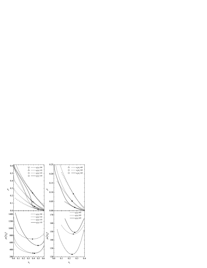
Figure 6: Spinodal curves (upper panels: lines) and binodal curves (upper panels: open symbols; lower panels: lines) in a 4D system (left panels) and in a 5D system (right panels). The closed symbols are the critical consolute points.

Now we turn to the cases $d=4$ and $d=5$. Here we use the extended Luban–Michels equation (eLM1) described in Subsection 2.1 [see Eq. (21) and Table 1]. As seen in Fig. 6, the location of the critical point tends to go down and to the right in the $\eta_{2}$ vs $\eta_{1}$ plane as $\gamma$ decreases for $d=4$ YSH00a . On the other hand, while it also tends to go down as $\gamma$ decreases if $d=5$, its behavior in the $\eta_{2}$ vs $\eta_{1}$ plane is rather more erratic in this case. Also, the value of the critical pressure $p_{\text{c}}$ (in units of $k_{B}T/\sigma_{1}^{d}$) is not a monotonic function of $\gamma$; its minimum value lies between $\gamma=1/3$ and $\gamma=1/2$ when $d=4$, and it is around $\gamma=3/5$ for $d=5$. This non-monotonic behavior is also observed for three-dimensional HS CB98b ; HT04 .

It is conceivable that the demixing transition in binary mixtures of hard hyperspheres in four and five dimensions described above may be metastable with respect to a fluid-solid transition, as it may also be the case of 3D HS. In fact, the value of the pressure at the freezing transition for the single component fluid is LM90 $p_{\text{f}}\sigma^{d}/k_{B}T\simeq 12.7$ ($d=3$), 11.5 ($d=4$), and 12.2 ($d=5$), i.e., $p_{\text{f}}\sigma^{d}/k_{B}T$ does not change appreciably with the dimensionality but is clearly very small in comparison with the critical pressures $p_{\text{c}}\sigma_{1}^{d}/k_{B}T$ we obtain for the mixture; for instance, $p_{\text{c}}\sigma_{1}^{d}/k_{B}T\simeq 600$ ($d=3$, $\gamma=3/10$), 300 ($d=4$, $\gamma=1/3$) and 123 ($d=5$, $\gamma=3/5$). However, one should also bear in mind that, if the concentration $x_{1}$ of the bigger spheres decreases, the value of the pressure at which the solid-fluid transition in the mixture occurs in 3D is also considerably increased with respect to $p_{\text{f}}$ [cf. Fig. 6 of Ref. CB98b ]. Thus, for concentrations $x_{1}\simeq 0.01$ corresponding to the critical point of the fluid-fluid transition, the maximum pressure of the fluid phase greatly exceeds $p_{\text{f}}$. If a similar trend with composition also holds in 4D and 5D, and given that the critical pressures become smaller as the dimensionality $d$ is increased, it is not clear whether the competition between the fluid-solid and the fluid-fluid transitions in these dimensionalities will always be won by the former. The point clearly deserves further investigation.

An interesting feature must be mentioned. There is a remarkable similarity between the binodal curves represented in the $p\sigma_{i}^{d}$–$\eta_{1}$ and in the $\mu_{i}$–$\eta_{1}$ planes YSH00a . By eliminating $\eta_{1}$ as if it were a parameter, one can represent the binodal curves in a $\mu_{i}$ vs $p\sigma_{i}^{d}$ plane. Provided the origin of the chemical potentials is such as to make $\lambda_{i}=\sigma_{i}$, the binodals in the $\mu_{i}$–$p\sigma_{i}^{d}$ plane practically collapse into a single curve (which is in fact almost a straight line) for each dimensionality ($d=3$, $d=4$, and $d=5$) YSH00a . A closer analysis of this phenomenon shows, however, that it is mainly due to the influence on $\mu_{i}$ of terms which are quantitatively dominant but otherwise irrelevant to the coexistence conditions.

Binary Mixtures of Non-Additive Hard Hyperspheres in the Limit of High Dimensionality

Let us now consider a binary mixture of non-additive HS of diameters $\sigma_{1}$ and $\sigma_{2}$ in $d$ dimensions. Thus in this case $\sigma_{12}\equiv\frac{1}{2}(\sigma_{1}+\sigma_{2})(1+\Delta)$ where as before $\Delta$ may be either positive or negative. Further assume (something that will become exact in the limit $d\to\infty$ CFP91 ) that the EOS of the mixture is described by the second virial coefficient only, namely

$$p=\rho k_{B}T\left[1+B_{2}(x_{1})\rho\right],$$ (79)

where, according to Eq. (67),

$$B_{2}(x_{1})=v_{d}2^{d-1}\left(x_{1}^{2}\sigma_{1}^{d}+x_{2}^{2}\sigma_{2}^{d}+2x_{1}x_{2}\sigma_{12}^{d}\right).$$ (80)

The Helmholtz free energy per unit volume is given by ${f}/{\rho k_{B}T}=-1+\sum_{i=1}^{2}x_{i}\ln\left(x_{i}\rho\lambda_{i}^{d}\right)+B_{2}\rho$, where Eq. (78) has been used. The Gibbs free energy per particle is

$$g=(f+p)/\rho=\sum_{i=1}^{2}x_{i}\ln\left(x_{i}\rho\lambda_{i}^{d}\right)+2B_{2}(x_{1})\rho,$$ (81)

where without loss of generality we have set $k_{B}T=1$. Given a size ratio $\gamma$, a value of $\Delta$, and a dimensionality $d$, the consolute critical point $(x_{1c},p_{c})$ is the solution to $\left({\partial^{2}g}/{\partial x_{1}^{2}}\right)_{p}=\left({\partial^{3}g}/{\partial x_{1}^{3}}\right)_{p}=0$, provided of course it exists. Then, one can get the critical density $\rho_{c}$ from Eq. (79).

We now introduce the scaled quantities SH05

$$\widetilde{p}\equiv 2^{d-1}v_{d}d^{-2}p\sigma_{1}^{d}/k_{B}T,\quad u\equiv d^{-1}B_{2}\rho.$$ (82)

Consequently, Eqs. (79) and (81) can be rewritten as

$$\widetilde{p}=u\left(u+d^{-1}\right)/{\widetilde{B}_{2}},$$ (83)

$$g=\sum_{i=1}^{2}x_{i}\ln\left(x_{i}\Lambda_{i}\right)+\ln\left({A_{d}u}/{\widetilde{B}_{2}}\right)+2du,$$ (84)

where $\widetilde{B}_{2}\equiv B_{2}/2^{d-1}v_{d}\sigma_{1}^{d}$, $\Lambda_{i}\equiv(\lambda_{i}/\sigma_{1})^{d}$, and $A_{d}\equiv d/2^{d-1}v_{d}$. Next we take the limit $d\to\infty$ and assume that the volume ratio $\widetilde{\gamma}\equiv\gamma^{d}$ is kept fixed and that there is a (slight) non-additivity $\Delta=d^{-2}\widetilde{\Delta}$ such that the scaled non-additivity parameter $\widetilde{\Delta}$ is also kept fixed in this limit. Thus, the second virial coefficient can be approximated by

$$\widetilde{B}_{2}=\widetilde{B}_{2}^{(0)}+\widetilde{B}_{2}^{(1)}d^{-1}+\mathcal{O}(d^{-2}),\quad\widetilde{B}_{2}^{(0)}=\left(x_{1}+x_{2}\widetilde{\gamma}^{1/2}\right)^{2},\quad\widetilde{B}_{2}^{(1)}=x_{1}x_{2}\widetilde{\gamma}^{1/2}J,$$ (85)

with

$$J\equiv\frac{1}{4}\left(\ln\widetilde{\gamma}\right)^{2}+2\widetilde{\Delta}.$$ (86)

Let us remark that, in order to find a consolute critical point, it is essential to keep the term of order $d^{-1}$ if $\widetilde{\Delta}\leq 0$. The EOS (83) can then be inverted to yield

$$u=u^{(0)}+u^{(1)}d^{-1}+\mathcal{O}(d^{-2}),\quad u^{(0)}=\sqrt{\widetilde{p}\widetilde{B}_{2}^{(0)}},\quad u^{(1)}=-\frac{1}{2}\left(1-u^{(0)}\frac{\widetilde{B}_{2}^{(1)}}{\widetilde{B}_{2}^{(0)}}\right).$$ (87)

In turn, the Gibbs free energy (84) becomes

$$\begin{array}[]{ll}&g=g^{(0)}d+g^{(1)}+\mathcal{O}(d^{-1}),\\ &g^{(0)}=2u^{(0)},\quad g^{(1)}=\sum_{i=1}^{2}x_{i}\ln\left(x_{i}\Lambda_{i}\right)+\ln\left(A_{d}{u^{(0)}}/{\widetilde{B}_{2}^{(0)}}\right)+2u^{(1)},\end{array}$$ (88)

while the chemical potentials $\mu_{1}=g+x_{2}\left(\partial g/\partial x_{1}\right)_{p}$ and $\mu_{2}=g-x_{1}\left(\partial g/\partial x_{1}\right)_{p}$ are given by

$$\begin{array}[]{ll}&\mu_{i}=\mu_{i}^{(0)}d+\mu_{i}^{(1)}+\mathcal{O}(d^{-1}),\quad\mu_{1}^{(0)}=2\widetilde{p}^{1/2},\\ &\mu_{1}^{(1)}=\ln\left(A_{d}x_{1}\Lambda_{1}\sqrt{\widetilde{p}/\widetilde{B}_{2}^{(0)}}\right)-1/\sqrt{\widetilde{B}_{2}^{(0)}}+(x_{2}/x_{1})(\widetilde{\gamma}\widetilde{p})^{1/2}\widetilde{B}_{2}^{(1)}/\widetilde{B}_{2}^{(0)},\end{array}$$ (89)

where $\mu_{2}$ is obtained from $\mu_{1}$ by the changes $x_{1}\leftrightarrow x_{2}$, $\Lambda_{1}\to\Lambda_{2}/\widetilde{\gamma}$, $\widetilde{\gamma}\to 1/\widetilde{\gamma}$, $\widetilde{p}\to\widetilde{p}\widetilde{\gamma}$, $\widetilde{B}_{2}\to\widetilde{B}_{2}/\widetilde{\gamma}$.

The coordinates of the critical point are readily found to be

$$x_{1c}=\frac{\widetilde{\gamma}^{3/4}}{1+\widetilde{\gamma}^{3/4}},\quad\widetilde{p}_{c}=\frac{\left(1+\widetilde{\gamma}^{1/4}\right)^{4}}{4\widetilde{\gamma}J^{2}}.$$ (90)

Note that $x_{1c}$ is independent of $\widetilde{\Delta}$. The coexistence curve, which has to be obtained numerically, follows from the conditions $\mu_{i}^{(1)}(x_{A},\widetilde{p})=\mu_{i}^{(1)}(x_{B},\widetilde{p})$ ($i=1,2$) where $x_{1}=x_{A}$ and $x_{1}=x_{B}$ are the mole fractions of the coexisting phases. Once the critical consolute point has been identified in the pressure/concentration plane, we can obtain the critical density. The dominant behaviors of $\widetilde{B}_{2}$ and $u$ at the critical point are

$$\widetilde{B}_{2}^{(0)}(x_{1c})=\frac{\widetilde{\gamma}}{\left(1-\widetilde{\gamma}^{1/4}+\widetilde{\gamma}^{1/2}\right)^{2}},\quad u_{c}^{(0)}=\frac{\left(1+\widetilde{\gamma}^{1/4}\right)^{2}}{2\left(1-\widetilde{\gamma}^{1/4}+\widetilde{\gamma}^{1/2}\right)J}.$$ (91)

Hence, the critical density readily follows after substitution in the scaling relation given in Eq. (82). It is also convenient to consider the scaled version $\widetilde{\eta}\equiv d^{-1}2^{d}\eta$ of the packing fraction $\eta=v_{d}\rho\sigma_{1}^{d}\left(x_{1}+x_{2}\widetilde{\gamma}\right)$. At the critical point, it takes the nice expression

$$\widetilde{\eta}_{c}=\frac{\left(\widetilde{\gamma}^{1/8}+\widetilde{\gamma}^{-1/8}\right)^{2}}{J}.$$ (92)

Figure 7: Binodal curves in the planes $\widetilde{p}$ vs $x_{1}$ and $\widetilde{\eta}$ vs $x_{1}$ corresponding to $\widetilde{\gamma}=0.01$ and $\widetilde{\Delta}=-0.1$, $\widetilde{\Delta}=0$, and $\widetilde{\Delta}=0.1$.

The previous results clearly indicate that a demixing transition is possible not only for additive or positively non-additive mixtures but even for negative non-additivities. The only requirement is $J>0$, i.e., $\widetilde{\Delta}>-\frac{1}{8}\left(\ln\widetilde{\gamma}\right)^{2}$ or, equivalently, $\Delta>-\frac{1}{8}\left(\ln\gamma\right)^{2}$. Figure 7 shows the binodal curves corresponding to $\widetilde{\gamma}=0.01$ and $\widetilde{\Delta}=-0.1$ (negative non-additivity), $\widetilde{\Delta}=0$ (additivity), and $\widetilde{\Delta}=0.1$ (positive non-additivity).

While the high dimensionality limit has allowed us to address the problem in a mathematically simple and clear-cut way, the possibility of demixing with negative non-additivity is not an artifact of that limit. As said before, demixing is known to occur for positive non-additive binary mixtures of HS in three dimensions and there is compelling evidence on the existence of this phenomenon in the additive case, at least in the metastable fluid region. Even though in a three-dimensional mixture the EOS is certainly more complicated than Eq. (79) and the demixing transition that we have just discussed for negative non-additivity is possibly metastable with respect to the freezing transition, the main effects at work (namely the competition between depletion due to size asymmetry and hetero-coordination due to negative non-additivity) are also present. In fact, it is interesting to point out that Roth et al. REL01 , using the approximation of an effective single component fluid with pair interactions to describe a binary mixture of non-additive 3D HS and employing an empirical rule based on the effective second virial coefficient, have also suggested that demixing is possible for small negative non-additivity and high size asymmetry. Our exact results lend support to this suggestion and confirm that, in some cases, the limit $d\to\infty$ highlights features already present in real systems.

3 The Rational Function Approximation (RFA) Method for the Structure of Hard-Sphere Fluids

The RDF $g(r)$ and its close relative the (static) structure factor $S(q)$ are the basic quantities used to discuss the structure of a single component fluid BH76 ; M76 ; F85 ; HM86 . The latter quantity is defined as

$$S({q})=1+\rho\widetilde{h}(q),$$ (93)

where

$$\widetilde{h}(q)=\int\mathrm{d}\mathbf{r}\,\mathrm{e}^{-{\rm i}\mathbf{q}\cdot\mathbf{r}}h(r)$$ (94)

is the Fourier transform of the total correlation function $h(r)\equiv g(r)-1$, ${\rm i}$ being the imaginary unit. An important related quantity is the direct correlation function $c(r)$, which is defined in Fourier space through the Ornstein–Zernike (OZ) relation BH76 ; M76 ; F85 ; HM86

$$\widetilde{c}(q)=\frac{\widetilde{h}(q)}{1+\rho\widetilde{h}(q)},$$ (95)

where $\widetilde{c}(q)$ is the Fourier transform of $c(r)$

The usual approach to obtain $g(r)$ is through one of the integral equation theories, where the OZ equation is complemented by a closure relation between $c(r)$ and $h(r)$ BH76 . However, apart from requiring in general hard numerical labor, a disappointing aspect is that the substitution of the (necessarily) approximate values of $g(r)$ obtained from them in the (exact) statistical mechanical formulae may lead to the thermodynamic inconsistency problem.

The two basic routes to obtain the EOS of a single component fluid of HS are the virial route, Eq. (14), and the compressibility route

$$\chi_{\text{s}}\equiv k_{B}T\left(\frac{\partial\rho}{\partial p}\right)_{T} = \left[1-\rho\widetilde{c}(0)\right]^{-1}=S(0)$$ (96)

$$= 1+2^{d}d\eta\sigma^{-d}\int_{0}^{\infty}\mathrm{d}r\,r^{d-1}h(r).$$

Thermodynamic consistency implies that

$$\chi_{\text{s}}^{-1}(\eta)=\frac{\mathrm{d}}{\mathrm{d}\eta}[\eta Z_{\text{s}}(\eta)],$$ (97)

but, in general, this condition is not satisfied by an approximate RDF. In the case of a HS mixture, the virial route is given by Eq. (2), while the compressibility route is indicated below [cf. Eq. (145)].

In this section we describe the RFA method, which is an alternative to the integral equation approach and in particular leads by construction to thermodynamic consistency.

3.1 The Single Component HS Fluid

We begin with the case of a single component fluid of HS of diameter $\sigma$. The following presentation is equivalent to the one given in Refs. YS91 ; YHS96 , where all details can be found, but more suitable than the former for direct generalization to the case of mixtures.

The starting point will be the Laplace transform

$$G(s)=\int_{0}^{\infty}\mathrm{d}r\,\mathrm{e}^{-sr}rg(r)$$ (98)

and the auxiliary function $\Psi(s)$ defined through

$$G(s)=\frac{s}{2\pi}\left[\rho+\mathrm{e}^{s\sigma}\Psi(s)\right]^{-1}.$$ (99)

The choice of $G(s)$ as the Laplace transform of $rg(r)$ and the definition of $\Psi(s)$ from Eq. (99) are suggested by the exact form of $g(r)$ to first order in density YS91 .

Since $g(r)=0$ for $r<\sigma$ while $g(\sigma^{+})=\text{finite}$, one has

$$g(r)=\Theta(r-\sigma)\left[g(\sigma^{+})+g^{\prime}(\sigma^{+})(r-\sigma)+\cdots\right],$$ (100)

where $g^{\prime}(r)\equiv\mathrm{d}g(r)/\mathrm{d}r$. This property imposes a constraint on the large $s$ behavior of $G(s)$, namely

$$\mathrm{e}^{\sigma s}sG(s)=\sigma g(\sigma^{+})+\left[g(\sigma^{+})+\sigma g^{\prime}(\sigma^{+})\right]s^{-1}+{\cal O}(s^{-2}).$$ (101)

Therefore, $\lim_{s\to\infty}\mathrm{e}^{s\sigma}sG(s)=\sigma g(\sigma^{+})=\text{finite}$ or, equivalently,

$$\lim_{s\to\infty}s^{-2}\Psi(s)=\frac{1}{2\pi\sigma g(\sigma^{+})}=\text{finite}.$$ (102)

On the other hand, according to Eq. (96) with $d=3$,

$$\chi_{\text{s}} = 1-24\eta\sigma^{-3}\lim_{s\to 0}\frac{\mathrm{d}}{\mathrm{d}s}\int_{0}^{\infty}\mathrm{d}r\,\mathrm{e}^{-sr}r\left[g(r)-1\right]$$ (103)

$$= 1-24\eta\sigma^{-3}\lim_{s\to 0}\frac{\mathrm{d}}{\mathrm{d}s}\left[G(s)-s^{-2}\right].$$

Since the (reduced) isothermal compressibility $\chi_{\text{s}}$ is also finite, one has $\int_{0}^{\infty}\mathrm{d}r\,r^{2}\left[g(r)-1\right]=\text{finite}$, so that the weaker condition $\int_{0}^{\infty}\mathrm{d}r\,r\left[g(r)-1\right]=\lim_{s\to 0}[G(s)-s^{-2}]=\text{finite}$ must hold. This in turn implies

$$\Psi(s)=-\rho+\rho\sigma s-\frac{1}{2}\rho\sigma^{2}s^{2}+\left(\frac{1}{6}\rho\sigma^{3}+\frac{1}{2\pi}\right)s^{3}-\left(\frac{1}{24}\rho\sigma^{3}+\frac{1}{2\pi}\right)\sigma s^{4}+{\cal O}(s^{5}).$$ (104)

First-Order Approximation (PY Solution)

An interesting aspect to be remarked is that the minimal input we have just described on the physical requirements related to the structure and thermodynamics of the system is enough to determine the small and large $s$ limits of $\Psi(s)$, Eqs. (102) and (104), respectively. While infinite choices for $\Psi(s)$ would comply with such limits, a particularly simple form is a rational function. In particular, the rational function having the least number of coefficients to be determined is

$$\Psi(s)=\frac{E^{(0)}+E^{(1)}s+E^{(2)}s^{2}+E^{(3)}s^{3}}{L^{(0)}+L^{(1)}s},$$ (105)

where one of the coefficients can be given an arbitrary non-zero value. We choose $E^{(3)}=1$. With such a choice and in view of Eq. (104), one finds $E^{(0)}=-\rho L^{(0)}$, $E^{(1)}=-\rho(L^{(1)}-\sigma L^{(0)})$, $E^{(2)}=\rho(\sigma L^{(1)}-\frac{1}{2}\sigma^{2}L^{(0)})$, and

$$L^{(0)}=2\pi\frac{1+2\eta}{(1-\eta)^{2}},$$ (106)

$$L^{(1)}=2\pi\sigma\frac{1+\eta/2}{(1-\eta)^{2}}.$$ (107)

Upon substitution of these results into Eqs. (99) and (105), we get

$$G(s)=\frac{\mathrm{e}^{-\sigma s}}{2\pi s^{2}}\frac{L^{(0)}+L^{(1)}s}{1-\rho\left[\varphi_{2}(\sigma s)\sigma^{3}L^{(0)}+\varphi_{1}(\sigma s)\sigma^{2}L^{(1)}\right]},$$ (108)

where

$$\varphi_{n}(x)\equiv x^{-(n+1)}\left(\sum_{m=0}^{n}\frac{(-x)^{m}}{m!}-\mathrm{e}^{-x}\right).$$ (109)

In particular,

$$\varphi_{0}(x)=\frac{1-\mathrm{e}^{-x}}{x},\quad\varphi_{1}(x)=\frac{1-x-\mathrm{e}^{-x}}{x^{2}},\quad\varphi_{2}(x)=\frac{1-x+x^{2}/2-\mathrm{e}^{-x}}{x^{3}}.$$ (110)

Note that $\lim_{x\to 0}\varphi_{n}(x)=(-1)^{n}/(n+1)!$.

It is remarkable that Eq. (108), which has been derived here as the simplest rational form for $\Psi(s)$ complying with the requirements (102) and (104), coincides with the solution to the PY closure, $c(r)=0$ for $r>\sigma$, of the OZ equation W63 . Application of Eq. (102) yields the PY contact value $g_{\text{s}}^{\text{PY}}$ and compressibility factor $Z_{\text{s}}^{\text{PY}}$ shown in Table 1. Analogously, Eq. (103) yields

$$\chi_{\text{s}}^{\text{PY}}=\frac{(1-\eta)^{4}}{(1+2\eta)^{2}}.$$ (111)

It can be easily checked that the thermodynamic relation (97) is not satisfied by the PY theory.

Second-Order Approximation

In the spirit of the RFA, the simplest extension of the rational approximation (105) involves two new terms, namely $\alpha s^{4}$ in the numerator and $L^{(2)}s^{2}$ in the denominator, both of them necessary in order to satisfy Eq. (102). Such an addition leads to

$$\Psi(s)=\frac{E^{(0)}+E^{(1)}s+E^{(2)}s^{2}+E^{(3)}s^{3}+\alpha s^{4}}{L^{(0)}+L^{(1)}s+L^{(2)}s^{2}}.$$ (112)

Applying Eq. (104), it is possible to express $E^{(0)}$, $E^{(1)}$, $E^{(2)}$, $E^{(3)}$, $L^{(0)}$, and $L^{(1)}$ in terms of $\alpha$ and $L^{(2)}$. This leads to

$$G(s)=\frac{\mathrm{e}^{-\sigma s}}{2\pi s^{2}}\frac{L^{(0)}+L^{(1)}s+{L^{(2)}}s^{2}}{1+\alpha s-\rho\left[\varphi_{2}(\sigma s)\sigma^{3}L^{(0)}+\varphi_{1}(\sigma s)\sigma^{2}L^{(1)}+\varphi_{0}(\sigma s)\sigma L^{(2)}\right]},$$ (113)

where

$$L^{(0)}=2\pi\frac{1+2\eta}{(1-\eta)^{2}}+\frac{12\eta}{1-\eta}\left(\frac{\pi}{1-\eta}\frac{\alpha}{\sigma}-\frac{L^{(2)}}{\sigma^{2}}\right),$$ (114)

$$L^{(1)}=2\pi\sigma\frac{1+\frac{1}{2}\eta}{(1-\eta)^{2}}+\frac{2}{1-\eta}\left(\pi\frac{1+2\eta}{1-\eta}\alpha-3\eta\frac{L^{(2)}}{\sigma}\right).$$ (115)

Thus far, irrespective of the values of the coefficients $L^{(2)}$ and $\alpha$, the conditions $\lim_{s\to\infty}\mathrm{e}^{s\sigma}sG(s)=\text{finite}$ and $\lim_{s\to 0}[G(s)-s^{-2}]=\text{finite}$ are satisfied. Of course, if $L^{(2)}=\alpha=0$, one recovers the PY approximation. More generally, we may determine these coefficients by prescribing the compressibility factor $Z_{\text{s}}$ (or equivalently the contact value $g_{\text{s}}$) and then, in order to ensure thermodynamic consistency, compute from it the isothermal compressibility $\chi_{\text{s}}$ by means of Eq. (97). From Eqs. (102) and (103) one gets

$${L^{(2)}}={2\pi\alpha\sigma}g_{\text{s}},$$ (116)

$$\chi_{\text{s}}=\left(\frac{2\pi}{L^{(0)}}\right)^{2}\left[1-\frac{12\eta}{1-\eta}\frac{\alpha}{\sigma}\left(1+2\frac{\alpha}{\sigma}\right)+\frac{12\eta}{\pi}\frac{\alpha L^{(2)}}{\sigma^{3}}\right].$$ (117)

Clearly, upon substitution of Eqs. (114) and (116) into Eq. (117) a quadratic algebraic equation for $\alpha$ is obtained. The physical root is

$$\alpha=-\frac{12\eta(1+2\eta)E_{4}}{(1-\eta)^{2}+36\eta\left[1+\eta-Z_{\text{s}}(1-\eta)\right]E_{4}},$$ (118)

where

$$E_{4}=\frac{1-\eta}{36\eta\left(Z_{\text{s}}-\frac{1}{3}\right)}\left\{1-\left[1+\frac{Z_{\text{s}}-\frac{1}{3}}{Z_{\text{s}}-Z_{\text{s}}^{\text{PY}}}\left(\frac{\chi_{\text{s}}}{\chi_{\text{s}}^{\text{PY}}}-1\right)\right]^{1/2}\right\}.$$ (119)

The other root must be discarded because it corresponds to a negative value of $\alpha$, which, according to Eq. (116), yields a negative value of $L^{(2)}$. This would imply the existence of a positive real value of $s$ at which $G(s)=0$ YS91 ; YHS96 , which is not compatible with a positive definite RDF. However, according to the form of Eq. (119) it may well happen that, once $Z_{\text{s}}$ has been chosen, there exists a certain packing fraction $\eta_{\text{g}}$ above which $\alpha$ is no longer positive. This may be interpreted as an indication that, at the packing fraction $\eta_{\text{g}}$ where $\alpha$ vanishes, the system ceases to be a fluid and a glass transition in the HS fluid occurs YHS96 ; RHSY98 ; RH03 .

Expanding (113) in powers of $s$ and using Eq. (101) one can obtain the derivatives of the RDF at $r=\sigma^{+}$ RH97 . In particular, the first derivative is

$$g^{\prime}(\sigma^{+})=\frac{1}{2\pi\alpha\sigma}\left[L^{(1)}-L^{(2)}\left(\frac{1}{\alpha}+\frac{1}{\sigma}\right)\right],$$ (120)

which may have some use in connection with perturbation theory LL73 .

It is worthwhile to point out that the structure implied by Eq. (113) coincides in this single component case with the solution of the Generalized Mean Spherical Approximation (GMSA) W73 , where the OZ relation is solved under the ansatz that the direct correlation function has a Yukawa form outside the core.

For a given $Z_{\text{s}}$, once $G(s)$ has been determined, inverse Laplace transformation yields $rg(r)$. First, note that Eq. (99) can be formally rewritten as

$$G(s)=-\frac{s}{2\pi}\sum_{n=1}^{\infty}\rho^{n-1}\left[-\Psi(s)\right]^{-n}\mathrm{e}^{-ns\sigma}.$$ (121)

Thus, the RDF is then given by

$$g\left({r}\right)=\frac{1}{2\pi r}\sum_{n=1}^{\infty}\rho^{n-1}\psi_{n}\left(r-n\sigma\right)\Theta\left(r-n\sigma\right),$$ (122)

with $\Theta\left(x\right)$ denoting the Heaviside step function and

$$\psi_{n}\left(r\right)=-\mathcal{L}^{-1}\left\{s\left[-\Psi\left(s\right)\right]^{-n}\right\},$$ (123)

$\mathcal{L}^{-1}$ denoting the inverse Laplace transform. Explicitly, using the residue theorem,

$$\psi_{n}\left(r\right)=-\sum_{i=1}^{4}\mathrm{e}^{s_{i}r}\sum_{m=1}^{n}\frac{a_{mn}^{(i)}}{\left(n-m\right)!(m-1)!}r^{n-m},$$ (124)

where

$$a_{mn}^{(i)}=\lim_{s\rightarrow s_{i}}\left(\frac{\mathrm{d}}{\mathrm{d}s}\right)^{m-1}s\left[-\Psi\left(s\right)/(s-s_{i})\right]^{-n},$$ (125)

$s_{i}$ ($i=1,\ldots,4$) being the poles of $1/\Psi(s)$, i.e., the roots of $E^{(0)}+E^{(1)}s+E^{(2)}s^{2}+E^{(3)}s^{3}+\alpha s^{4}=0$. Explicit expressions of $g(r)$ up to the second coordination shell $\sigma\leq r\leq 3\sigma$ can be found in Ref. DLS06 .

On the other hand, the static structure factor $S(q)$ [cf. Eq. (93)] and the Fourier transform $\widetilde{h}(q)$ may be related to $G(s)$ by noting that

$$\widetilde{h}(q)=\frac{4\pi}{q}\int_{0}^{\infty}\mathrm{d}r\,r\sin(qr)h(r)=-2\pi\left.\frac{G(s)-G(-s)}{s}\right|_{s={\rm i}q}.$$ (126)

Therefore, the basic structural quantities of the single component HS fluid, namely the RDF and the static structure factor, may be analytically determined within the RFA method once the compressibility factor $Z_{\text{s}}$, or equivalently the contact value $g_{\text{s}}$, is specified. In Fig. 8 we compare simulation data of $g(r)$ for a density $\rho\sigma^{3}=0.9$ KLM04 with the RFA prediction and a recent approach by Trokhymchuk et al. TNJH05 , where $Z_{\text{s}}=Z_{\text{s}}^{\text{CS}}$ [cf. Table 1] and the associated compressibility

$$\chi_{\text{s}}^{\text{CS}}=\frac{(1-\eta)^{4}}{1+4\eta+4\eta^{2}-4\eta^{3}+\eta^{4}}$$ (127)

are taken in both cases. Both theories are rather accurate, but the RFA captures better the maxima and minima of $g(r)$ HSY06 .

Figure 8: Radial distribution function of a single component HS fluid for $\rho\sigma^{3}=0.9$. The solid lines represent simulation data KLM04 . The dashed lines represent the results of the approach of Ref. TNJH05 , while the dotted lines refer to those of the RFA method. The inset shows the oscillations of $g(r)$ in more detail.

It is also possible to obtain within the RFA method the direct correlation function $c(r)$. Using Eqs. (95) and (126), and applying the residue theorem, one gets, after some algebra,

$$c(r)=\left(K_{+}\frac{\mathrm{e}^{\kappa r}}{r}+K_{-}\frac{\mathrm{e}^{-\kappa r}}{r}+\frac{K_{-1}}{r}+K_{0}+K_{1}r+K_{3}r^{3}\right)\Theta(1-r)+K\frac{\mathrm{e}^{-\kappa r}}{r},$$ (128)

where

$$\kappa=\frac{1}{\alpha}\sqrt{12\alpha\eta L^{(2)}/\pi+1-12\alpha(1+2\alpha)\eta/(1-\eta)},$$ (129)

$$K_{\pm} = \frac{\mathrm{e}^{\mp\kappa}}{4\alpha^{2}(1-\eta)^{4}\kappa^{6}}\Bigl{\{}2\left[1+2(1+3\alpha)\eta\right]\pm\left[2+\eta+2\alpha(1+2\eta)\right]\kappa$$ (130)

$$\left.+(1-\eta)\left[\kappa^{2}-\eta\left(12+(\kappa\pm 6)\kappa\right)\right]L^{(2)}/\pi\right\}\Bigl{\{}12\eta\left[1+2(1+3\alpha)\eta\right]$$

$$\pm 6\eta\left[3\eta-2\alpha(1-4\eta)\right]\kappa-6\eta(1+2\alpha)(1-\eta)\kappa^{2}-(1-\eta)^{2}\kappa^{3}(\alpha\kappa\mp 1)$$

$$\left.+6\eta(1-\eta)\left[\kappa^{2}-\eta\left(12+(\kappa\pm 6)\kappa\right)\right]L^{(2)}/\pi\right\},$$

$$K_{-1}=-\left(\frac{L^{(2)}}{2\pi\alpha}+K_{+}\mathrm{e}^{\kappa}+K_{-}\mathrm{e}^{-\kappa}+K_{0}+K_{1}+K_{3}\right),$$ (131)

$$K_{0}=-\left[\frac{1+2\left(1+3\alpha\right)\eta-6\eta\left(1-\eta\right)L^{(2)}/\pi}{\alpha\kappa\left(1-\eta\right)^{2}}\right]^{2},$$ (132)

$$K_{1} = \frac{6\eta}{\kappa^{2}}K_{0}+\frac{3\eta}{2\alpha^{2}\kappa^{2}\left(1-\eta\right)^{4}}\left\{\left[2+\eta+2\alpha(1+2\eta)\right]^{2}-4\left(1-\eta\right)\left[1+\eta\right.\right.$$ (133)

$$\left.\left.\times(7+\eta+6\alpha\left(2+\eta\right))\right]L^{(2)}/\pi+12\eta\left(2+\eta\right)(1-\eta)^{2}{L^{(2)}}^{2}/\pi^{2}\right\},$$

$$K_{3}=\frac{\eta}{2}K_{0},$$ (134)

$$K=-\left(K_{+}+K_{-}+K_{-1}\right).$$ (135)

In Eqs. (129)–(135) we have taken $\sigma=1$ as the length unit. Note that Eq. (135) guarantees that $c(0)=\text{finite}$, while Eq. (131) yields $c(\sigma^{+})-c(\sigma^{-})=L^{(2)}/2\pi\alpha=g(\sigma^{+})$. The latter equation proves the continuity of the indirect correlation function $\gamma(r)\equiv h(r)-c(r)$ at $r=\sigma$. With the above results, Eqs. (122) and (128), one may immediately write the function $\gamma(r)$. Finally, we note that the bridge function $B(r)$ is linked to $\gamma(r)$ and to the cavity (or background) function $y(r)\equiv\mathrm{e}^{\phi(r)/k_{B}T}g(r)$, where $\phi(r)$ is the interaction potential, through

$$B(r)=\ln y(r)-\gamma(r),$$ (136)

and so, within the RFA method, the bridge function is also completely specified analytically for $r>\sigma$ once $Z_{\text{s}}$ is prescribed.

If one wants to have $B(r)$ also for $0\leq r\leq\sigma$, then an expression for the cavity function is required in that region. Here we propose such an expression using a limited number of constraints. First, since the cavity function and its first derivative are continuous at $r=\sigma$, we have

$$y(1)=g_{\text{s}},\quad\frac{y^{\prime}(1)}{y(1)}=\frac{L^{(1)}}{L^{(2)}}-\frac{1}{\alpha}-1,$$ (137)

where Eqs. (116) and (120) have been used and again $\sigma=1$ has been taken. Next, we consider the following exact zero-separation theorems L95 :

$$\ln y(0)=Z_{\text{s}}(\eta)-1+\int_{0}^{\eta}d\eta^{\prime}\frac{Z_{\text{s}}(\eta^{\prime})-1}{\eta^{\prime}},$$ (138)

$$\frac{y^{\prime}(0)}{y(0)}=-6\eta y(1).$$ (139)

Figure 9: Cavity function of a single component HS fluid in the overlap region for $\rho\sigma^{3}=0.3$, 0.5, and 0.7. The solid lines represent our proposal (140) with $Z_{\text{s}}=Z_{\text{s}}^{\text{CS}}$, while the symbols represent Monte Carlo simulation results LM84 .

Figure 10: Parametric plot of the bridge function $B(r)$ versus the indirect correlation function $\gamma(r)$. The dashed line refers to the RFA for $\eta=0.3$, while the solid line refers to the RFA for $\eta=0.49$. In each case, the branch of the curve to the right of the circle corresponds to $r\leq 1$, while that to the left corresponds to $r\geq 1$. For comparison, the PY closure $B(r)=\ln[1+\gamma(r)]-\gamma(r)$ is also plotted (dash-dotted line).

The four conditions (137)–(139) can be enforced by assuming a cubic polynomial form for $\ln y(r)$ inside the core, namely

$$y(r)=\exp\left(Y_{0}+Y_{1}r+Y_{2}r^{2}+Y_{3}r^{3}\right),\quad(0\leq r\leq 1),$$ (140)

where

$$Y_{0}=Z_{\text{s}}(\eta)-1+\int_{0}^{\eta}d\eta^{\prime}\frac{Z_{\text{s}}(\eta^{\prime})-1}{\eta^{\prime}},$$ (141)

$$Y_{1}=-6\eta y(1),$$ (142)

$$Y_{2}=3\ln y(1)-\frac{y^{\prime}(1)}{y(1)}-3Y_{0}-2Y_{1},$$ (143)

$$Y_{3}=-2\ln y(1)+\frac{y^{\prime}(1)}{y(1)}+2Y_{0}+Y_{1}.$$ (144)

The proposal (140) is compared with available Monte Carlo data LM84 in Fig. 9, where an excellent agreement can be observed.

Once the cavity function $y(r)$ provided by the RFA method is complemented by (140), the bridge function $B(r)$ can be obtained at any distance. Figure 10 presents a parametric plot of the bridge function versus the indirect correlation function as given by the RFA method for two different packing fractions, as well as the result associated with the PY closure. The fact that one gets a smooth curve means that within the RFA the oscillations in $\gamma(r)$ are highly correlated to those of $B(r)$. Further, the effective closure relation in the RFA turns out to be density dependent, in contrast with what occurs for the PY theory. Note that the absolute value $|B(r)|$ for a given value of $\gamma(r)$ is smaller in the RFA than the PY value and that the RFA and PY curves become paradoxically closer for larger densities. Since the PY theory is known to yield rather poor values of the cavity function inside the core MS06 ; SM06 , it seems likely that the present differences may represent yet another manifestation of the superiority of the RFA method, a point that certainly deserves to be further explored.

3.2 The Multicomponent HS Fluid

The method outlined in the preceding subsection will be now extended to an $N$-component mixture of additive HS. Note that in a multicomponent system the isothermal compressibility $\chi$ is given by

$$\chi^{-1} = \frac{1}{k_{B}T}\left(\frac{\partial p}{\partial\rho}\right)_{T,\{x_{j}\}}=\frac{1}{k_{B}T}\sum_{i=1}^{N}x_{i}\left(\frac{\partial p}{\partial\rho_{i}}\right)_{T,\{x_{j}\}}$$ (145)

$$= 1-\rho\sum_{i,j=1}^{N}x_{i}x_{j}\widetilde{c}_{ij}(0),$$

where $\widetilde{c}_{ij}(q)$ is the Fourier transform of the direct correlation function $c_{ij}(r)$, which is defined by the OZ equation

$$\widetilde{h}_{ij}(q)=\widetilde{c}_{ij}(q)+\sum_{k=1}^{N}\rho_{k}\widetilde{h}_{ik}(q)\widetilde{c}_{kj}(q),$$ (146)

where $h_{ij}(r)\equiv g_{ij}(r)-1$. Equations (145) and (146) are the multicomponent extensions of Eqs. (96) and (95), respectively. Introducing the quantities $\widehat{h}_{ij}(q)\equiv\sqrt{\rho_{i}\rho_{j}}\widetilde{h}_{ij}(q)$ and $\widehat{c}_{ij}(q)\equiv\sqrt{\rho_{i}\rho_{j}}\,\widetilde{c}_{ij}(q)$, the OZ relation (146) becomes, in matrix notation,

$$\widehat{\sf c}(q)=\widehat{\sf h}(q)\cdot[{\sf I}+\widehat{\sf h}(q)]^{-1},$$ (147)

where $\mathsf{I}$ is the $N\times N$ identity matrix. Thus, Eq. (145) can be rewritten as

$$\chi^{-1}=\sum_{i,j=1}^{N}\sqrt{x_{i}x_{j}}\left[\delta_{ij}-\widehat{c}_{ij}(0)\right]=\sum_{i,j=1}^{N}\sqrt{x_{i}x_{j}}{\left[\mathsf{I}+\widehat{\sf h}(0)\right]_{ij}^{-1}}.$$ (148)

Similarly to what we did in the single component case, we introduce the Laplace transforms of $rg_{ij}(r)$:

$$G_{ij}(s)=\int_{0}^{\infty}\mathrm{d}r\,\mathrm{e}^{-sr}rg_{ij}(r).$$ (149)

The counterparts of Eqs. (100) and (101) are

$$g_{ij}(r)=\Theta(r-\sigma_{ij})\left[g_{ij}(\sigma_{ij}^{+})+g_{ij}^{\prime}(\sigma_{ij}^{+})(r-\sigma_{ij})+\cdots\right],$$ (150)

$$\mathrm{e}^{\sigma_{ij}s}sG_{ij}(s)=\sigma_{ij}g_{ij}(\sigma_{ij}^{+})+\left[g_{ij}(\sigma_{ij}^{+})+\sigma_{ij}g_{ij}^{\prime}(\sigma_{ij}^{+})\right]s^{-1}+{\cal O}(s^{-2}).$$ (151)

Moreover, the condition of a finite compressibility implies that $\widetilde{h}_{ij}(0)=\text{finite}$. As a consequence, for small $s$,

$$s^{2}G_{ij}(s)=1+H_{ij}^{(0)}s^{2}+H_{ij}^{(1)}s^{3}+\cdots$$ (152)

with $H_{ij}^{(0)}=\text{finite}$ and $H_{ij}^{(1)}=-\widetilde{h}_{ij}(0)/4\pi=\text{finite}$, where

$$H_{ij}^{(n)}\equiv\frac{1}{n!}\int_{0}^{\infty}\mathrm{d}r\,(-r)^{n}rh_{ij}(r).$$ (153)

We are now in the position to generalize the approximation (113) to the $N$-component case YSH98a . While such a generalization may be approached in a variety of ways, two motivations are apparent. On the one hand, we want to recover the PY result L64 as a particular case in much the same fashion as in the single component system. On the other hand, we want to maintain the development as simple as possible. Taking all of this into account, we propose

$$G_{ij}(s)=\frac{\mathrm{e}^{-\sigma_{ij}s}}{2\pi s^{2}}\left({\sf L}(s)\cdot\left[(1+\alpha s)\mathsf{I}-{\sf A}(s)\right]^{-1}\right)_{ij},$$ (154)

where $\mathsf{L}(s)$ and $\mathsf{A}(s)$ are the matrices

$$L_{ij}(s)=L_{ij}^{(0)}+L_{ij}^{(1)}s+L_{ij}^{(2)}s^{2},$$ (155)

$$A_{ij}(s)=\rho_{i}\left[\varphi_{2}(\sigma_{i}s)\sigma_{i}^{3}L_{ij}^{(0)}+\varphi_{1}(\sigma_{i}s)\sigma_{i}^{2}L_{ij}^{(1)}+\varphi_{0}(\sigma_{i}s)\sigma_{i}L_{ij}^{(2)}\right],$$ (156)

the functions $\varphi_{n}(x)$ being defined by Eq. (109). We note that, by construction, Eq. (154) complies with the requirement $\lim_{s\rightarrow\infty}\mathrm{e}^{\sigma_{ij}s}sG_{ij}(s)=\text{finite}$. Further, in view of Eq. (152), the coefficients of $s^{0}$ and $s$ in the power series expansion of $s^{2}G_{ij}(s)$ must be 1 and 0, respectively. This yields $2N^{2}$ conditions that allow us to express ${\sf L}^{(0)}$ and ${\sf L}^{(1)}$ in terms of ${\sf L}^{(2)}$ and $\alpha$. The solution is YSH98a

$$L_{ij}^{(0)}=\vartheta_{1}+\vartheta_{2}\sigma_{j}+2\vartheta_{2}\alpha-\vartheta_{1}\sum_{k=1}^{N}\rho_{k}\sigma_{k}L_{kj}^{(2)},$$ (157)

$$L_{ij}^{(1)}=\vartheta_{1}\sigma_{ij}+\frac{1}{2}\vartheta_{2}\sigma_{i}\sigma_{j}+(\vartheta_{1}+\vartheta_{2}\sigma_{i})\alpha-\frac{1}{2}\vartheta_{1}\sigma_{i}\sum_{k=1}^{N}\rho_{k}\sigma_{k}L_{kj}^{(2)},$$ (158)

where $\vartheta_{1}\equiv 2\pi/(1-\eta)$ and $\vartheta_{2}\equiv 6\pi(M_{2}/M_{3})\eta/(1-\eta)^{2}$.

In parallel with the development of the single component case, ${\sf L}^{(2)}$ and $\alpha$ can be chosen arbitrarily. Again, the choice $L_{ij}^{(2)}=\alpha=0$ gives the PY solution L64 ; BH77 . Since we want to go beyond this approximation, we will determine those coefficients by taking prescribed values for $g_{ij}(\sigma_{ij})$, which in turn, via Eq. (2), give the EOS of the mixture. This also leads to the required value of $\chi^{-1}=\partial(\rho Z)/\partial\rho$, thus making the theory thermodynamically consistent. In particular, according to Eq. (151),

$${L_{ij}^{(2)}}={2\pi\alpha\sigma_{ij}}g_{ij}(\sigma_{ij}^{+}).$$ (159)

The condition related to $\chi$ is more involved. Making use of Eq. (152), one can get $\widetilde{h}_{ij}(0)=-4\pi H_{ij}^{(1)}$ in terms of ${\sf L}^{(2)}$ and $\alpha$ and then insert it into Eq. (148). Finally, elimination of $L_{ij}^{(2)}$ in favor of $\alpha$ from Eq. (159) produces an algebraic equation of degree $2N$, whose physical root is determined by the requirement that $G_{ij}(s)$ is positive definite for positive real $s$. It turns out that the physical solution corresponds to the smallest of the real roots. Once $\alpha$ is known, upon substitution into Eqs. (154), (157), (158), and (159), the scheme is complete. Also, using Eq. (151), one can easily derive the result

$$g_{ij}^{\prime}(\sigma_{ij}^{+})=\frac{1}{2\pi\alpha\sigma_{ij}}\left[L_{ij}^{(1)}-L_{ij}^{(2)}\left(\frac{1}{\alpha}+\frac{1}{\sigma_{ij}}\right)\right].$$ (160)

It is straightforward to check that the results of the preceding subsection are recovered by setting $\sigma_{i}=\sigma$, regardless of the values of the mole factions.

Once $G_{ij}(s)$ has been determined, inverse Laplace transformation directly yields $rg_{ij}(r)$. Although in principle this can be done analytically, it is more practical to use one of the efficient methods discussed by Abate and Whitt AW92 to numerically invert Laplace transforms notebook .

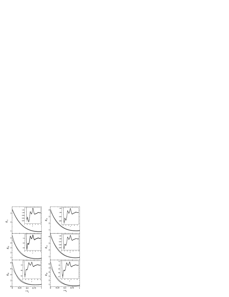
Figure 11: Radial distribution functions $g_{ij}(r)$ for a ternary mixture with diameters $\sigma_{1}=1$, $\sigma_{2}=2$, and $\sigma_{3}=3$ at a packing fraction $\eta=0.49$ with mole fractions $x_{1}=0.7$, $x_{2}=0.2$, and $x_{3}=0.1$. The circles are simulation results MMYSH02 , the solid lines are the RFA predictions, and the dotted lines are the PY predictions.

In Fig. 11 we present a comparison between the results of the RFA method with the PY theory and simulation data MMYSH02 for the RDF of a ternary mixture. In the case of the RFA, we have used the eCS2 contact values and the corresponding isothermal compressibility. The improvement of the RFA over the PY prediction, particularly in the region near contact, is noticeable. Although the RFA accounts nicely for the observed oscillations, it seems to somewhat overestimate the depth of the first minimum.

Explicit knowledge of $G_{ij}(s)$ also allows us to determine the Fourier transform $\widetilde{h}_{ij}(q)$ through the relation

$$\widetilde{h}_{ij}(q)=-2\pi\left.\frac{G_{ij}(s)-G_{ij}(-s)}{s}\right|_{s={\rm i}q}.$$ (161)

The structure factor $S_{ij}(q)$ may be expressed in terms of $\widetilde{h}_{ij}(q)$ as HM86

$$S_{ij}(q)=x_{i}\delta_{ij}+\rho x_{i}x_{j}\widetilde{h}_{ij}(q).$$ (162)

In the particular case of a binary mixture, rather than the individual structure factors $S_{ij}(q)$, it is some combination of them which may be easily associated with fluctuations of the thermodynamic variables AL67 ; BT70 . Specifically, the quantities HM86

$$S_{nn}(q)=S_{11}(q)+S_{22}(q)+2S_{12}(q),$$ (163)

$$S_{nc}(q)=x_{2}S_{11}(q)-x_{1}S_{22}(q)+(x_{2}-x_{1})S_{12}(q),$$ (164)

$$S_{cc}(q)=x_{2}^{2}S_{11}(q)+x_{1}^{2}S_{22}(q)-2x_{1}x_{2}S_{12}(q)$$ (165)

are sometimes required.

After replacement of $\widehat{h}_{ij}(q)=\sqrt{\rho_{i}\rho_{j}}\widetilde{h}_{ij}(q)$ in Eq. (147), one easily gets $\widetilde{c}_{ij}(q)$. Subsequent inverse Fourier transformation yields $c_{ij}(r)$. The result gives $c_{ij}(r)$ for $r>\sigma_{ij}$ as the superposition of $N$ Yukawas YSH00 , namely

$$c_{ij}(r)=\sum_{\ell=1}^{N}K_{ij}^{(\ell)}\frac{\mathrm{e}^{-\kappa_{\ell}r}}{r},$$ (166)

where $q=\pm{\rm i}\kappa_{\ell}$ with $\ell=1,\ldots,N$ are the zeros of $\det\left[{\sf I}+\widehat{\sf h}(q)\right]$ and the amplitudes $K_{ij}^{(\ell)}$ are obtained by applying the residue theorem as

$$K_{ij}^{(\ell)}=\frac{{\rm i}\kappa_{\ell}}{2\pi}\lim_{q\rightarrow{\rm i}\kappa_{\ell}}\widetilde{c}_{ij}(q)(q-{\rm i}\kappa_{\ell}).$$ (167)

The indirect correlation functions $\gamma_{ij}(r)\equiv h_{ij}(r)-c_{ij}(r)$ readily follow from the previous results for the RDF and direct correlation functions. Finally, in this case the bridge functions $B_{ij}(r)$ for $r>\sigma_{ij}$ are linked to $g_{ij}(r)$ and $c_{ij}(r)$ through

$$B_{ij}(r)=\ln g_{ij}(r)-\gamma_{ij}(r)$$ (168)

and so once more we have a full set of analytical results for the structural properties of a multicomponent fluid mixture of HS once the contact values $g_{ij}(\sigma_{ij})$ are specified.

4 Other Related Systems

The philosophy behind the RFA method to derive the structural properties of three-dimensional HS systems can be adapted to deal with other related systems. The main common features of the RFA can be summarized as follows. First, one chooses to represent the RDF in Laplace space. Next, using as a guide the low-density form of the Laplace transform, an auxiliary function is defined which is approximated by a rational or a rational-like form. Finally, the coefficients are determined by imposing some basic consistency conditions. In this section we consider the cases of sticky-hard-sphere, square-well, and hard-disk fluids. In the two former cases the RFA program is followed quite literally, while in the latter case it is done more indirectly through the RFA method as applied to hard rods ($d=1$) and hard spheres ($d=3$).

4.1 Sticky Hard Spheres

The sticky-hard-sphere (SHS) fluid model has received a lot of attention since it was first introduced by Baxter in 1968 B68 and later extended to multicomponent mixtures by Perram and Smith PS75 and, independently, by Barboy BT79 . In this model, the molecular interaction may be defined via square-well (SW) potentials of infinite depth and vanishing width, thus embodying the two essential characteristics of real molecular interactions, namely a harsh repulsion and an attractive part. In spite of their known shortcomings BJG97 , an important feature of SHS systems is that they allow for an exact solution of the OZ equation in the PY approximation B68 ; PS75 . Furthermore, they are thought to be appropriate for describing structural properties of colloidal systems, micelles, and microemulsions, as well as some aspects of gas-liquid equilibrium, ionic fluids and mixtures, solvent mediated forces, adsorption phenomena, polydisperse systems, and fluids containing chainlike molecules BB74 ; varios_SHS ; SG87 ; MF04a ; MF04b .

Let us consider an $N$-component mixture of spherical particles interacting according to the SW potential

$$\phi_{ij}(r)=\left\{\begin{array}[]{ll}\infty,&r<\sigma_{ij},\\ -\epsilon_{ij},&\sigma_{ij}<r<R_{ij},\\ 0,&r>R_{ij}.\end{array}\right.$$ (169)

As in the case of additive HS, $\sigma_{ij}=(\sigma_{i}+\sigma_{j})/2$ is the distance between the centers of a sphere of species $i$ and a sphere of species $j$ at contact. In addition, $\epsilon_{ij}$ is the well depth and $R_{ij}-\sigma_{ij}$ indicates the well width. We now take the SHS limit B68 , namely

$$R_{ij}\to\sigma_{ij},\quad\epsilon_{ij}\to\infty,\quad\tau_{ij}\equiv\frac{1}{12}\frac{\sigma_{ij}}{R_{ij}-\sigma_{ij}}\mathrm{e}^{-\epsilon_{ij}/k_{B}T}=\text{ finite},$$ (170)

where the $\tau_{ij}$ are monotonically increasing functions of the temperature $T$ and their inverses measure the degree of “adhesiveness” of the interacting spheres $i$ and $j$. Even without strictly taking the mathematical limits (170), short-range SW fluids can be well described in practice by the SHS model MYS06 .

The virial EOS for the SHS mixture is given by

$$Z = 1+\frac{1}{6}\rho\sum_{i,j=1}^{N}x_{i}x_{j}\int\mathrm{d}{\bf r}\,ry_{ij}(r)\frac{\mathrm{d}}{\mathrm{d}r}\mathrm{e}^{-\phi_{ij}(r)/k_{B}T}$$ (171)

$$= 1+\frac{2\pi}{3}\rho\sum_{i,j=1}^{N}x_{i}x_{j}\sigma_{ij}^{3}y_{ij}(\sigma_{ij})\left[1-\frac{1}{12\tau_{ij}}\left(3+\frac{y_{ij}^{\prime}(\sigma_{ij})}{y_{ij}(\sigma_{ij})}\right)\right],$$

where $y_{ij}(r)\equiv g_{ij}(r)\mathrm{e}^{\phi_{ij}(r)/k_{B}T}$ is the cavity function and $y_{ij}^{\prime}(r)=\mathrm{d}y_{ij}(r)/\mathrm{d}r$. Since $y_{ij}(r)$ must be continuous, it follows that

$$g_{ij}(r)=y_{ij}(r)\left[\Theta(r-\sigma_{ij})+\frac{\sigma_{ij}}{12\tau_{ij}}\delta(r-\sigma_{ij})\right].$$ (172)

The case of a HS system is recovered by taking the limit of vanishing adhesiveness $\tau_{ij}^{-1}\to 0$, in which case Eq. (171) reduces to the three-dimensional version of Eq. (2). On the other hand, the compressibility EOS, Eq. (145), is valid for any interaction potential, including SHS.

As in the case of HS, it is convenient to define the Laplace transform (149). The condition $y_{ij}(\sigma_{ij})=\text{finite}$ translates into the following large $s$ behavior of $G_{ij}(s)$:

$$\mathrm{e}^{\sigma_{ij}s}G_{ij}(s)=\sigma_{ij}^{2}y_{ij}(\sigma_{ij})\left(\frac{1}{12\tau_{ij}}+\sigma_{ij}^{-1}s^{-1}\right)+{\cal O}(s^{-2}),$$ (173)

which differs from (151): while $\mathrm{e}^{\sigma_{ij}s}G_{ij}(s)\sim s^{-1}$ for HS, $\mathrm{e}^{\sigma_{ij}s}G_{ij}(s)\sim s^{0}$ for SHS. However, the small $s$ behavior is still given by Eq. (152), as a consequence of the condition $\chi^{-1}=\text{finite}$.

The RFA proposal for SHS mixtures SYH98 keeps the form (154), except that now

$$L_{ij}(s)=L_{ij}^{(0)}+L_{ij}^{(1)}s+L_{ij}^{(2)}s^{2}+L_{ij}^{(3)}s^{3},$$ (174)

$$A_{ij}(s)=\rho_{i}\left[\varphi_{2}(\sigma_{i}s)\sigma_{i}^{3}L_{ij}^{(0)}+\varphi_{1}(\sigma_{i}s)\sigma_{i}^{2}L_{ij}^{(1)}+\varphi_{0}(\sigma_{i}s)\sigma_{i}L_{ij}^{(2)}-\mathrm{e}^{-\sigma_{i}s}L_{ij}^{(3)}\right],$$ (175)

instead of Eqs. (155) and (156). By construction, Eqs. (154), (174), and (175) comply with the requirement $\lim_{s\rightarrow\infty}\mathrm{e}^{\sigma_{ij}s}G_{ij}(s)=\text{finite}$. Further, in view of Eq. (152), the coefficients of $s^{0}$ and $s$ in the power series expansion of $s^{2}G_{ij}(s)$ must be 1 and 0, respectively. This yields $2N^{2}$ conditions that allow us to express ${\sf L}^{(0)}$ and ${\sf L}^{(1)}$ in terms of ${\sf L}^{(2)}$, ${\sf L}^{(3)}$, and $\alpha$ as SYH98

$$L_{ij}^{(0)}=\vartheta_{1}+\vartheta_{2}\sigma_{j}+2\vartheta_{2}\alpha-\vartheta_{1}\sum_{k=1}^{N}\rho_{k}\left(\sigma_{k}L_{kj}^{(2)}-L_{kj}^{(3)}\right)-\vartheta_{2}\sum_{k=1}^{N}\rho_{k}\sigma_{k}L_{kj}^{(3)},$$ (176)

$$L_{ij}^{(1)} = \vartheta_{1}\sigma_{ij}+\frac{1}{2}\vartheta_{2}\sigma_{i}\sigma_{j}+(\vartheta_{1}+\vartheta_{2}\sigma_{i})\alpha-\frac{1}{2}\vartheta_{1}\sigma_{i}\sum_{k=1}^{N}\rho_{k}\left(\sigma_{k}L_{kj}^{(2)}-L_{kj}^{(3)}\right)$$ (177)

$$-\frac{1}{2}\left(\vartheta_{1}+\vartheta_{2}\sigma_{i}\right)\sum_{k=1}^{N}\rho_{k}\sigma_{k}L_{kj}^{(3)},$$

where $\vartheta_{1}$ and $\vartheta_{2}$ are defined below Eq. (158). We have the freedom to choose ${\sf L}^{(3)}$ and $\alpha$, but ${\sf L}^{(2)}$ is constrained by the condition (173), i.e., the ratio between the first and second terms in the expansion of $\mathrm{e}^{\sigma_{ij}s}G_{ij}(s)$ for large $s$ must be exactly equal to $\sigma_{ij}/12\tau_{ij}$.

First-Order Approximation (PY Solution)

The simplest approximation consists of making $\alpha=0$. In view of the condition $\mathrm{e}^{\sigma_{ij}s}G_{ij}(s)\sim s^{0}$ for large $s$, this implies $L_{ij}^{(3)}=0$. In that case, the large $s$ behavior that follows from Eq. (154) is

$$2\pi\mathrm{e}^{\sigma_{ij}s}G_{ij}(s)=L_{ij}^{(2)}+\left[L_{ij}^{(1)}+\left({\sf L}^{(2)}\cdot{\sf D}\right)_{ij}\right]s^{-1}+{\cal O}(s^{-2}),$$ (178)

where

$$D_{ij}\equiv\rho_{i}\left(\frac{1}{2}\sigma_{i}^{2}L_{ij}^{(0)}-\sigma_{i}L_{ij}^{(1)}+L_{ij}^{(2)}\right).$$ (179)

Comparison with Eq. (173) yields

$$y_{ij}(\sigma_{ij})=\frac{6\tau_{ij}}{\pi\sigma_{ij}^{2}}L_{ij}^{(2)},$$ (180)

$$\frac{12\tau_{ij}L_{ij}^{(2)}}{\sigma_{ij}}=L_{ij}^{(1)}+\sum_{k=1}^{N}L_{ik}^{(2)}D_{kj}.$$ (181)

Taking into account Eqs. (176) and (177) (with $L_{ij}^{(2)}=L_{ji}^{(2)}$ and of course also with $\alpha=0$ and ${\sf L}^{(3)}=0$), Eq. (181) becomes a closed equation for ${\sf L}^{(2)}$:

$$\frac{12\tau_{ij}L_{ij}^{(2)}}{\sigma_{ij}}=\vartheta_{1}\sigma_{ij}+\frac{1}{2}\vartheta_{2}\sigma_{i}\sigma_{j}-\frac{1}{2}\vartheta_{1}\sum_{k=1}^{N}\rho_{k}\sigma_{k}\left(L_{ki}^{(2)}\sigma_{j}+L_{kj}^{(2)}\sigma_{i}\right)+\sum_{k=1}^{N}\rho_{k}L_{ki}^{(2)}L_{kj}^{(2)}.$$ (182)

The physical root $\mathsf{L}^{(2)}$ of Eq. (182) is the one vanishing in the HS limit $\tau_{ij}\to\infty$. Once known, Eq. (180) gives the contact values.

This first-order approximation obtained from the RFA method turns out to coincide with the exact solution of the PY theory for SHS PS75 .

Second-Order Approximation

As in the case of HS mixtures, a more flexible proposal is obtained by keeping $\alpha$ (and, consequently, $L_{ij}^{(3)}$) different from zero. In that case, instead of Eq. (178), one has

$$2\pi\mathrm{e}^{\sigma_{ij}s}G_{ij}(s)=\frac{L_{ij}^{(3)}}{\alpha}\left[1+\left(\frac{L_{ij}^{(2)}}{L_{ij}^{(3)}}-\frac{1}{\alpha}\right)s^{-1}\right]+{\cal O}(s^{-2}).$$ (183)

This implies

$$L_{ij}^{(3)}=\frac{\pi\sigma_{ij}^{2}}{6\tau_{ij}}\alpha y_{ij}(\sigma_{ij}),$$ (184)

$$\frac{12\tau_{ij}L_{ij}^{(3)}}{\sigma_{ij}}=L_{ij}^{(2)}-\frac{L_{ij}^{(3)}}{\alpha}.$$ (185)

If we fix $y_{ij}(\sigma_{ij})$, Eqs. (176), (177), (184), and (185) allow one to express ${\sf L}^{(0)}$, ${\sf L}^{(1)}$, ${\sf L}^{(2)}$, and ${\sf L}^{(3)}$ as linear functions of $\alpha$. Thus, only the scalar parameter $\alpha$ remains to be fixed, analogously to what happens in the HS case. As done in the latter case, one possibility is to choose $\alpha$ in order to reproduce the isothermal compressibility $\chi$ given by Eq. (148). To do so, one needs to find the coefficients $H_{ij}^{(1)}$ appearing in Eq. (152). The result is SYH98

$${\sf H}^{(0)}={\sf C}^{(0)}\cdot\left(\mathsf{I}-{\sf A}^{(0)}\right)^{-1},$$ (186)

$${\sf H}^{(1)}={\sf C}^{(1)}\cdot\left(\mathsf{I}-{\sf A}^{(0)}\right)^{-1},$$ (187)

where

$$C_{ij}^{(0)}=\frac{1}{2\pi}L_{ij}^{(2)}+\sum_{k=1}^{N}A_{kj}^{(2)}-\sum_{k=1}^{N}\sigma_{ik}\left(\alpha\delta_{kj}-A_{kj}^{(1)}\right)-\sum_{k=1}^{N}\frac{1}{2}\sigma_{ik}^{2}\left(\delta_{kj}-A_{kj}^{(0)}\right),$$ (188)

$$C_{ij}^{(1)} = \frac{1}{2\pi}L_{ij}^{(3)}+\sum_{k=1}^{N}A_{kj}^{(3)}+\sum_{k=1}^{N}\sigma_{ik}A_{kj}^{(2)}-\sum_{k=1}^{N}\left(\frac{1}{2}\sigma_{ik}^{2}+H_{ik}^{(0)}\right)\left(\alpha\delta_{kj}-A_{kj}^{(1)}\right)$$ (189)

$$-\sum_{k=1}^{N}\left(\frac{1}{6}\sigma_{ik}^{3}+\sigma_{ik}H_{ik}^{(0)}\right)\left(\delta_{kj}-A_{kj}^{(0)}\right),$$

$$A_{ij}^{{(n)}}=(-1)^{n}\rho_{i}\left[\frac{\sigma_{i}^{n+3}}{(n+3)!}L_{ij}^{(0)}-\frac{\sigma_{i}^{n+2}}{(n+2)!}L_{ij}^{(1)}+\frac{\sigma_{i}^{n+1}}{(n+1)!}L_{ij}^{(2)}-\frac{\sigma_{i}^{n}}{n!}L_{ij}^{(3)}\right].$$ (190)

Equation (187) gives ${\sf H}^{(1)}$ in terms of $\alpha$: $H_{ij}^{(1)}=P_{ij}(\alpha)/[Q(\alpha)]^{2}$, where $P_{ij}(\alpha)$ denotes a polynomial in $\alpha$ of degree $2N$ and $Q(\alpha)$ denotes a polynomial of degree $N$. It turns out then that, seen as a function of $\alpha$, $\chi$ is the ratio of two polynomials of degree $2N$. Given a value of $\chi$, one may solve for $\alpha$. The physical solution, which has to fulfill the requirement that $G_{ij}(s)$ is positive definite for positive real $s$, corresponds to the smallest positive real root.

Once $\alpha$ is known, the scheme is complete: Eq. (184) gives ${\sf L}^{(3)}$, then ${\sf L}^{(2)}$ is obtained from Eq. (185), and finally ${\sf L}^{(1)}$ and ${\sf L}^{(0)}$ are given by Eqs. (176) and (177), respectively. Explicit knowledge of $G_{ij}(s)$ through Eqs. (154), (174), and (175) allows one to determine the Fourier transform $\widetilde{h}_{ij}(q)$ and the structure factor $S_{ij}(q)$ through Eqs.  (161) and (162), respectively. Finally, inverse Laplace transformation of $G_{ij}(s)$ yields $g_{ij}(r)$ notebook .

Single Component SHS Fluids

The special case of single component SHS fluids YS93b ; YS93c can be obtained from the multicomponent one by taking $\sigma_{ij}=\sigma$ and $\tau_{ij}=\tau$. Thus, the Laplace transform of $rg(r)$ in the RFA is

$$G(s)=\frac{\mathrm{e}^{-s}}{2\pi s^{2}}\frac{L^{(0)}+L^{(1)}s+{L^{(2)}}s^{2}+L^{(3)}s^{3}}{1+\alpha s-\rho\left[\varphi_{2}(s)L^{(0)}+\varphi_{1}(s)L^{(1)}+\varphi_{0}(s)L^{(2)}-\mathrm{e}^{-s}L^{(3)}\right]},$$ (191)

where we have taken $\sigma=1$. Equations (176) and (177) become

$$L^{(0)}=2\pi\frac{1+2\eta}{(1-\eta)^{2}}+\frac{12\eta}{1-\eta}\left(\frac{\pi\alpha}{1-\eta}-{L^{(2)}}\right)+\frac{12\eta}{(1-\eta)^{2}}(1-4\eta)L^{(3)},$$ (192)

$$L^{(1)}=2\pi\frac{1+\frac{1}{2}\eta}{(1-\eta)^{2}}+\frac{2}{1-\eta}\left(\pi\frac{1+2\eta}{1-\eta}\alpha-3\eta{L^{(2)}}\right)-\frac{18\eta^{2}}{(1-\eta)^{2}}L^{(3)}.$$ (193)

The choice $\alpha=L^{(3)}=0$ makes Eq. (191) coincide with the exact solution to the PY approximation for SHS B68 , where $L^{(2)}$ is the physical root (i.e., the one vanishing in the limit $\tau\to\infty$) of the quadratic equation [see Eq. (182)]

$$12\tau L^{(2)}=2\pi\frac{1+2\eta}{(1-\eta)^{2}}-\frac{12\eta}{1-\eta}L^{(2)}+\frac{6}{\pi}\eta{L^{(2)}}^{2}.$$ (194)

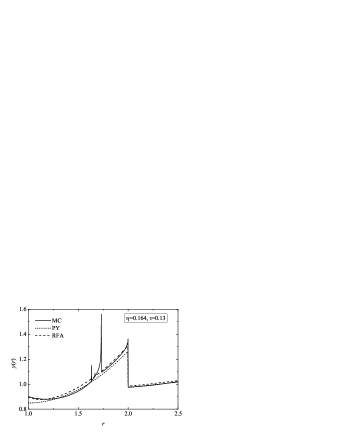
Figure 12: Cavity function of a single component SHS fluid for $\eta=0.164$ and $\tau=0.13$. The solid line represents simulation data MF04a . The dotted and dashed lines represent the PY and RFA approaches, respectively.

We can go beyond the PY approximation by prescribing a contact value $y(1)$, so that, according to Eqs. (184) and (185),

$$L^{(3)}=\frac{\pi}{6}\frac{\alpha}{\tau}y(1),$$ (195)

$$L^{(2)}=\left(12\tau+\frac{1}{\alpha}\right)L^{(3)}.$$ (196)

By prescribing the isothermal compressibility $\chi$, the parameter $\alpha$ can be obtained as the physical solution (namely, the one remaining finite in the limit $\tau\to\infty$) of a quadratic equation YS93c . Thus, given an EOS for the SHS fluid, one can get the thermodynamically consistent values of $y(1)$ and $\chi$ and determine from them all the coefficients appearing in Eq. (191).

Figure 12 shows the cavity function for $\eta=0.164$ and $\tau=0.13$ as obtained from Monte Carlo simulations MF04a and as predicted by the PY and RFA theories, the latter making use of the EOS recently proposed by Miller and Frenkel MF04b . It can be observed that the RFA is not only more accurate than the PY approximation near $r=1$ but also near $r=2$. On the other hand, none of these two approximations account for the singularities (delta-peaks and/or discontinuities) of $y(r)$ at $r=\sqrt{{8}/{3}},{5}/{3},\sqrt{3},2,\ldots$ SG87 ; MF04a .

4.2 Single Component Square-Well Fluids

Now we consider again the SW interaction potential (169) but for a single fluid, i.e., $\sigma_{ij}=\sigma$, $\epsilon_{ij}=\epsilon$, $R_{ij}=R$. Since no exact solution of the PY theory for the SW potential is known, the application of the RFA method is more challenging in this case than for HS and SHS fluids.

As in the cases of HS and SHS, the key quantity is the Laplace transform of $rg(r)$ defined by Eq. (98). It is again convenient to introduce the auxiliary function $\Psi(s)$ through Eq. (99). As before, the conditions $g(r)=\text{finite}$ and $\chi=\text{finite}$ imply Eqs. (102) and (104), respectively. However, the important difference between HS and SHS fluids is that in the latter case $G(s)$ must reflect the fact that $g(r)$ is discontinuous at $r=R$ as a consequence of the discontinuity of the potential $\phi(r)$ and the continuity of the cavity function $y(r)$. This implies that $G(s)$, and hence $\Psi(s)$, must contain the exponential term $\mathrm{e}^{-(R-\sigma)s}$. This manifests itself in the low-density limit, where the condition $\lim_{\rho\to 0}y(r)=1$ yields

$$\lim_{\rho\to 0}\Psi(s)=\frac{1}{2\pi}\frac{s^{3}}{\mathrm{e}^{1/T^{*}}(1+s)-\mathrm{e}^{-(R-1)s}(\mathrm{e}^{1/T^{*}}-1)(1+Rs)},$$ (197)

where $T^{*}\equiv k_{B}T/\epsilon$ and we have taken $\sigma=1$.

In the spirit of the RFA method, the simplest form that complies with Eq. (102) and is consistent with Eq. (197) is YS94

$$\Psi(s)=\frac{1}{2\pi}\frac{-12\eta+E_{1}s+E_{2}s^{2}+E_{3}s^{3}}{1+Q_{0}+Q_{1}s-\mathrm{e}^{-(R-1)s}\left(Q_{0}+Q_{2}s\right)},$$ (198)

where the coefficients $Q_{0}$, $Q_{1}$, $Q_{2}$, $E_{1}$, $E_{2}$, and $E_{3}$ are functions of $\eta$, $T^{*}$, and $R$. The condition (104) allows one to express the parameters $Q_{1}$, $E_{1}$, $E_{2}$, and $E_{3}$ as linear functions of $Q_{0}$ and $Q_{2}$ YS94 ; AS01 :

$$Q_{1} = \frac{1}{1+2\eta}\left[1+\frac{\eta}{2}+2\eta(R^{3}-1)Q_{2}-\frac{\eta}{2}(R-1)^{2}(R^{2}+2R+3){Q_{0}}\right]$$ (199)

$$+Q_{2}-(R-1)Q_{0},$$

$$E_{1}=\frac{6\eta^{2}}{1+2\eta}\left[{3}-4(R^{3}-1)Q_{2}+(R-1)^{2}(R^{2}+2R+3){Q_{0}}\right],$$ (200)

$$E_{2} = \frac{6\eta}{1+2\eta}\left\{1-\eta-2(R-1)\left[1-2\eta R(R+1)\right]Q_{2}\right.$$ (201)

$$\left.+(R-1)^{2}\left[(1-\eta(R+1)^{2}\right]{Q_{0}}\right\},$$

$$E_{3} = \frac{1}{1+2\eta}\left\{(1-\eta)^{2}+6\eta(R-1)\left(R+1-2\eta R^{2}\right)Q_{2}\right.$$ (202)

$$\left.-\eta(R-1)^{2}[4+2R-\eta(3R^{2}+2R+1)]{Q_{0}}\right\}.$$

From Eq. (102), we have

$$g(1^{+})=\frac{Q_{1}}{E_{3}}.$$ (203)

The complete RDF is given by Eq. (122), where now Eq. (198) must be used in Eq. (123). In particular, $\psi_{1}(r)$ and $\psi_{2}(r)$ are

$$\psi_{1}(r)=\psi_{10}(r)\Theta(r)+\psi_{11}(r+1-R)\Theta(r+1-R),$$ (204)

$$\psi_{2}(r)=\psi_{20}(r)\Theta(r)+\psi_{21}(r+1-R)\Theta(r+1-R)+\psi_{22}(r+2-2R)\Theta(r+2-2R),$$ (205)

where

$$\psi_{1k}(r)={2\pi}\sum_{i=1}^{3}\frac{W_{1k}(s_{i})}{E^{\prime}(s_{i})}s_{i}\mathrm{e}^{s_{i}x},$$ (206)

$$\psi_{2k}(r)=-4\pi^{2}\sum_{i=1}^{3}\left[rW_{2k}(s_{i})+W_{2k}^{\prime}(s_{i})-W_{2k}(s_{i})\frac{E^{\prime\prime}(s_{i})}{E^{\prime}(s_{i})}\right]\frac{\mathrm{e}^{s_{i}r}}{[E^{\prime}(s_{i})]^{2}}.$$ (207)

Here, $s_{i}$ are the three distinct roots of $E(s)\equiv-12\eta+E_{1}s+E_{2}s^{2}+E_{3}s^{3}$ and

$$W_{10}(s)\equiv 1+Q_{0}+Q_{1}s,\quad W_{11}(s)\equiv-(Q_{0}+Q_{2}s).$$ (208)

$$W_{20}(s)\equiv s[W_{10}(s)]^{2},\quad W_{21}(s)\equiv 2sW_{10}(s)W_{11}(s),\quad W_{22}(s)\equiv s[W_{11}(s)]^{2}.$$ (209)

Figure 13: Radial distribution function of a single component SW fluid for $R=1.05$, $\rho\sigma^{3}=0.8$, and $T^{*}=0.5$ (top panel), for $R=1.5$, $\rho\sigma^{3}=0.4$, and $T^{*}=1.5$ (middle panel), and for $R=2.0$, $\rho\sigma^{3}=0.4$, and $T^{*}=3.0$ (bottom panel). The circles represent simulation data LSYS05 and the solid lines refer to the results obtained from the RFA method.

To close the proposal, we need to determine the parameters $Q_{0}$ and $Q_{2}$ by imposing two new conditions. An obvious condition is the continuity of the cavity function at $r=R$, what implies

$$g(R^{+})=e^{1/T^{*}}g(R^{-}).$$ (210)

This yields

$$\left(1-e^{-1/T^{*}}\right)\psi_{10}(R-1)=-\psi_{11}(0)=2\pi\frac{Q_{2}}{E_{3}}.$$ (211)

As an extra condition, we could enforce the continuity of the first derivative $y^{\prime}(r)$ at $r=R$ A00 . However, this complicates the problem too much without any relevant gain in accuracy. In principle, it might be possible to impose consistency with a given EOS, via either the virial route, the compressibility route, or the energy route. But this is not practical since no simple EOS for SW fluids is at our disposal for wide values of density, temperature, and range. As a compromise between simplicity and accuracy, we fix the parameter $Q_{0}$ at its exact zero-density limit value, namely $Q_{0}=e^{1/T^{*}}-1$ YS94 . Therefore, Eq. (211) becomes a transcendental equation for $Q_{2}$ that needs to be solved numerically. For narrow SW potentials, however, it is possible to replace the exact condition (210) by a simpler one allowing $Q_{2}$ to be obtained analytically AS01 , which is especially useful for determining the thermodynamic properties AS01 ; LSAS03 .

It can be proven that the RFA proposal (198) reduces to the exact solutions of the PY equation W63 ; B68 in the HS limit, i.e., $\epsilon\to 0$ or $R\to 1$, and in the SHS limit, i.e., $\epsilon\to\infty$ and $R\to 1$ with $(R-1)\mathrm{e}^{1/T^{*}}=\text{finite}$ YS94 ; AS01 .

Comparison with computer simulations YS94 ; AS01 ; LSAS03 ; LSYS05 shows that the RFA for SW fluids is rather accurate at any fluid density if the potential well is sufficiently narrow (say $R\leq 1.2$), as well as for any width if the density is small enough (say $\rho\sigma^{3}\leq 0.4$). However, as the width and/or the density increase, the RFA predictions worsen, especially at low temperatures. As an illustration, Fig. 13 compares the RDF provided by the RFA with Monte Carlo data LSYS05 for three representative cases.

4.3 Hard Disks

As is well known, the PY theory is exactly solvable for HS fluids with an odd number of dimensions FI81 ; L84 ; RHS04 . In particular, in the case of hard rods ($d=1$), the PY theory provides the exact RDF $g(r)$ or, equivalently, the exact cavity function $y(r)$ outside the hard core (i.e., for $r>\sigma$). However, it does not reproduce the exact $y(r)$ in the overlapping region (i.e., for $r<\sigma$) MS06 . The full exact one-dimensional cavity function is MS06

$$y_{\text{HR}}(r|\eta)=\frac{\mathrm{e}^{-(r-1)\eta/(1-\eta)}}{1-\eta}+\sum_{n=2}^{\infty}\frac{\eta^{n-1}\mathrm{e}^{-(r-n)\eta/(1-\eta)}}{(1-\eta)^{n}(n-1)!}(r-n)^{n-1}\Theta(r-n),$$ (212)

where the subscript HR stands for hard rods and, as usual, $\sigma=1$ has been taken. Consequently, one has

$$g_{\text{HR}}(1^{+}|\eta)=\frac{1}{1-\eta},\quad\int_{0}^{\infty}dr\,rh_{\text{HR}}(r|\eta)\equiv H_{\text{HR}}^{(0)}(\eta)=-\frac{1}{2}+\frac{2}{3}\eta-\frac{1}{4}\eta^{2}.$$ (213)

When $d$ is even, the PY equation is not analytically solvable for the HS interaction. In particular, in the important case of hard disks ($d=2$), one must resort to numerical solutions of the PY equation BH76 ; CRR76 . Alternatively, a simple heuristic approach has proven to yield reasonably good results YS93a . Such an approach is based on the naïve assumption that the structure and spatial correlations of a hard-disk fluid share some features with those of a hard-rod and a hard-sphere fluid. This fuzzy idea becomes a more specific one by means of the following simple model YS93a :

$$g_{\text{HD}}(r|\eta)=\nu(\eta)g_{\text{HR}}(r|\omega_{1}(\eta)\eta)+[1-\nu(\eta)]g_{\text{HS}}(r|\omega_{3}(\eta)\eta).$$ (214)

Here, the subscript HD stands for hard disks ($d=2$) and the subscript HS stands for hard spheres ($d=3$). The parameter $\nu(\eta)$ is a density-dependent mixing parameter, while $\omega_{1}(\eta)\eta$ and $\omega_{3}(\eta)\eta$ are the packing fractions in one and three dimensions, respectively, which are “equivalent” to the packing fraction $\eta$ in two dimensions. In Eq. (214), it is natural to take for $g_{\text{HR}}(r|\eta)$ the exact solution, Eq. (212). As for $g_{\text{HR}}(r|\eta)$, one might use the RFA recipe described in Section 3. However, in order to keep the model (214) as simple as possible, it is sufficient for practical purposes to take the PY solution, Eq. (108). In the latter approximation,

$$g_{\text{HS}}(1^{+}|\eta)=\frac{1+\eta/2}{(1-\eta)^{2}},\quad\int_{0}^{\infty}\mathrm{d}r\,rh_{\text{HS}}(r|\eta)\equiv H_{\text{HS}}^{(0)}(\eta)=-\frac{10-2\eta+\eta^{2}}{20(1+2\eta)}.$$ (215)

In order to close the model (214), we still need to determine the parameters $\nu(\eta)$, $\omega_{1}(\eta)$, and $\omega_{3}(\eta)$. To that end, we first impose the condition that Eq. (214) must be consistent with a prescribed contact value $g_{\text{HD}}(1^{+}|\eta)$ or, equivalently, with a prescribed compressibility factor $Z_{\text{HD}}(\eta)=1+2\eta g_{\text{HD}}(1^{+}|\eta)$, with independence of the choice of the mixing parameter $\nu(\eta)$. In other words,

$$g_{\text{HD}}(1^{+}|\eta)=g_{\text{HR}}(1^{+}|\omega_{1}(\eta)\eta)=g_{\text{HS}}(1^{+}|\omega_{3}(\eta)\eta).$$ (216)

Making use of Eqs. (213) and (215), this yields

$$\omega_{1}(\eta)=\frac{g_{\text{HD}}(1^{+}|\eta)-1}{\eta g_{\text{HD}}(1^{+}|\eta)},\quad\omega_{3}(\eta)=\frac{4g_{\text{HD}}(1^{+}|\eta)+1-\sqrt{24g_{\text{HD}}(1^{+}|\eta)+1}}{4\eta g_{\text{HD}}(1^{+}|\eta)}.$$ (217)

Once $\omega_{1}(\eta)$ and $\omega_{3}(\eta)$ are known, we can determine $\nu(\eta)$ by imposing that the model (214) reproduces the isothermal compressibility $\chi_{\text{HD}}(\eta)$ thermodynamically consistent with the prescribed $Z_{\text{HD}}(\eta)$ [cf. Eq. (97)]. From Eqs. (96) and (214) one has

$$\chi_{\text{HD}}(\eta)=1+8\eta\int_{0}^{\infty}\mathrm{d}r\,r\left\{\nu(\eta)h_{\text{HR}}(r|\omega_{1}(\eta)\eta)+\left[1-\nu(\eta)\right]h_{\text{HS}}(r|\omega_{3}(\eta)\eta)\right\},$$ (218)

so that

$$\nu(\eta)=\frac{\left[\chi_{\text{HD}}(\eta)-1\right]/8\eta-H_{\text{HS}}^{(0)}(\omega_{3}(\eta)\eta)}{H_{\text{HR}}^{(0)}(\omega_{1}(\eta)\eta)-H_{\text{HS}}^{(0)}(\omega_{3}(\eta)\eta)},$$ (219)

where $H_{\text{HR}}^{(0)}(\eta)$ and $H_{\text{HS}}^{(0)}(\eta)$ are given by Eqs. (213) and (215), respectively.

Once a sensible EOS for hard disks is chosen [see, for instance, Table 1], Eqs. (217) and (219) provide the parameters of the model (214). The results show that the scaling factor $\omega_{1}(\eta)$ is a decreasing function, while $\omega_{3}(\eta)$ is an increasing function YS93a . As for the mixing parameter $\nu(\eta)$, it is hardly dependent of density and takes values around $\nu(\eta)\simeq 0.35$–0.40.

Comparison of the interpolation model (214) with computer simulation results shows a surprisingly good agreement, despite the crudeness of the model and the absence of empirical fitting parameters, especially at low and moderate densities YS93a . The discrepancies become important only for distances beyond the location of the second peak and for densities close to the stability threshold.

5 Perturbation Theory

When one wants to deal with realistic intermolecular interactions, the problem of deriving the thermodynamic and structural properties of the system becomes rather formidable. Thus, perturbation theories of liquids have been devised since the mid twentieth century. In the case of single component fluids, the use of an accurate and well characterized RDF for the HS fluid in a perturbation theory opens up the possibility of deriving a closed theoretical scheme for the determination of the thermodynamic and structural properties of more realistic models, such as the Lennard–Jones (LJ) fluid. In this section, we will consider this model system, which captures the basic physical properties of real non-polar fluids, to illustrate the procedure.

In the application of the perturbation theory of liquids, the stepping stone has been the use of the HS RDF obtained from the solution to the PY equation. Unfortunately, the absence of thermodynamic consistency present in the PY approximation (as well as in other integral equation theories) may clearly contaminate the results derived from its use within a perturbative treatment. In what follows we will reanalyze the different theoretical schemes for the thermodynamics of LJ fluids that have been constructed with perturbation theory, taking as the reference system the HS fluid. This includes the consideration of the RDF as obtained with the RFA method, which embodies thermodynamic consistency, as well as the proposal of a unifying framework in which all schemes fit in. With our development, we will be able to present a formulation which lends itself to relatively easy numerical calculations while retaining the merits that analytical results provide, namely a detailed knowledge and control of all the approximations involved.

Let us consider a three-dimensional fluid system defined by a pair interaction potential $\phi(r)$. The virial and energy EOS express the compressibility factor $Z$ and the excess part of the Helmholtz free energy per unit volume $f^{\text{ex}}$, respectively, in terms of the RDF of the system as

$$Z=1-\frac{2}{3}\pi\rho\beta\int_{0}^{\infty}\mathrm{d}r\,\frac{\partial\phi(r)}{\partial r}g(r)r^{3},$$ (220)

$$\frac{f^{\text{ex}}}{\rho k_{B}T}=2\pi\rho\beta\int_{0}^{\infty}\mathrm{d}r\,\phi(r)g(r)r^{2},$$ (221)

where $\beta\equiv 1/k_{B}T$. Let us now assume that $\phi(r)$ is split into a known (reference) part $\phi_{0}(r)$ and a perturbation part $\phi_{1}(r)$. The usual perturbative expansion for the Helmholtz free energy to first order in $\beta$ leads to M76

$$\frac{f}{\rho k_{B}T}=\frac{f_{0}}{\rho k_{B}T}+2\pi\rho\beta\int_{0}^{\infty}\mathrm{d}r\,\phi_{1}(r)g_{0}(r)r^{2}+\mathcal{O}\left(\beta^{2}\right),$$ (222)

where $f_{0}$ and $g_{0}(r)$ are the free energy and the RDF of the reference system, respectively.

The LJ potential is

$$\phi_{\text{LJ}}(r)=4\epsilon\left(r^{-12}-r^{-6}\right),$$ (223)

where $\epsilon$ is the depth of the well and, for simplicity, we have taken the distance at which the potential vanishes as the length unit, i.e., $\phi_{\text{LJ}}(r=1)=0$. For this potential the reference system may be forced to be a HS system, i.e., one can set

$$\phi_{0}(r)=\phi_{\text{HS}}(r)=\left\{\begin{array}[]{ll}\infty,&r\leq\sigma_{0},\\ 0,&r>\sigma_{0},\end{array}\right.$$ (224)

where $\sigma_{0}$ is a conveniently chosen effective HS diameter. In this case the Helmholtz free energy to this order is approximated by

$$\frac{f_{\text{LJ}}}{\rho k_{B}T}\approx\frac{f_{\text{HS}}}{\rho k_{B}T}+2\pi\rho\beta\int_{\sigma_{0}}^{\infty}\mathrm{d}r\,\phi_{\text{LJ}}(r)g_{\text{HS}}({r}/{\sigma_{0}})r^{2}.$$ (225)

Note that Eq. (225) may be rewritten in terms of the Laplace transform $G(s)$ of $(r/\sigma_{0})g_{\text{HS}}({r}/{\sigma_{0}})$ as

$$\frac{f_{\text{LJ}}}{\rho k_{B}T}\approx\frac{f_{\text{HS}}}{\rho k_{B}T}+2\pi\rho\beta\sigma_{0}^{3}\int_{0}^{\infty}\mathrm{d}s\,\Phi_{\text{LJ}}(s)G(s),$$ (226)

where $\Phi_{\text{LJ}}(s)$ satisfies

$$r\phi_{\text{LJ}}(r)=\sigma_{0}\int_{0}^{\infty}\mathrm{d}s\,\mathrm{e}^{-rs/\sigma_{0}}\Phi_{\text{LJ}}(s),$$ (227)

so that

$$\Phi_{\text{LJ}}(s)=4\epsilon\sigma_{0}^{-2}\left[\frac{(s/\sigma_{0})^{10}}{10!}-\frac{(s/\sigma_{0})^{4}}{4!}\right].$$ (228)

Irrespective of the value of the diameter $\sigma_{0}$ of the reference system, the right hand side of Eq. (226) represents always an upper bound for the value of the free energy of the real system. Therefore, it is natural to determine $\sigma_{0}$ so as to provide the least upper bound. This is precisely the variational scheme of Mansoori and Canfield MC69 ; MPC69 and Rasaiah and Stell RS70 , usually referred to as MC/RS, and originally implemented with the PY theory for $G(s)$, Eq. (108). In our case, however, we will consider $G(s)$ as given by the RFA method, Eq. (113). Therefore, at fixed $\rho$ and $\beta$, the effective diameter $\sigma_{0}$ in the MC/RS scheme is obtained from the conditions

$$\frac{\partial}{\partial\sigma_{0}}\left\{\int_{0}^{\eta_{0}}\mathrm{d}\eta\,\frac{Z_{\text{HS}}(\eta)-1}{\eta}\right. + 48\beta\epsilon\sigma_{0}^{-2}\int_{0}^{\infty}\mathrm{d}s\,G(s|\eta_{0})$$ (229)

$$\left.\times\left[\frac{(s/\sigma_{0})^{10}}{10!}-\frac{(s/\sigma_{0})^{4}}{4!}\right]\right\}=0,$$

$$\frac{\partial^{2}}{\partial\sigma_{0}^{2}}\left\{\int_{0}^{\eta_{0}}\mathrm{d}\eta\,\frac{Z_{\text{HS}}(\eta)-1}{\eta}\right. + 48\beta\epsilon\sigma_{0}^{-2}\int_{0}^{\infty}\mathrm{d}s\,G(s|\eta_{0})$$ (230)

$$\left.\times\left[\frac{(s/\sigma_{0})^{10}}{10!}-\frac{(s/\sigma_{0})^{4}}{4!}\right]\right\}>0.$$

In these equations, use has been made of the thermodynamic relationship between the free energy and the compressibility factor, Eq. (78). Moreover, we have called $\eta_{0}\equiv(\pi/6)\rho\sigma_{0}^{3}$ and have made explicit with the notation $G(s|\eta_{0})$ the fact that the HS RDF depends on the packing fraction $\eta_{0}$.

Even if the reference system is not forced to be a HS fluid, one can still use Eq. (226) provided an adequate choice for $\sigma_{0}$ is made such that the expansion involved in the right hand side of Eq. (222) yields the right hand side of Eq. (226) to order $\beta^{2}$. This is the idea of the Barker and Henderson BH67 first order perturbation scheme (BH₁), where the effective HS diameter is

$$\sigma_{0}=\int_{0}^{\infty}\mathrm{d}r\,\left[1-\mathrm{e}^{-\beta\phi_{\text{LJ}}\left(r\right)}\right].$$ (231)

The same ideas may be carried out to higher order in the perturbation expansion. The inclusion of the second order term in the expansion yields the so-called macroscopic compressibility approximation M76 for the free energy, namely

$$\frac{f_{\text{LJ}}}{\rho k_{B}T} = \frac{f_{0}}{\rho k_{B}T}+2\pi\rho\beta\int_{0}^{\infty}\mathrm{d}r\,\phi_{1}(r)g_{0}(r)r^{2}$$ (232)

$$-\pi\rho\beta^{2}\chi_{0}\int_{0}^{\infty}\mathrm{d}r\,\phi_{1}^{2}(r)g_{0}(r)r^{2}+\mathcal{O}\left(\beta^{3}\right),$$

where $\chi_{0}$ is the (reduced) isothermal compressibility of the reference system note .

To implement a particular perturbation scheme in this approximation under a unifying framework that eventually leads to easy numerical evaluation, two further assumptions may prove convenient. First, the perturbation potential $\phi_{1}(r)\equiv\phi_{\text{LJ}}(r)-\phi_{0}(r)$ may be split into two parts using some “molecular size” parameter $\xi\geq\sigma_{0}$ such that

$$\phi_{1}(r)=\left\{\begin{array}[]{ll}\phi_{1a}(r),&0\leq r\leq\xi,\\ \phi_{1b}(r),&r>\xi.\end{array}\right.$$ (233)

Next, a choice for the RDF for the reference system is done in the form

$$g_{0}\left(r\right)\approx\theta(r)y_{\text{HS}}(r/\sigma_{0}),$$ (234)

where $y_{\text{HS}}$ is the cavity (background) correlation function of the HS system and $\theta(r)$ is a step function defined by

$$\theta(r)=\left\{\begin{array}[]{ll}\theta_{a}(r),&0\leq r\leq\xi,\\ \theta_{b}(r),&r>\xi,\end{array}\right.$$ (235)

in which the functions $\theta_{a}(r)$ and $\theta_{b}(r)$ depend on the scheme.

With these assumptions the integrals involved in Eq. (232) may be rewritten as

$$I_{n} \equiv \int_{0}^{\infty}\mathrm{d}r\,\phi_{1}^{n}(r)g_{0}(r)r^{2}$$ (236)

$$= \int_{0}^{\sigma_{0}}\mathrm{d}r\,\phi_{1a}^{n}(r)\theta_{a}(r)y_{\text{HS}}(r/\sigma_{0})r^{2}+\int_{\sigma_{0}}^{\xi}\mathrm{d}r\,\phi_{1a}^{n}(r)\theta_{a}(r)g_{\text{HS}}(r/\sigma_{0})r^{2}$$

$$+\int_{\xi}^{\infty}\mathrm{d}r\,\phi_{1b}^{n}(r)\theta_{b}(r)g_{\text{HS}}(r/\sigma_{0})r^{2},$$

with $n=1,2$ and where the fact that $y_{\text{HS}}(r/\sigma_{0})=g_{\text{HS}}(r/\sigma_{0})$ when $r>\sigma_{0}$ has been used. Decomposing the last integral as $\int_{\xi}^{\infty}=\int_{\sigma_{0}}^{\infty}-\int_{\sigma_{0}}^{\xi}$ and applying the same step as in Eq. (226), Eq. (236) becomes

$$I_{n} = \sigma_{0}^{3}\int_{0}^{\infty}\mathrm{d}s\,\Phi_{nb}(s)G(s)+\int_{0}^{\sigma_{0}}\mathrm{d}r\,\phi_{1a}^{n}(r)\theta_{a}(r)y_{\text{HS}}(r/\sigma_{0})r^{2}$$ (237)

$$+\int_{\sigma_{0}}^{\xi}\mathrm{d}r\,\left[\phi_{1a}^{n}(r)\theta_{a}(r)-\phi_{1b}^{n}(r)\theta_{b}(r)\right]g_{\text{HS}}(r/\sigma_{0})r^{2},$$

where the functions $\Phi_{1b}(s)$ and $\Phi_{2b}(s)$ are defined by the relation

$${r}\phi_{1b}^{n}(r)\theta_{b}(r)=\sigma_{0}\int_{0}^{\infty}\mathrm{d}s\,\mathrm{e}^{-rs/\sigma_{0}}\Phi_{nb}(s).$$ (238)

In the Barker–Henderson second order perturbation scheme (BH₂), one takes

$$\theta_{a}(r)=0,\quad\theta_{b}(r)=1,\quad\xi=\sigma_{0},\quad\phi_{1a}(r)=0,\quad\phi_{1b}(r)=4\epsilon\left({r^{-12}}-{r^{-6}}\right),$$ (239)

and $\sigma_{0}$ is computed according to Eq. (231). This choice ensures that

$$\frac{f_{\text{LJ}}}{\rho k_{B}T} = \frac{f_{\text{HS}}}{\rho k_{B}T}+2\pi\rho\beta\int_{\sigma_{0}}^{\infty}\mathrm{d}r\,\phi_{1}(r)g_{\text{HS}}(r/\sigma_{0})r^{2}$$ (240)

$$-\pi\rho\beta^{2}\chi_{\text{HS}}\int_{\sigma_{0}}^{\infty}\mathrm{d}r\,\phi_{1}^{2}(r)g_{\text{HS}}(r/\sigma_{0})r^{2}+O\left(\beta^{3}\right).$$

On the other hand, if one chooses

$$\theta_{a}(r)=\exp\left[-\beta\left(\phi_{\text{LJ}}(r)+\epsilon\right)\right],\quad\theta_{b}(r)=1,\quad\xi=2^{1/6},$$ (241)

$$\phi_{1a}(r)=-\epsilon,\quad\phi_{1b}(r)=4\epsilon\left({r^{-12}}-{r^{-6}}\right),$$ (242)

the scheme leads to the Weeks–Chandler–Andersen (WCA) theory WCA71 if one determines the HS diameter through the condition $\chi_{0}=\chi_{\text{HS}}$ VW72 , which in turn implies

$$\int_{0}^{\sigma_{0}}\mathrm{d}r\,r^{2}\mathrm{e}^{-\beta\phi_{0}(r)}y_{\text{HS}}(r/\sigma_{0})=\int_{\sigma_{0}}^{2^{1/6}}\mathrm{d}r\,r^{2}g_{\text{HS}}(r/\sigma_{0})\left[1-\mathrm{e}^{-\beta\phi_{0}(r)}\right].$$ (243)

To close the scheme, the HS cavity function has to be provided in the range $0\leq r\leq\sigma_{0}$. Fortunately, relatively simple expressions for $y_{\text{HS}}(r/\sigma_{0})$ are available in the literature HG75 ; BS85 ; ZS88 , apart from our own proposal, Eq. (140).

Note that $\theta_{b}(r)$ and $\phi_{1b}(r)$, and thus also $\Phi_{nb}(s)$, are the same functions in the BH₂ and WCA schemes. It is convenient, in order to have all the quantities needed to evaluate $f_{\text{LJ}}$ in these schemes, to provide explicit expressions for $\Phi_{1b}(s)$ and $\Phi_{2b}(s)$. These are given by [cf. Eq. (228)]

$$\Phi_{1b}(s)=\Phi_{\text{LJ}}(s),$$ (244)

$$\Phi_{2b}(s)=16\epsilon^{2}\sigma_{0}^{-2}\left[\frac{(s/\sigma_{0})^{22}}{22!}-2\frac{(s/\sigma_{0})^{16}}{16!}+\frac{(s/\sigma_{0})^{10}}{10!}\right].$$ (245)

Up to this point, we have embodied the most popular perturbation schemes within a unified framework that requires as input only the EOS of the HS fluid in order to compute the Helmholtz free energy of the LJ system and leads to relatively easy numerical computations. It should be clear that a variety of other possible schemes, requiring the same little input, fit in our unified framework, which is based on the RFA method for $g_{\text{HS}}(r/\sigma_{0})$ and $G(s)$. Once $f_{\text{LJ}}$ has been determined, the compressibility factor of the LJ fluid at a given order of the perturbation expansion readily follows from Eqs. (222) or (232) through the thermodynamic relation

$$Z_{\text{LJ}}=\rho\left(\frac{\partial}{\partial\rho}\frac{f_{\text{LJ}}}{\rho k_{B}T}\right)_{T}.$$ (246)

Taking into account that the HS fluid presents a fluid-solid transition at a freezing packing fraction $\eta_{\text{f}}\simeq 0.494$ HV69 and a solid-fluid transition at a melting packing fraction $\eta_{\text{m}}\simeq 0.54$ HV69 , the fluid-solid and solid-fluid coexistence lines for the LJ system may be computed from the values $(\rho,T)$ determined from the conditions $({\pi}/{6})\rho\sigma_{0}^{3}(\rho,T)=\eta_{\text{f}}$ and $({\pi}/{6})\rho\sigma_{0}^{3}(\rho,T)=\eta_{\text{m}}$, respectively, with the effective diameter $\sigma_{0}(\rho,T)$ obtained using any of the perturbative schemes. Similarly, admitting that there is a glass transition in the HS fluid at the packing fraction $\eta_{\text{g}}\simeq 0.56$ S94 , one can now determine the location of the liquid-glass transition line for the LJ fluid in the $(\rho,T)$ plane from the simple relationship $({\pi}/{6})\rho\sigma_{0}^{3}(\rho,T)=\eta_{\text{g}}$. With a proper choice for $Z_{\text{HS}}$, it has been shown RH03 ; RH01 ; HR04 that the critical point, the structure, and the phase diagram (including a glass transition) of the LJ fluid may be adequately described with this approach.

6 Perspectives

In this chapter we have given a self-contained account of a simple (mostly analytical) framework for the study of the thermodynamic and structural properties of hard-core systems. Whenever possible, the developments have attempted to cater for mixtures with an arbitrary number of components (including polydisperse systems) and arbitrary dimensionality. We started considering the contact values of the RDF because they enter directly into the EOS and are required as input in the RFA method to compute the structural properties. With the aid of consistency conditions, we were able to devise various approximate proposals which, when used in conjunction with a sensible choice for the contact value of the RDF of the single component fluid (required in the formulation but otherwise chosen at will), have been shown to be in reasonably good agreement with simulation results and lead to accurate EOS both for additive and non-additive mixtures. Some aspects of the results that follow from the use of these EOS were illustrated by looking at demixing problems in these mixtures, including the far from intuitive case of a binary mixture of non-additive hard spheres in infinite dimensionality.

After that, restricting ourselves to three-dimensional systems, we described the RFA method as applied to a single component hard-sphere fluid and to a multicomponent mixture of HS. Using this approach, we have been able to obtain explicit analytical results for the RDF, the direct correlation function, the static structure factor, and the bridge function, in the end requiring as input only the contact value of the RDF of the single component HS fluid (or equivalently its compressibility factor). One of the nice assets of the RFA approach is that it eliminates the thermodynamic consistency problem which is present in most of the integral equation formulations for the computation of structural quantities. Once again, when a sensible choice for the single component EOS is made, we have shown, through the comparison between the results of the RFA approach and simulation data for some illustrative cases, the very good performance of our development. Also, the use of the RFA approach in connection with some other related systems (sticky hard spheres, square-well fluids, and hard disks) has been addressed.

The final part of the chapter concerns the use of HS results for more realistic intermolecular potentials in the perturbation theory of liquids. In this instance we have been able to provide a unifying scheme in which the most popular perturbation theory formulations may be expressed and which was devised to allow for easy computations. We illustrated this for a LJ fluid but it should be clear that a similar approach might be followed for other fluids and in fact it has recently been done in connection with the glass transition of hard-core Yukawa fluids HR06 .

Finally, it should be clear that there are many facets of the equilibrium and structural properties of hard-core systems that may be studied with a similar approach but that up to now have not been considered. For instance, the generalizations of the RFA approach for systems such as hard hyperspheres, non-additive hard spheres, square-well mixtures, penetrable spheres L01b , or the Jagla potential J99 appear as interesting challenges. Similarly, the extension of the perturbation theory scheme to the case of LJ mixtures seems a worthwhile task. We hope to address some of these problems in the future and would be very much rewarded if some others were taken up by researchers who might find these developments also a valuable tool for their work.

References

• (1) J. A. Barker and D. Henderson, Rev. Mod. Phys. 48, 587 (1976).
• (2) D. A. McQuarrie, Statistical Mechanics (Harper & Row, N. Y., 1976).
• (3) H. L. Friedman, A Course in Statistical Mechanics (Prentice Hall, Englewood Cliffs, 1985).
• (4) J.-P. Hansen and I. R. McDonald, Theory of Simple Liquids, (Academic Press, London, 1986).
• (5) J. L. Lebowitz and D. Zomick, J. Chem. Phys. 54, 3335 (1971).
• (6) J. T. Jenkins and F. Mancini, J. Appl. Mech. 54, 27 (1987).
• (7) C. Barrio and J. R. Solana, J. Chem. Phys. 115, 7123 (2001); 117, 2451(E) (2002).
• (8) J. L. Lebowitz, Phys. Rev. A 133, 895 (1964).
• (9) H. Reiss, H. L. Frisch, and J. L. Lebowitz, J. Chem. Phys. 31, 369 (1959); E. Helfand, H. L. Frisch, and J. L. Lebowitz, J. Chem. Phys. 34, 1037 (1961); J. L. Lebowitz, E. Helfand, and E. Praestgaard, J. Chem. Phys. 43, 774 (1965).
• (10) M. J. Mandell and H. Reiss, J. Stat. Phys. 13, 113 (1975).
• (11) Y. Rosenfeld, J. Chem. Phys. 89, 4272 (1988).
• (12) M. Heying and D. S. Corti, J. Phys. Chem. B 108, 19756 (2004).
• (13) T. Boublík, J. Chem. Phys. 53, 471 (1970).
• (14) E. W. Grundke and D. Henderson, Mol. Phys. 24, 269 (1972).
• (15) L. L. Lee and D. Levesque, Mol. Phys. 26, 1351 (1973).
• (16) G. A. Mansoori, N. F. Carnahan, K. E. Starling, and J. T. W. Leland, J. Chem. Phys. 54, 1523 (1971).
• (17) D. Henderson, A. Malijevský, S. Labík, and K. Y. Chan, Mol. Phys. 87, 273 (1996).
• (18) D. H. L. Yau, K.-Y. Chan, and D. Henderson, Mol. Phys. 88, 1237 (1996); 91, 1137 (1997).
• (19) D. Henderson and K. Y. Chan, J. Chem. Phys. 108, 9946 (1998); Mol. Phys. 94, 253 (1998); 98, 1005 (2000).
• (20) D. Henderson, D. Boda, K. Y. Chan, and D. T. Wasan, Mol. Phys. 95, 131 (1998).
• (21) D. Matyushov, D. Henderson, and K.-Y. Chan, Mol. Phys. 96, 1813 (1999).
• (22) D. Cao, K.-Y. Chan, D. Henderson, and W. Wang, Mol. Phys. 98, 619 (2000).
• (23) D. V. Matyushov and B. M. Ladanyi, J. Chem. Phys. 107, 5815 (1997).
• (24) C. Barrio and J. R. Solana, J. Chem. Phys. 113, 10180 (2000).
• (25) D. Viduna and W. R. Smith, Mol. Phys. 100, 2903 (2002); J. Chem. Phys. 117, 1214 (2002).
• (26) D. Henderson, Mol. Phys. 30, 971 (1975).
• (27) A. Santos, M. López de Haro, and S. B. Yuste, J. Chem. Phys. 103, 4622 (1995); M. López de Haro, A. Santos, and S. B. Yuste, Eur. J. Phys. 19, 281 (1998).
• (28) S. Luding, Phys. Rev. E 63, 042201 (2001); S. Luding, Adv. Compl. Syst. 4, 379 (2002); S. Luding and O. Strauß, in Granular Gases, T. Pöschel and S. Luding, eds. (LNP 564, Springer-Verlag, Berlin, 2001), pp. 389–409.
• (29) M. S. Wertheim, Phys. Rev. Lett. 10, 321 (1963); E. Thiele, J. Chem. Phys. 39, 474 (1963).
• (30) N. F. Carnahan and K. E. Starling, J. Chem. Phys. 51, 635 (1969).
• (31) M. Luban and J. P. J. Michels, Phys. Rev. A 41, 6796 (1990).
• (32) E. Hamad, J. Chem. Phys. 101, 10195 (1994).
• (33) C. Vega, J. Chem. Phys. 108, 3074 (1998).
• (34) N. M. Tukur, E. Z. Hamad, and G. A. Mansoori, J. Chem. Phys. 110, 3463 (1999).
• (35) A. Santos, S. B. Yuste, and M. López de Haro, Mol. Phys. 96, 1 (1999).
• (36) A. Malijevský and J. Veverka, Phys. Chem. Chem. Phys. 1, 4267 (1999).
• (37) A. Santos, S. B. Yuste, and M. López de Haro, Mol. Phys. 99, 1959 (2001).
• (38) M. González-Melchor, J. Alejandre, and M. López de Haro, J. Chem. Phys. 114, 4905 (2001).
• (39) M. López de Haro, S. B. Yuste, and A. Santos, Phys. Rev. E 66, 031202 (2002).
• (40) A. Santos, Mol. Phys. 96, 1185 (1999); 99, 617(E) (2001).
• (41) C. Regnaut, A. Dyan, and S. Amokrane, Mol. Phys. 99, 2055 (2001); 100, 2907(E) (2002).
• (42) A. Santos, S. B. Yuste, and M. López de Haro, J. Chem. Phys. 117, 5785 (2002).
• (43) A. Santos, S. B. Yuste and M. López de Haro, J. Chem. Phys. 123, 234512 (2005); M. López de Haro, S. B. Yuste, and A. Santos, Mol. Phys. 104, 3461 (2006).
• (44) S. Luding and A. Santos, J. Chem. Phys. 121, 8458 (2004).
• (45) M. Barošová, A. Malijevský, S. Labík, and W. R. Smith, Mol. Phys. 87, 423 (1996).
• (46) H. Hansen-Goos and R. Roth, J. Chem. Phys. 124, 154506 (2006).
• (47) R. Evans, in Liquids and Interfaces, edited by J. Charvolin, J. F. Joanny, and J. Zinn-Justin (North-Holland, Amsterdam, 1990).
• (48) Y. Rosenfeld, Phys. Rev. Lett. 63, 980 (1989).
• (49) A. Malijevský, M. Barošová, and W. R. Smith, Mol. Phys. 91, 65 (1997).
• (50) Al. Malijevský, A. Malijevský, S. B. Yuste, A. Santos, and M. López de Haro, Phys. Rev. E 66, 061203 (2002).
• (51) M. Buzzacchi, I. Pagonabarraga, and N. B. Wilding, J. Chem. Phys. 121, 11362 (2004).
• (52) Al. Malijevský, S. B. Yuste, A. Santos, and M. López de Haro, preprint arXiv: cond-mat/0702284.
• (53) F. Lado, Phys. Rev. E 54, 4411 (1996).
• (54) I. Prigogine and S. Lafleur, Bull. Classe Sci. Acad. Roy. Belg. 40, 484, 497 (1954).
• (55) S. Asakura and F. Oosawa, J. Chem. Phys. 22, 1255 (1954); J. Polym. Sci. 33, 183 (1958).
• (56) R. Kikuchi, J. Chem. Phys. 23, 2327 (1955).
• (57) P. Ballone, G. Pastore, G. Galli, and D. Gazzillo, Mol. Phys. 59, 275 (1986).
• (58) D. Gazzillo, G. Pastore, and S. Enzo, J. Phys.: Condens. Matter 1, 3469 (1989); D. Gazzillo, G. Pastore, and R. Frattini, J. Phys.: Condens. Matter 2,8465 (1990).
• (59) A. Santos, M. López de Haro, and S. B. Yuste, J. Chem. Phys. 122, 024514 (2005).
• (60) E. Z. Hamad, J. Chem. Phys. 105, 3229 (1996).
• (61) E. Z. Hamad, J. Chem. Phys. 105, 3222 (1996).
• (62) H. Hammawa and E. Z. Hamad, J. Chem. Soc. Faraday Trans. 92, 4943 (1996).
• (63) M. Al-Naafa, J. B. El-Yakubu, and E. Z. Hamad, Fluid Phase Equilibria 154, 33 (1999).
• (64) J. Jung, M. S. Jhon, and F. H. Ree, J. Chem. Phys. 100, 528 (1994).
• (65) J. Jung, M. S. Jhon, and F. H. Ree, J. Chem. Phys. 100, 9064 (1994).
• (66) T. Coussaert and M. Baus, J. Chem. Phys. 109, 6012 (1998).
• (67) A. Yu. Vlasov and A. J. Masters, Fluid Phase Equilibria 212, 183 (2003).
• (68) M. López de Haro and C. F. Tejero, J. Chem. Phys. 121, 6918 (2004).
• (69) S. B. Yuste, A. Santos, and M. López de Haro, Europhys. Lett. 52, 158 (2000).
• (70) H.-O. Carmesin, H. L. Frisch, and J. K. Percus, J. Stat. Phys. 63, 791 (1991).
• (71) A. Santos and M. López de Haro, Phys. Rev. E 72, 010501(R) (2005).
• (72) R. Roth, R. Evans, and A. A. Louis, Phys. Rev. E 64, 051202 (2001).
• (73) S. B. Yuste and A. Santos, Phys. Rev. A 43, 5418 (1991).
• (74) S. B. Yuste, M. López de Haro, and A. Santos, Phys. Rev. E 53, 4820 (1996).
• (75) M. Robles, M. López de Haro, A. Santos, and S. B. Yuste, J. Chem. Phys. 108, 1290 (1998).
• (76) M. Robles and M. López de Haro, Europhys. Lett. 62, 56 (2003).
• (77) M. Robles and M. López de Haro, J. Chem. Phys. 107, 4648 (1997).
• (78) E. Waisman, Mol. Phys. 25, 45 (1973); D. Henderson and L. Blum, Mol. Phys. 32, 1627 (1976); J. S. Høye and L. Blum, J. Stat. Phys. 16, 399 (1977).
• (79) A. Díez, J. Largo, and J. R. Solana, J. Chem. Phys. 125, 074509 (2006).
• (80) J. Kolafa, S. Labík, and A. Malijevský, Phys. Chem. Chem. Phys. 6, 2335 (2004). See also http://www.vscht.cz/fch/software/hsmd/ for molecular dynamics results of $g(r)$.
• (81) A. Trokhymchuk, I. Nezbeda, J. Jirsák, and D. Henderson, J. Chem. Phys. 123, 024501 (2005).
• (82) M. López de Haro, A. Santos, and S. B. Yuste, J. Chem. Phys. 124, 236102 (2006).
• (83) L. L. Lee, J. Chem. Phys. 103, 9388 (1995); L. L. Lee, D. Ghonasgi, and E. Lomba, J. Chem. Phys. 104, 8058 (1996); L. L. Lee and A. Malijevský, J. Chem. Phys. 114, 7109 (2001).
• (84) S. Labík and A. Malijevský, Mol. Phys. 53, 381 (1984).
• (85) Al. Malijevský and A. Santos, J. Chem. Phys. 124, 074508 (2006).
• (86) A. Santos and Al. Malijevský, Phys. Rev. E 75, 021201 (2007).
• (87) S. B. Yuste, A. Santos, and M. López de Haro, J. Chem. Phys. 108, 3683 (1998).
• (88) L. Blum and J. S. Høye, J. Phys. Chem. 81, 1311 (1977).
• (89) J. Abate and W. Whitt, Queuing Systems 10, 5 (1992).
• (90) A code using the Mathematica computer algebra system to obtain $G_{ij}(s)$ and $g_{ij}(r)$ with the present method is available from the web page http://www.unex.es/eweb/fisteor/santos/filesRFA.html.
• (91) N. W. Ashcroft and D. C. Langreth, Phys. Rev. 156, 685 (1967).
• (92) A. B. Bathia and D. E. Thornton, Phys. Rev. B 8, 3004 (1970).
• (93) S. B. Yuste, A. Santos, and M. López de Haro, Mol. Phys. 98, 439 (2000).
• (94) R. J. Baxter, J. Chem. Phys. 49, 2270 (1968).
• (95) J. W. Perram and E. R. Smith, Chem. Phys. Lett. 35, 138 (1975).
• (96) B. Barboy, Chem. Phys. 11, 357 (1975); B. Barboy and R. Tenne, Chem. Phys. 38, 369 (1979).
• (97) G. Stell, J. Stat. Phys. 63, 1203 (1991); B. Borštnik, C. G. Jesudason, and G. Stell, J. Chem. Phys. 106, 9762 (1997).
• (98) B. Barboy, J. Chem. Phys. 61, 3194 (1974).
• (99) J. W. Perram and E. R. Smith, Chem. Phys. Lett. 39, 328 (1975); P. T. Cummings, J. W. Perram, and E. R. Smith, Mol. Phys. 31, 535 (1976); E. R. Smith and J. W. Perram, J. Stat. Phys. 17, 47 (1977); J. W. Perram and E. R. Smith, Proc. R. Soc. London A353, 193 (1977); W. G. T. Kranendonk and D. Frenkel, Mol. Phys. 64, 403 (1988); C. Regnaut and J. C. Ravey, J. Chem. Phys. 91, 1211 (1989); G. Stell and Y. Zhou, J. Chem. Phys. 91, 3618 (1989); J. N. Herrera and L. Blum, J. Chem. Phys. 94, 6190 (1991); A. Jamnik, D. Bratko, and D. J. Henderson, J. Chem. Phys. 94, 8210 (1991); S. V. G. Menon, C. Manohar, and K. S. Rao, J. Chem. Phys.; 95, 9186 (1991); Y. Zhou and G. Stell, J. Chem. Phys. 96, 1504 (1992); E. Dickinson, J. Chem. Soc. Faraday Trans. 88, 3561 (1992); C. F. Tejero and M. Baus, Phys. Rev. E, 48, 3793 (1993); K. Shukla and R. Rajagopalan, Mol. Phys. 81, 1093 (1994); C. Regnaut, S. Amokrane, and Y. Heno, J. Chem. Phys. 102, 6230 (1995); C. Regnaut, S. Amokrane, and P. Bobola, Prog. Colloid Polym. Sci. 98, 151 (1995); Y. Zhou, C. K. Hall, and G. Stell, Mol. Phys. 86, 1485 (1995); J. N. Herrera-Pacheco and J. F. Rojas-Rodríguez, Mol. Phys. 86, 837 (1995); Y. Hu, H. Liu, and J. M. Prausnitz, J. Chem. Phys. 104, 396 (1996); O. Bernard and L. Blum, J. Chem. Phys. 104, 4746 (1996); L. Blum, M. F. Holovko, and I. A. Protsykevych, J. Stat. Phys. 84, 191 (1996); S. Amokrane, P. Bobola and C. Regnaut, Prog. Colloid Polym. Sci. 100, 186 (1996); S. Amokrane and C. Regnaut, J. Chem. Phys. 106, 376 (1997); C. Tutschka, G. Kahl, and E. Riegler, Mol. Phys. 100, 1025 (2002); D. Gazzillo and A. Giacometti, Mol. Phys. 100, 3307 (2002); M. A. Miller and D. Frenkel, Phys. Rev. Lett. 90, 135702 (2003); D. Gazzillo and A. Giacometti, J. Chem. Phys. 120, 4742 (2004); R. Fantoni, D. Gazzillo, and A. Giacometti, Phys. Rev. E 72, 011503 (2005); A. Jamnik, Chem. Phys. Lett. 423, 23 (2006).
• (100) A. J. Post and E. D. Glandt, J. Chem. Phys. 84, 4585 (1986); N. A. Seaton and E. D. Glandt, J. Chem. Phys. 84, 4595 (1986); 86, 4668 (1986); 87, 1785 (1987).
• (101) M. A. Miller and D. Frenkel, J. Phys.: Condens. Matter 16, S4901 (2004).
• (102) M. A. Miller and D. Frenkel, J. Chem. Phys. 121, 535 (2004).
• (103) Al. Malijevský, S. B. Yuste, and A. Santos, J. Chem. Phys. 125, 074507 (2006).
• (104) A. Santos, S. B. Yuste, and M. López de Haro, J. Chem. Phys. 109, 6814 (1998).
• (105) S. B. Yuste and A. Santos, J. Stat. Phys. 72, 703 (1993).
• (106) S. B. Yuste and A. Santos, Phys. Rev. E 48, 4599 (1993).
• (107) S. B. Yuste and A. Santos, J. Chem. Phys. 101, 2355 (1994).
• (108) L. Acedo and A. Santos, J. Chem. Phys. 115, 2805 (2001).
• (109) L. Acedo, J. Stat. Phys. 99, 707 (2000).
• (110) J. Largo, J. R. Solana, L. Acedo, and A. Santos, Mol. Phys. 101, 2981 (2003).
• (111) J. Largo, J. R. Solana, S. B. Yuste, and A. Santos, J. Chem. Phys. 122, 084510 (2005).
• (112) C. Freasier and D. J. Isbister, Mol. Phys. 42, 927 (1981).
• (113) E. Leutheusser, Physica A 127, 667 (1984).
• (114) M. Robles, M. López de Haro, and A. Santos, J. Chem. Phys. 120, 9113 (2004).
• (115) D. G. Chae, F. H. Ree, and T. Ree, J. Chem. Phys. 50, 1581 (1976).
• (116) S. B. Yuste and A. Santos, J. Chem. Phys. 99, 2020 (1993).
• (117) G. A. Mansoori and F. B. Canfield, J. Chem. Phys. 51, 4958 (1969).
• (118) G. A. Mansoori, J. A. Provine, and F. B. Canfield, J. Chem. Phys. 51, 5295 (1969).
• (119) J. Rasaiah and G. Stell, Mol. Phys. 18, 249 (1970).
• (120) J. A. Barker and D. Henderson, J. Chem. Phys. 47, 2856 (1967).
• (121) The macroscopic compressibility approach is only one of the possibilities of approximation to the second order Barker–Henderson perturbation theory term. Another successful approach is the local-compressibility approximation (see Ref. M76 , p. 308). This expresses the free energy in terms of $\phi_{1}(r)$ and HS quantities.
• (122) J. D. Weeks, D. Chandler, and H. C. Andersen, J. Chem. Phys. 53, 149 (1971).
• (123) A simple algorithm to compute a rather accurate approximation for the HS diameter $\sigma_{0}$ in the WCA theory has been given in L. Verlet and J. J. Weis, Phys. Rev. A 5, 939 (1972).
• (124) D. Henderson and E. W. Grundke, J. Chem. Phys. 63, 601 (1975).
• (125) J. A. Ballance and R. J. Speedy, Mol. Phys. 54, 1035 (1985).
• (126) Y. Zhou and G. Stell, J. Stat. Phys. 52, 1389 (1988).
• (127) J.-P. Hansen and L. Verlet, Phys. Rev. 184, 151 (1969).
• (128) R. J. Speedy, J. Chem. Phys. 100, 6684 (1994).
• (129) M. Robles and M. López de Haro, Phys. Chem. Chem. Phys. 3, 5528 (2001).
• (130) M. López de Haro and M. Robles, J. Phys.: Condens. Matt. 16, S2089 (2004).
• (131) M. López de Haro and M. Robles, Physica A 372, 307 (2006).
• (132) C. N. Likos, Phys. Rep. 348, 267 (2001).
• (133) E. A. Jagla, J. Chem. Phys. 111, 8980 (1999).
Index