A computer program for fast non-LTE analysis of interstellar line spectra

Abstract

Aims. The large quantity and high quality of modern radio and infrared line observations require efficient modeling techniques to infer physical and chemical parameters such as temperature, density, and molecular abundances.

Methods. We present a computer program to calculate the intensities of atomic and molecular lines produced in a uniform medium, based on statistical equilibrium calculations involving collisional and radiative processes and including radiation from background sources. Optical depth effects are treated with an escape probability method. The program is available on the World Wide Web at http://www.sron.rug.nl/$\sim$vdtak/radex/index.shtml . The program makes use of molecular data files maintained in the Leiden Atomic and Molecular Database (LAMDA), which will continue to be improved and expanded.

Results. The performance of the program is compared with more approximate and with more sophisticated methods. An Appendix provides diagnostic plots to estimate physical parameters from line intensity ratios of commonly observed molecules.

Conclusions. This program should form an important tool in analyzing observations from current and future radio and infrared telescopes.

1 Introduction

Observations of spectral lines at radio, (sub)millimeter and infrared wavelengths are a powerful tool to investigate the physical and chemical conditions in the dilute gas of astronomical sources where thermodynamic equilibrium is a poor approximation (e.g., Genzel, 1991; Black, 2000). To extract astrophysical parameters from the data, the excitation and optical depth of the lines need to be estimated, for which various methods may be used, depending on the available observations (Van Dishoeck & Hogerheijde, 1999; Van der Tak, 2005).

If only one or two lines of a molecule have been observed, the excitation must be deduced from observations of other species or from theoretical considerations. An example is the assumption that the excitation temperature equals the kinetic temperature, a case known as Local Thermodynamic Equilibrium (LTE) which holds at high densities.

If many lines have been observed, a popular method is the ‘rotation diagram’, also called ‘Boltzmann plot’ or ‘population diagram’ (e.g., Blake et al., 1987; Helmich et al., 1994; Goldsmith & Langer, 1999). This method describes the excitation by a single temperature, obtained by a fit to the line intensities as a function of upper level energy. Provided that beam sizes are similar and optical depths are low, or that appropriate corrections are made, this method yields estimates of the excitation temperature and column density of the molecule. The excitation temperature approaches the kinetic temperature in the high-density limit, but generally depends on both kinetic temperature and volume density. Spectral line surveys are often analyzed with rotation diagrams, although more advanced methods are also used (Helmich & van Dishoeck, 1997; Comito et al., 2005).

More sophisticated methods retain the assumption of a local excitation, but solve for the balance of excitation and de-excitation rates from and to a given state, the so-called statistical equilibrium (SE). The best-known methods of this type are the escape probability method and the Large Velocity Gradient (LVG) method (Sobolev 1960; De Jong et al. 1975; Goldreich & Scoville 1976). These ‘intermediate-level’ methods require knowledge of molecular collisional data, whereas the previous ‘basic-level’ methods only required spectroscopic and dipole moment information. This extra requirement limits the use of these methods to some extent, because collisional data do not exist for all astrophysically relevant species. The advantage is that column density, kinetic temperature and volume density can be constrained, if accurate collision rates are known. As with rotation diagrams, this method can be used to compute synthetic spectra to be compared with data with a $\chi^{2}$ statistic (Jansen, 1995; Leurini et al., 2004).

The most advanced methods drop the local approximation and solve for the intensities (or the radiative rates) as functions of depth into the cloud, as well as of velocity. Such methods are usually of the Accelerated Lambda Iteration (ALI) or Monte Carlo (MC) type, although hybrids also exist. The performance and convergence of such programs have recently been tested by Van Zadelhoff et al. (2002). Using such programs one can constrain temperature, density, and velocity gradients within sources (e.g., Van der Tak et al., 1999; Tafalla et al., 2002; Jakob et al., 2007), and, if enough observations are available, even molecular abundance profiles (e.g., Van der Tak et al., 2000a; Schöier et al., 2002; Maret et al., 2005), especially when coupled to chemical networks (e.g., Doty et al., 2004; Evans et al., 2005; Goicoechea et al., 2006).

This paper presents the public version of a radiative transfer code at the ‘intermediate’ level. The assumption of a homogeneous medium limits the number of free parameters and makes the program a useful tool in rapidly analyzing a large set of observational data, in order to provide constraints on physical conditions, such as density and kinetic temperature (Jansen, 1995). The program can be used for any molecule for which collisional rate coefficients are available. The input format for spectroscopic and collisional data is that of the LAMDA database (Schöier et al., 2005) where an on-line calculator for molecular line intensities, based on our program, can also be found.

The paper is set up as follows. Section 2 describes the radiative transfer formalism and introduces our notation of the key quantities. Section 3 describes the formalism which the program actually uses, and discusses its implementation. Section 4 compares the results of the program to those of other programs. The paper concludes in § 5 with suggested future directions of astrophysical radiative transfer modeling.

2 Radiative transfer and molecular excitation

This section summarizes the formalism to analyze molecular line observations which our program adopts. For more detailed discussions of radiative transfer see, e.g., Cannon (1985) or Rybicki & Lightman (1979).

2.1 Basic formalism

Describing the transfer of radiation requires a quantity which is conserved along its path as long as no local absorption or emission processes take place, and which includes the direction of travel. The quantity that satisfies this requirement is the specific intensity $I_{\nu}$, defined as the amount of energy passing through a surface normal to the path, per unit time, surface, bandwidth (measured here in frequency units), and solid angle. The transfer equation for radiation propagating a distance $ds$ can then be written as

$$\frac{dI_{\nu}}{ds}=j_{\nu}-\alpha_{\nu}\,I_{\nu},$$ (1)

where $j_{\nu}$ and $\alpha_{\nu}$ are the local emission and extinction coefficients, respectively. The two terms on the right-hand side may be combined into the source function, defined by

$$S_{\nu}\equiv\frac{j_{\nu}}{\alpha_{\nu}}.$$ (2)

Writing the transport equation in its integral form and defining the optical depth, $d\tau_{\nu}\equiv\alpha_{\nu}\,ds$, measured along the ray one arrives at

$$I_{\nu}=I_{\nu}\,(0)e^{-\tau_{\nu}}+\int^{\tau_{\nu}}_{0}\,S_{\nu}(\tau_{\nu}^{\prime})\,e^{-(\tau_{\nu}-\tau^{\prime}_{\nu})}\,d\tau^{\prime}_{\nu},$$ (3)

where $I_{\nu}$ is the radiation emerging from the medium and $I_{\nu}(0)$ is the ‘background’ radiation entering the medium.

The above equations hold both for continuum radiation, which is emitted over a large bandwidth, and for spectral lines, which arise when the local emission and absorption properties change drastically over a very small frequency interval, due to the presence of molecules. From this point the discussion will focus on bound-bound transitions within a multi-level molecule consisting of $N$ levels with spontaneous downward rates $A_{ul}$, Einstein coefficients for stimulated transitions $B_{ul}$ and $B_{lu}$, and collisional rates $C_{ul}$ and $C_{lu}$, between upper levels $u$ and lower levels $\ell$.

The rate of collision is equal to

$$C_{ul}=n_{\mathrm{col}}\gamma_{ul},$$ (4)

where $n_{\mathrm{col}}$ is the number density of the collision partner (in cm^-3) and $\gamma_{ul}$ is the downward collisional rate coefficient (in cm³ s^-1). The rate coefficient is the Maxwellian average of the collision cross section, $\sigma$,

$$\gamma_{ul}=\left(\frac{8kT_{\rm kin}}{\pi\mu}\right)^{-1/2}\left(\frac{1}{kT_{\rm kin}}\right)^{2}\int\sigma Ee^{-E/kT_{\rm kin}}dE,$$ (5)

where $E$ is the collision energy, $k$ is the Boltzmann constant, $T_{\rm kin}$ is the kinetic temperature, and $\mu$ is the reduced mass of the system. The upward rates are obtained through detailed balance

$$\gamma_{lu}=\gamma_{ul}\frac{g_{u}}{g_{l}}e^{-h\nu/kT_{\mathrm{kin}}},$$ (6)

where $g_{i}$ is the statistical weight of level $i$.

The local emission in transition $u$$\rightarrow$$l$ with laboratory frequency $\nu_{ul}$, can be expressed as

$$j_{\nu}=\frac{h\nu_{ul}}{4\pi}\,n_{u}\,A_{ul}\,\phi_{\nu},$$ (7)

where $n_{u}$ is the number density of molecules in level $u$ and $\phi_{\nu}$ is the frequency-dependent line emission profile. The absorption coefficient reads

$$\alpha_{\nu}=\frac{h\nu_{ul}}{4\pi}\left(n_{l}\,B_{lu}\,\varphi_{\nu}-n_{u}\,B_{ul}\,\chi_{\nu}\right),$$ (8)

where $\phi_{\nu}$ and $\chi_{\nu}$ are the line profiles for absorption and stimulated emission (counted as negative extinction), respectively.

From here on we assume complete angular and frequency redistribution of the emitted photons, so that $\phi_{\nu}$$=$$\varphi_{\nu}$$=$$\chi_{\nu}$, which is strictly only valid when collisional excitation dominates. This assumption allows the source function to be written as

$$S_{\nu_{ul}}=\frac{n_{u}A_{ul}}{n_{l}B_{lu}-n_{u}B_{ul}}=\frac{2h\nu_{ul}^{3}}{c^{2}}\left(\frac{g_{u}n_{l}}{g_{l}n_{u}}-1\right)^{-1},$$ (9)

where we have used the Einstein relations. It is common to introduce an excitation temperature $T_{\rm ex}$ defined through the Boltzmann equation

$$\frac{n_{u}}{n_{l}}=\frac{g_{u}}{g_{l}}\exp\left[-(E_{u}-E_{l})/kT_{\mathrm{ex}}\right],$$ (10)

where $E_{i}$ is the energy of level $i$, such that $S_{\nu_{ul}}=B_{\nu}(T_{\mathrm{ex}})$, the specific intensity of a blackbody radiating at $T_{\mathrm{ex}}$.

In the interstellar medium, the dominant line broadening mechanism is Doppler broadening. Except in very cold and dark cloud cores, observed line widths are much larger than expected from the kinetic temperature: this effect is commonly ascribed to random macroscopic gas motions or ‘turbulence’. The result is a Gaussian line profile

$$\phi_{\nu}=\frac{1}{\nu_{\mathrm{D}}\sqrt{\pi}}\exp\left[-\left(\nu-\nu_{ul}-\@vec{v}\cdot\@vec{n}\,\frac{\nu_{ul}}{c}\right)^{2}/\nu_{\mathrm{D}}^{2}\right],$$ (11)

where $\nu_{\mathrm{D}}$ is the Doppler width, $\@vec{v}$ is the velocity vector of the moving gas at the position of the scattering, $\@vec{n}$ is a unit vector in the direction of the propagating beam of radiation, and $c$ is the speed of light. The Doppler width is the $1/e$ half-width of the profile, equal to $\Delta V/2\sqrt{\ln 2}$ where $\Delta V$ is its full width at half-maximum.

If the level populations $n_{i}$ are known, the radiative transfer equation can be solved exactly. In particular, under LTE conditions, knowledge of the kinetic gas temperature $T_{\mathrm{kin}}$ allows the determination of $n_{i}$ by virtue of the Boltzmann equation (Eq. 10). For many interstellar and circumstellar media, the density is too low to attain LTE, but statistical equilibrium (SE) can often be assumed:

$$\frac{dn_{i}}{dt}=0=\sum_{j\,\neq\,i}^{N}n_{j}P_{ji}-n_{i}\sum_{j\,\neq\,i}^{N}P_{ij}={\cal F}_{i}-n_{i}{\cal D}_{i}\;\;\;,$$ (12)

where $P_{ij}$, the destruction rate coefficient of level $i$, and its formation rate coefficient $P_{ji}$ are given by

$$P_{ij}=\begin{cases}A_{ij}+B_{ij}\bar{J_{\nu}}+C_{ij}&(i>j)\\ B_{ij}\bar{J_{\nu}}+C_{ij}&(i<j).\end{cases}$$ (13)

In Eq. 13,

$$B_{ij}\bar{J_{\nu}}=B_{ij}\int^{\infty}_{0}J_{\nu}\,\phi(\nu)\,d\nu$$ (14)

is the number of induced radiative (de-)excitations from state $i$ to state $j$ per second per particle in state $i$, and

$$J_{\nu}=\frac{1}{4\pi}\int I_{\nu}\,\mathrm{d}\Omega$$ (15)

is the specific intensity $I_{\nu}$ integrated over solid angle $d\Omega$ and averaged over all directions. The SE equations thus include the effects of non-local radiation.

This discussion assumes that the state-specific rates of formation ${\cal F}_{i}$ [cm³ s^-1] and destruction ${\cal D}_{i}$ [s^-1] are zero to ensure that the radiative transfer is solved independently of assumptions about chemical processes. In general, formation and destruction processes should be included explicitly to be able to deal with situations in which the chemical time scales are very short or the radiative lifetimes very long. For example, the formation temperature (in ${\cal F}_{i}$) affects the rotational excitation of C₃ (Roueff et al., 2002) and the vibrational excitation of H₂ (Black & van Dishoeck, 1987; Burton et al., 1990; Takahashi & Uehara, 2001), systems for which line radiation only occurs as slow electric quadrupole transitions. The rotational excitation of reactive ions like CO⁺ (Fuente et al. 2000; Black 1998) is also sensitive to ${\cal F}_{i}$ and ${\cal D}_{i}$ because the rates of reactions with H and H₂ rival the inelastic collision excitation rates. Similar considerations apply to the excitation of H${}_{3}^{+}$ in the Sgr A region close to the Galactic Center (Van der Tak, 2006), where electron impact excitation competes with dissociative recombination.

2.2 Molecular line cooling

Once the radiative transfer problem has been solved and the level populations are known, the cooling (or heating) from molecular line emission can be estimated. Since the level populations contain all the information of the radiative transfer, a general expression for the cooling is obtained from considering all possible collisional transitions

$$\Lambda=\sum_{i}n(i)\sum_{l}\sum_{u>l}(n_{l}\gamma_{lu}-n_{u}\gamma_{ul})h\nu_{ul},$$ (16)

where $i$ denotes a collision partner. The emissivity $\Lambda$ in erg s^-1 cm^-3 is defined to be positive for net cooling. From Eq. (6), the collision rate coefficients $\gamma_{lu}$ and $\gamma_{ul}$ are in detailed balance at the kinetic temperature; therefore it is possible for net heating to occur ($\Lambda<0$) in cases where the crucial level populations have $T_{\rm ex}$$>$$T_{\rm kin}$, owing to strong radiative excitation in a hot external radiation field.

2.3 Escape probability

The difficulty in solving radiative transfer problems is the interdependence of the molecular level populations and the local radiation field, requiring iterative solution methods. In particular, for inhomogeneous or geometrically complex objects, extensive calculations with many grid points are required. However, if only the global properties of an interstellar cloud are of interest, the calculation can be greatly simplified through the introduction of a geometrically averaged escape probability $\beta$, the probability that a photon will escape the medium from where it was created. This probability depends only on the optical depth $\tau$ and is related to the intensity within the medium, ignoring background radiation and any local continuum, through

$$\overline{J}_{\nu_{ul}}=S_{\nu_{ul}}(1-\beta).$$ (17)

Several authors have developed detailed relations between $\beta$ and $\tau$ for specific geometrical assumptions. Our program offers the user a choice of three such expressions. The first is the expression derived for an expanding spherical shell, the so-called Sobolev or large velocity gradient (LVG) approximation (Sobolev 1960; Castor 1970; Elitzur 1992, p. 42-44). This method is also widely applied for moderate velocity gradients, to mimic turbulent motions. Our program uses the formula by Mihalas (1978) and De Jong et al. (1980) for this geometry:

$$\beta_{\mathrm{LVG}}=\frac{1}{\tau}\int^{\tau}_{0}e^{-\tau^{\prime}}d\tau^{\prime}=\frac{1-e^{-\tau}}{\tau}.$$ (18)

Second, in the case of a static, spherically symmetric and homogeneous medium the escape probability is (Osterbrock & Ferland 2006, Appendix 2)

$$\beta_{\mathrm{sphere}}=\frac{1.5}{\tau}\left[1-\frac{2}{\tau^{2}}+\left(\frac{2}{\tau}+\frac{2}{\tau^{2}}\right)e^{-\tau}\right].$$ (19)

Third, for a plane-parallel ‘slab’ geometry, applicable for instance to shocks,

$$\beta_{\mathrm{slab}}=\frac{1-e^{-3\tau}}{3\tau}$$ (20)

is derived (De Jong et al., 1975). Figure 1 plots the behaviour of $\beta$ as a function of $\tau$ for these three cases; for more detailed comparisons see Stutzki & Winnewisser (1985) and Ossenkopf et al. (2001). Users of our program can select either expression for their calculations. The on-line version of the program uses the formula for the uniform sphere, Eq. (19).

Figure 1: Escape probability $\beta$ as a function of optical depth $\tau$ for three different geometries: uniform sphere (solid line), expanding sphere (dotted line) and plane-parallel slab (dashed line).

3 The program

RADEX is a non-LTE radiative transfer code, written originally by J. H. Black, that uses the escape probability formulation assuming an isothermal and homogeneous medium without large-scale velocity fields. With the current increase of observational possibilities in mind, we have developed a version of this program which is suitable for public use. A guide for using the code in practice is provided in Appendix A and on-line; Appendix B describes the adopted coding style. This section focuses on the implementation of the formalism of § 2 in the program.

3.1 Basic capabilities

For a homogeneous medium with no global velocity field, the optical depth at line centre can be expressed using Eqs. (2, 7, 9, 11), as

$$\tau=\frac{c^{3}}{8\pi\nu_{ul}^{3}}\frac{A_{ul}N_{\rm mol}}{1.064\Delta V}\left[x_{l}\frac{g_{u}}{g_{l}}-x_{u}\right],$$ (21)

where $N_{\rm mol}$ is the total column density, $\Delta V$ the full width at half-maximum of the line profile in velocity units, and $x_{i}$ the fractional population of level $i$. The formalism is analogous to the LVG method, with the global $n/(dV/dR)$ replaced by the local $N/\Delta V$, as in microturbulent codes (Leung & Liszt, 1976). The program iteratively solves the statistical equilibrium equations starting from optically thin statistical equilibrium (§ 3.4) for the initial level populations.

The program can handle up to seven collision partners simultaneously. In dense molecular clouds, H₂ is the main collision partner for most species, but in some cases, separate cross sections may exist for collisions with the ortho and para forms of H₂, and electron collisions may be important for ionic species. In diffuse molecular clouds and PDRs, excitation by atomic H becomes important, particularly for fine structure lines, while for comets, H₂O is the main collision partner. We refer to Flower (1989) for the basic theory of molecular collisions, and to Dubernet (2005) for an update of the latest results.

The output of the program is the background-subtracted line intensity in units of the equivalent radiation temperature in the Rayleigh-Jeans limit. The background subtraction follows traditional cm- and mm-wave spectroscopic observations where the differences between on-source and off-source measurements are recorded, such that

$$T_{\mathrm{R}}=\frac{c^{2}}{2k\nu^{2}}\left(I^{\mathrm{em}}_{\nu}-I^{\mathrm{bg}}_{\nu}\right).$$ (22)

The radiation peak temperature $T_{\mathrm{R}}$ can be directly compared to the observed antenna temperature corrected for the optical efficiency of the telescope. However, it should be emphasized that RADEX contains no information about the geometry or length scale and that it is assumed that the source fills the antenna beam. If the source is expected to be smaller than the observational beam, computed line fluxes must be corrected before comparing to observed fluxes.

In other types of observations, the continuum may not be subtracted from the data. In (sub-)millimeter and THz observations, for example with ESA’s future Herschel space observatory, the dust continuum of many sources will be much stronger than any instrumental error, and baseline subtraction may not be needed. The same is true for interferometer data, where the instrumental passband is well characterized.

3.2 Background radiation field

The average Galactic background (interstellar radiation field, ISRF) adopted in RADEX consists of several components. The main contribution is the cosmic microwave background (CMB) whose absolute temperature is taken to be $T_{\rm CBR}$ = 2.725$\pm$0.001 K based on the full COBE data set as analyzed by Fixsen & Mather (2002). This model of the microwave background represents the broadband continuum only and does not include the strong emission lines, several of which contain significant power in the far-infrared and (sub-)millimeter part of the spectrum (see, e.g., Fixsen et al. 1999). The ultraviolet/visible/near-infrared part of the spectrum is based on the model of average Galactic starlight in the solar neighborhood of Mathis et al. (1983). The far-infrared and (sub-)millimeter part of the spectrum is based on the single-temperature fit to the Galactic thermal dust emission of Wright et al. (1991). At frequencies below 10 cm^-1 (30 GHz), there is a background contribution from non-thermal radiation in the Galaxy. A tabulation of this spectrum in ASCII format is available on-line, and a graphical representation is shown in Black (1994).

One subtle aspect of the calculation is the distinction between the background seen by the observer and the background seen by the molecules. The continuum contribution to the rate equations may be composed of (1) an external component which arises outside the emitting region and (2) an internal continuum that arises within the emitting region. The CMB and ISRF are examples of external continuum components; dust emission from the line-emitting region is an example of an internal continuum. While an external continuum always fills the entire sky, an internal continuum may only fill a fraction of it, for example in the case of a circumstellar disk.

With this distinction in mind, the internal intensity becomes

$$J_{\nu}^{\rm int}=\beta[B_{\nu}(T_{\rm CBR})+\eta I_{\nu}^{\rm user}]+(1-\beta)[B_{\nu}(T_{\rm ex})+\theta(1-\eta)I_{\nu}^{\rm user}]$$ (23)

where $I_{\nu}^{\rm user}$ is the continuous spectrum defined by the user. The factor $\eta$, is the fraction of local continuum which arises outside the line emitting region, and the factor $\theta$ is the fraction of local sky filled by the internal continuum.

3.3 Chemical formation and destruction rates

The equations of statistical equilibrium (12) include source and sink terms. By default, RADEX sets the destruction rates equal to the same small value, ${\cal D}_{i}\equiv{\cal D}=10^{-15}$ s^-1, appropriate for cosmic-ray ionization plus cosmic-ray induced photodissociation (Prasad & Tarafdar, 1983; Gredel et al., 1989). The corresponding formation rates are

$${\cal F}_{i}=10^{-24}n_{\rm total}g_{i}\exp(-E_{i}/kT_{\rm form})/Q(T_{\rm form})$$ (24)

where $n_{\rm total}$ is the sum of the densities of all collision partners, $T_{\rm form}$ is a formation temperature (default value 300 K), and

$$Q(T)=\sum_{i=1}^{N}g_{i}\exp(-E_{i}/kT_{\rm form})$$ (25)

is the partition function. These assumptions imply a nominal fractional abundance of every molecule

$${{n_{\rm mol}}\over n_{\rm total}}={{\sum_{i}{\cal F}_{i}}\over{n_{\rm total}{\cal D}}}=10^{-9}\;\;\;.$$ (26)

The value of the nominal abundance is inconsequential because the results in RADEX depend on $N_{\rm mol}/\Delta V$, but not on the fractional abundance. For most molecules currently in the associated database (LAMDA) and for the most commonly encountered interstellar conditions, these choices will not affect the observable excitation. The formation and destruction rates are computed in a subroutine that can be modified by the user to provide a more realistic description of chemical processes. For example, users may treat the combined ortho/para forms of molecules by introducing a realistic $T_{\rm form}$, especially in cases where no $o/p$ interchange processes is likely to be effective. Other cases of potential interest include the photodissociation of large molecules into smaller molecules, or the evaporation of icy grain mantles into the gas phase. Our formulation in terms of a volume rate of formation is chosen to be independent of the details of the formation process. In general, formation and destruction processes are important for molecules that have very long-lived (metastable) excited states and for molecules that are expected to have very short chemical lifetimes.

3.4 Calculation

The input parameters of RADEX and its output are described in Appendix A. Calculations with RADEX proceed as follows. A first guess of the populations of the molecular energy levels is produced by solving statistical equilibrium in the optically thin case. The only radiation taken into account is the unshielded background radiation field; internally produced radiation is not yet available. The solution for the level populations allows calculation of the optical depths of all the lines, which are then used to re-calculate the molecular excitation. The new calculation treats the background radiation in the same manner as the internally produced radiation. The program iteratively finds a consistent solution for the level populations and the radiation field. When the optical depths of the lines with $\tau>10^{-2}$ are stable from one iteration to the next to a given tolerance (default 10^-6), the program writes output and stops.

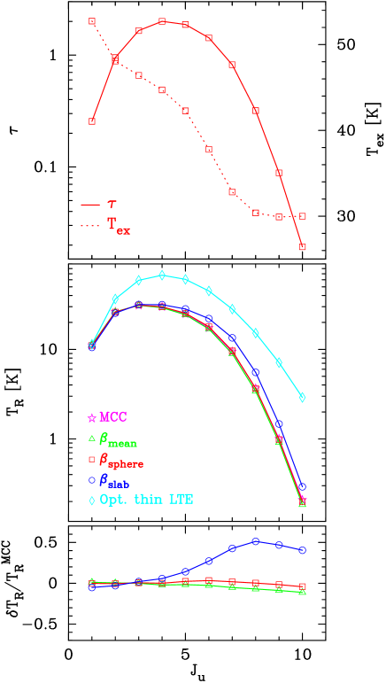
Figure 2: Comparison of the predicted line strengths for the 10 lowest rotational transitions of CO for a homogeneous isothermal sphere, with $n_{\mathrm{H_{2}}}=10^{5}$ cm^-3 and $T_{\mathrm{kin}}=50$ K, using different methods. Upper panel: The total optical depth through the sphere at line centre $\tau$ and excitation temperature $T_{\mathrm{ex}}$ as a function of the upper rotational level $J$ involved in the transition. Middle panel: The radiation temperature $T_{\mathrm{R}}$ obtained for each transition using RADEX with different prescriptions of the escape probability $\beta$ and compared with the result from the Monte-Carlo code (MCC) of Schöier (2000). Also shown are the results for optically thin emission in LTE. Lower panel: $T_{\mathrm{R}}$ obtained from RADEX compared with the results from MCC, $\delta T_{\mathrm{R}}=T_{\mathrm{R}}^{\mathrm{MCC}}-T_{\mathrm{R}}$.

3.5 Results

There are several ways in which RADEX can be used to analyze molecular line observations. In most of these applications, the modeled quantity is the velocity-integrated line intensity, as the excitation is assumed to be independent of velocity. As a consequence, self-absorbed lines cannot be modeled satisfactorily with RADEX. In the simplest case, the temperature and density are known from other observations and only the column density of the molecule under consideration needs to be varied to get the best agreement with the observed line intensity. If the H₂ column density is known from other observations, for example from an optically thin CO isotopic line, the ratio of the two column densities gives the molecular abundance, averaged over the source. The RADEX distribution contains a Python script to automate this procedure which is further described in Appendix D.

Another often-used application of RADEX is to determine temperatures and densities from the observed intensity ratios of lines of the same molecule. If the abundance of the molecule is constant throughout the source, the ratios should give source-averaged physical conditions independent of the specific chemistry of the molecule. Appendix C presents illustrative plots of line ratios for commonly observed molecules and lines in the optically thin case. For higher optical depths, the qualitative trends remain the same but there are quantitative differences. RADEX can readily be used to generate similar plots for moderately thick cases. Again, Python scripts are made available to automate this procedure (Appendix D).

To illustrate the use of RADEX on actual observations, we take the observations of the HCO⁺ 1–0 and 3–2 lines toward a relatively simple source, the photon-dominated region IC 63 (Jansen et al., 1994). The observed 1–0/3–2 ratio corrected for beam dilution is 5.5$\pm$1.5. The kinetic temperature of the source is constrained from CO observations to be $\sim$50 K. Fig. 9 shows that the inferred density for this ratio is then $\sim 5\times 10^{4}$ cm^-3, a value confirmed by other line ratios, e.g., CS 2–1/3–2. The inferred column density from the absolute intensities is $8\times 10^{12}$ cm^-2, which, together with the overall H₂ column density of $5\times 10^{21}$ cm^-2, gives an HCO⁺ abundance with respect to H₂ of $1.6\times 10^{-9}$.

A slightly more complicated situation arises for the Orion Bar PDR (Hogerheijde et al., 1995). For this source, both HCO⁺ 1–0, 3–2 and 4–3 lines have been observed. The 1–0/3–2 ratio gives an order of magnitude lower density than the 3–2/4–3 ratio. This difference in density automatically translates into an order of magnitude uncertainty in the inferred HCO⁺ column density, and thus the HCO⁺ abundance, since column density tracers such as CO are usually much less sensitive to density. One possible solution is a clumpy PDR model in which the 1–0 line is mostly produced in the low-density interclump gas containing 90% of the material and the 4–3 line in the high-density clumps. Within this clumpy model, a single column density fits all three lines and an accurate abundance can be derived. Note that this technique of adding the results of two models is only applicable at low optical depths.

If only two lines of a molecule have been observed, the line ratio can be used as indicator of temperature or density, depending on molecule and transition (Appendix C). A single line ratio is never enough to constrain both temperature and density, though. For multi-line observations, a comparison of data and models in terms of $\chi^{2}$ is preferred. See for example Van der Tak et al. (2000b), Schöier et al. (2002), and Leurini et al. (2004) for details of such calculations.

Figure 3: Excitation temperature of the HCO⁺ 1–0 transition as a function of radius for the model cloud of § 4.1.2, calculated with RADEX assuming static spherical, expanding spherical, and slab geometry (dashed / dash-dotted / dotted lines), with a multi-zone escape probability program (long/short dashes) and with a Monte Carlo code (solid lines). The panels are for different column densities, hence optical depths. Note the different vertical scales.

3.6 Limitations of the program

The current version of the program does not include a contribution from continuous (dust or free-free) opacity to the escape probability, as for example in Takahashi et al. (1983). Continuum radiation from dust is generally negligible at long wavelengths (${{}_{>}\atop{{}^{\sim}}}$1 mm) but becomes important for regions with very high column densities (such as protoplanetary disks) and at far-infrared and shorter wavelengths (${{}_{<}\atop{{}^{\sim}}}$100 $\mu$m). Free-free radiation may become important for the calculation of atomic fine structure lines from H II regions; other programs such as CLOUDY (Ferland, 2003) may be more suitable for this purpose. The absence of continuous opacity limits the applicability of the program particularly in situations where infrared pumping is important, either directly through rotational transitions or via vibrational transitions (Carroll & Goldsmith, 1981; Hauschildt et al., 1993).

Another limitation of the program is that only one molecule is treated at a time, so that the effects of line overlap are not taken into account. Such overlaps may occur both at radio and at infrared wavelengths (e.g., Expósito et al. 2006). In special cases, overlap between lines of the same molecule may influence their excitation, for example the hyperfine components of HCN or N₂H⁺ (Daniel et al., 2006).

For certain molecules under certain physical conditions (especially low density and/or strong radiation field), population inversions occur, which cause negative optical depth and hence nonlinear amplification of the incoming radiation (Elitzur, 1992). This phenomenon, known as ‘maser’ action, requires non-local treatment of the radiative transfer, in particular a fine sampling of directions, for which RADEX is not set up. Generally, the escape probability approximation is justified until the masers saturate, which occurs at $\tau\approx-1$. In practice, the computed intensities of lines with $\tau{{}_{<}\atop{{}^{\sim}}}-0.1$ are not as accurate as those of other lines, and the intensities of lines with $\tau{{}_{<}\atop{{}^{\sim}}}-1$ should be disregarded altogether. If many lines have negative optical depths, the intensities of non-maser lines may also be affected. While specialized programs should be used to calculate the intensities of maser lines (e.g., Spaans & van Langevelde, 1992; Gray & Field, 1995; Yates et al., 1997), RADEX may well be used to predict which lines of a molecule may display maser action under certain physical conditions. Note however that lines may be masers even if $\tau>0$ according to RADEX, for example ‘Class II’ CH₃OH masers which are pumped by infrared radiation (Leurini et al., 2004).

4 Comparison with other methods

This section shows a comparison of RADEX with other programs, first for the case of constant physical conditions (§ 4.1) and second for variable conditions (§ 4.2). Comparison is with the analytical rotation diagram method and with Monte Carlo methods, which have been benchmarked to high accuracy, both for the case of HCO⁺ (Van Zadelhoff et al., 2002) and of H₂O (Van der Tak et al., 2005). Throughout this section, molecular data have been taken from the LAMDA database (Schöier et al., 2005).

4.1 Homogeneous models

4.1.1 The case of CO

To test the RADEX code, we have compared its output both to an optically thin LTE analysis (rotation diagram method) and a full radiative transfer analysis using a Monte-Carlo method (Schöier, 2000). The test problem consists of a spherically symmetric cloud with a constant density, $n$(H₂), of $1\times 10^{5}$ cm^-3 within a radius of 100 AU. In this example only the CO emission is treated using a fractional abundance of $1\times 10^{-4}$ relative to H₂ yielding a central CO column density of $N_{\mathrm{CO}}=3\times 10^{16}$ cm^-2 and an average value of $N$=2$\times$10¹⁶ cm^-2. The kinetic temperature is set to 50 K, the background temperature to 2.73 K, and the line width to $\Delta$V=1.0 km s^-1.

Fig. 2 presents the results of the calculations for the ten lowest rotational transitions. The excitation temperatures of the lines vary from being close to thermalized for transitions involving low $J$-levels, to sub-thermally excited for the higher-lying lines. The optical depth in the lines is moderate ($\sim 1-2$) to low. It is seen that the expressions of the escape probability for the uniform sphere and the expanding sphere give almost identical solutions which are close to that obtained from the full radiative transfer (MCC in Fig. 2). The slab geometry gives slightly higher intensities, in particular for high-lying lines. The optically thin approximation, where the gas is assumed to be in LTE at 50 K, produces much larger discrepancies, up to a factor of $\sim 2$, and only gives the correct intensity for the $J=1\rightarrow 0$ line, where the LTE conditions are met.

4.1.2 The case of HCO⁺

To further verify the performance of the RADEX program, we have compared its results to that of another program that does not use the local approximation: the Monte Carlo program RATRAN (Hogerheijde & van der Tak, 2000). We also compare the results to those from the multi-zone escape probability program by Poelman & Spaans (2005). The test case is a cloud with $n$(H₂) = 1$\times$10⁴ cm^-3, $T_{\rm kin}$=10 K, $T_{\rm bg}$=2.73 K, and a line width of $\Delta$V=1.0 km s^-1, equivalent to $b_{D}$=0.6 km s^-1. The pure rotational emission spectrum of HCO⁺ was calculated for column densities of $10^{12}$, $10^{13}$, $10^{14}$ and $10^{15}$ cm^-2, which for RADEX were given directly as input parameters. For the multi-zone programs, a cloud radius of $10^{18}$ cm was specified along with abundances of $10^{-10}$–$10^{-7}$, distributed over 50 cells.

Figure 3 shows the calculated excitation temperature of the HCO⁺ 1–0 transition as a function of radius for these physical conditions. For $N$(HCO⁺)${{}_{<}\atop{{}^{\sim}}}$10¹² cm^-2, the excitation is independent of radius and the calculations for the various geometries agree to $\approx$10%. The dependence of the excitation on radius and on geometry increases with increasing column density, and for $N$(HCO⁺)${{}_{>}\atop{{}^{\sim}}}$10¹⁵ cm^-2, the curvature of the $T_{\rm ex}$ distribution becomes too large to ignore. The corresponding line optical depth is $\approx$100, with $\approx$20% spread between the various estimates (Fig. 4). The curvature arises because at the cloud center, photon trapping thermalizes the excitation, while at the edge, the emission can escape the cloud (Bernes, 1979). We do not recommend to use RADEX at line optical depths ${{}_{>}\atop{{}^{\sim}}}$100, because the calculated excitation temperature may not be representative of the emitting region. However, even if some lines are highly optically thick, RADEX may well be used to analyze other lines which are optically thin. For example for H₂O, the ground state lines often have $\tau\sim 1000$, but RADEX is well capable of computing intensities for higher-lying transitions which are not as optically thick.

At low optical depth, variations in $T_{\rm ex}$ translate directly into changes in emergent line intensity. Thus, differences as large as 20% in calculated line flux can arise depending on the choice of escape probability description, even for moderately thick cases. At high optical depth, the direct connection between $T_{\rm ex}$ and line flux is lost because of the dependence on the adopted velocity field. The assumption in the program that the optical depth is independent of velocity breaks down in this case. In this limit, the peak line temperature $T_{R}$ gives the value of $T_{\rm ex}$ at the $\tau=1$ surface of the cloud in this specific transition.

The results shown in this section do not translate easily to other HCO⁺ lines such as $J$=3$\to$2, because the excitation is governed by several competing effects. The optical depth of the $J$=3$\to$2 line may be higher or lower than that of the $J$=1$\to$0 line, depending on temperature and density. Observers are encouraged to use RADEX to study the excitation of their lines as a function of these parameters, and also consider geometric variations.

Figure 4: Optical depth of the HCO⁺ 1–0 transition for the model of § 4.1.2, calculated with RADEX assuming static spherical, expanding spherical, and slab geometry (filled triangles/filled squares/open triangles), with the multi-zone escape probability code (open circles) and with the Monte Carlo code (filled circles).

4.2 Observations of a Young Stellar Object

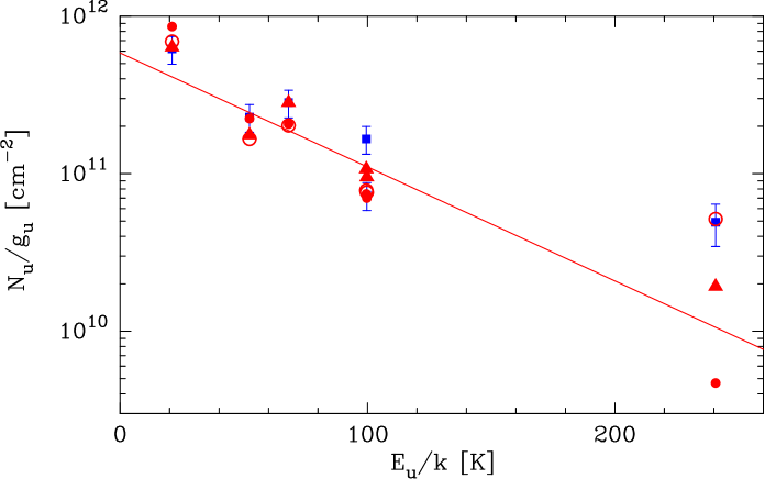
Figure 5: Line strengths of p-H₂CO observed towards the embedded low-mass protostar IRAS 16293–2422 (squares with error bars), modeled assuming LTE (solid line), using RADEX (triangles), and using a Monte Carlo program assuming a constant abundance (solid circles) and an abundance varying with radius (open circles).

Figure 6: Distributions of the $\chi^{2}$ parameter corresponding to the models in Figure 5. The RADEX results are for $n$(H₂) = 10⁶ cm^-3 as found by Van Dishoeck et al. (1995).

To compare a typical RADEX analysis with other methods for a situation which varying physical conditions, we choose a molecule for which many lines can be observed: para-formaldehyde, p-H₂CO. Figure 5 shows observations of p-H₂CO (sub-)millimeter emission lines originating from a wide range of energy levels toward the low-mass protostar IRAS 16293–2422 by Van Dishoeck et al. (1995). The data are analyzed using three methods: assuming LTE (with a rotation diagram), assuming SE (using RADEX), and using a Monte Carlo program. The free parameters for the LTE fit are the excitation temperature $T_{\rm ex}$ and the column density $N$(p-H₂CO). For the non-LTE fit, the free parameters are kinetic temperature $T_{\rm kin}$, H₂ density $n$(H₂), and $N$(p-H₂CO).

Figure 6 shows the distributions of the $\chi^{2}$ parameter for the LTE and SE fits, calculated in the standard way (see, e.g., Van der Tak et al. 2000b; Schöier et al. 2002) assuming a 20% uncertainty for all observed points except the line with the highest upper level energy where a 30% uncertainty was used. As seen from the figure, the non-LTE method gives a better fit to the data, as quantified by the lower minimum $\chi^{2}$ value. This result is not necessarily surprising given that more free parameters are available. A more important difference is that the estimates of temperature and column density between the two methods are substantially different, in particular the temperature (50 vs 150 K). Since the non-LTE method involves fewer assumptions about the physical state of the cloud, its results are to be preferred.

These results illustrate that rotation diagrams may give misleading results when determining physical properties of interstellar gas clouds (cf. Johnstone et al. 2003 for the case of CH₃OH). Figure 5 also demonstrates that temperatures and column densities derived from rotation diagrams tend to depend on which lines happen to have been observed (cf. the HCO⁺ case in § 4.1.2). From other data, IRAS 16293–2422 is actually known to have a gradient in temperature and density throughout its envelope, which cannot be modelled properly with either technique. For such situation, a full Monte Carlo radiative transfer method is needed in which both the physical conditions and the abundances can vary with radius (Fig. 5, circles). Nevertheless, the column densities and abundances inferred with RADEX using the physical conditions inferred from the line ratios differ by only a factor of a few from those found with the more sophisticated analysis, at least for the particular zone of the source to which those conditions apply (Schöier et al., 2002).

5 Conclusions

We have presented a computer program to analyze spectral line observations at radio and infrared wavelengths, based on the escape probability approximation. The program can be used for any molecule for which collisional data exist; such input data are available in the required format from the LAMDA database. The program can be used for optical depths from $\approx$–0.1 to $\approx$100.

The limited number of free parameters makes RADEX very useful to rapidly analyze large datasets. As an example, observed line intensity ratios may be compared with the plots in Appendix C to estimate density and kinetic temperature. Ratios of other lines and other molecules may be easily computed using the Python scripts included in the RADEX distribution. The program may also be used to create synthetic spectra. This capability will be important to model the THz line surveys from the HIFI instrument onboard the Herschel space observatory.

In the future, we plan to incorporate a multi-zone escape probability formalism (Poelman & Spaans, 2005; Elitzur & Asensio Ramos, 2006) which will enable models with varying physical conditions and also improve the performance of the program at high optical depths. To speed up convergence at high optical depths, the calculation may also start from LTE conditions rather than from optically thin statistical equilibrium. Robust convergence may be achieved by starting from either initial condition and requiring the two answers to be equal. For the modeling of crowded spectra, the effects of line overlap will also need to be considered, for instance in the ‘all or nothing’ approach (Cesaroni & Walmsley, 1991). Such spectra will be routinely observed with the superb resolution and sensitivity of ALMA.

Our program is free for anybody to use for science, provided that appropriate reference is made to this paper. For any other purpose such as to incorporate the program into other packages which may be distributed to the public, prior agreement with the authors is needed.

Appendix A Program input and output

A.1 Program input

The input parameters to RADEX are the following:

1. The name of the molecular data file to be used.

2. The name of the file to write the output to.

3. The frequency range for the output file [GHz]. All transitions from the molecular data file are always taken into account in the calculation, but often it is practical to write only a limited set of lines to the output.

4. The kinetic temperature of the cloud [K].

5. The number of collision partners to be used. Most users will want H₂ as only collision partner, but in more specialized cases, additional collisions with H or electrons may for instance play a role. See the molecular datafiles for details. For some species (CO, atoms) separate collision data for ortho and para H₂ exist; the program then uses the thermal ortho/para ratio unless the user specifies otherwise.

6. The name (case-insensitive) and the density [cm^-3] of each collision partner. Possibilities are H₂, p-H₂, o-H₂, electrons, atomic H, He, and H⁺.

7. The temperature of the background radiation field [K].

   • If $>$0, a black body at this temperature is used. Most users will adopt the cosmic microwave background at $T_{\rm CMB}$=2.725(1+$z$) K for a galaxy at redshift $z$.

   • If =0, the average interstellar radiation field (ISRF) is used, taken from Black (1994) with modifications described in § 3.2. This spectrum is not adjustable by a scale factor because it consists of several components that are not expected to scale linearly with respect to each other.

   • If $<$0, a user-defined radiation field is used, specified by values of frequency [cm^-1], intensity [Jy nsr^-1], and dilution factor [dimensionless]. Spline interpolation and extrapolation are applied to this table. The intensity need not be specified at all frequencies of the line list, but a warning message will appear if extrapolation (rather than interpolation) is required.

8. The column density of the molecule [cm^-2].

9. The FWHM line width [km s^-1].

A.2 Program output

The output file written by RADEX first replicates the input parameters, and then lists the following quantities for each spectral line within the specified frequency range.

1. Quantum numbers, upper state energy [K], frequency [GHz], and wavelength [$\mu$m]. These numbers are just copied from the molecular data file, which usually comes from the LAMDA database. Frequencies from this database are generally of spectroscopic accuracy (${{}_{<}\atop{{}^{\sim}}}$0.1 MHz uncertainty), although for the most precise values to be used for observations, the original literature and current line catalogs such as CDMS (Müller et al. 2001) should be consulted.

2. The excitation temperature [K] as defined in Eq. (10). In general, different lines have different excitation temperatures. Lines are thermalized if $T_{\rm ex}$=$T_{\rm kin}$; in LTE, all lines are thermalized.

3. The line optical depth, defined as the optical depth of the equivalent rectangular line shape ($\phi_{\nu}=1/\Delta\nu$).

4. The line intensity, defined as the Rayleigh-Jeans equivalent temperature $T_{R}$ [K].

5. The line flux, defined as the velocity-integrated intensity, both in units of K km s^-1 (common in radio astronomy) and of erg cm^-2 s^-1 (common in infrared astronomy). The line flux is calculated as 1.0645$T_{R}$$\Delta$V, where the factor 1.0645 = $\sqrt{\pi}/(2\sqrt{\ln 2})$ converts the adopted rectangular line profile into a Gaussian profile with an FWHM of $\Delta$V. The integrated profile is useful to estimate the total emission in the line, but it has limited meaning at high optical depths, because the change of optical depth over the line profile is not taken into account. Proper modeling of optically thick lines requires programs that resolve the source both spectrally and spatially (see § 4.1.2 for further discussion).

Auxiliary output files can be generated, for example to display the adopted continuum spectrum.

Appendix B Coding standards

The original version of RADEX was written in such a way as to minimize the use of machine memory which was expensive until a decade ago. Nowadays, clarity and easy maintenance are more important requirements, which is why the source code has been re-written following the rules below. We hope that these rules will be useful for the development of other ‘open source’ astronomical software. For further guidelines on scientific programming we recommend the Software Carpentry on-line course.

1. All the action is in subroutines; the sole purpose of the main program is to show the structure of the program. The subroutines are grouped into several files for a better overview; compilation instructions for automated builds on a variety of platforms are in a Makefile.

2. The program text is interspersed with comments at a ratio of $\approx$1:1. In particular, each subroutine starts with a description of its contents, its input and output, where incoming calls come from, and which calls go out. Then the properties of each variable are described: contents, units and type.

3. Variables and subroutines have descriptive names with a length of 5–10 letters. Names of integer variables start with the letters i..n; names of floating-point variables (always of double precision) with a..h or o..z. There are no specific namings for variables of character or logical type, as for example in CLOUDY. Names are always based on the English language. We do not use upper-, lower-, or camel-case to distinguish types of identifiers, as some programs do.

4. Loops are marked by indenting the program text. The loop variables are always called ilev, iline .., never just i.

5. Subroutines start with a check whether the input parameters have reasonable values. Such checks force soft landings if necessary, and avoid runtime errors.

6. Statements with calculations use spaces around the =, + and – symbols, but not around others. Calculations that consist of multiple steps are split over as many program lines. Multiple assignments in a row are aligned at the = sign.

7. The program text avoids “magic numbers” both in calculations and in definitions. Numbers that are often used such as Planck’s constant are defined at one central place in the program. Similarly, often-used variables such as physical parameters are stored in shared memory rather than passed on via subroutine calls.

Appendix C Diagnostic plots of molecular line ratios

We have used the RADEX program and the LAMDA database to calculate line ratios of several commonly observed molecules for a range of kinetic temperatures and H₂ densities. The plots in this Appendix may be used by observers to estimate physical conditions from their data. Line ratios have the advantage of being less sensitive to calibration errors than absolute line strengths, especially when the two lines have been measured with the same telescope, receiver and spectrometer.

The calculations assume a column density of 10¹² cm^-2, a line width of 1.0 km s^-1, and use a 2.73 K blackbody as background radiation field. Under these conditions, the lines are optically thin, so that the line ratios do not depend on column density. The calculations also assume that the emission in both lines fills the telescope beams equally, which may be the case if the lines are close in frequency. However, lines are generally measured in beams of different sizes, and the observations need to be corrected to account for this effect, if the source is known to be compact.

Linear molecules such as CO (Fig. 7) are tracers of density at low densities, when collisions compete with radiative decay. At higher densities, the excitation becomes thermalized and the line ratios are sensitive to temperature. For a given molecule, moving up the $J-$ladder means probing higher temperatures and densities. Note that for the column densities of typical dense interstellar clouds, the CO lines are optically thick, and observations of ¹³CO or even rarer isotopologues must be used to probe physical conditions.

The critical densities of molecular lines scale as $\mu^{2}\nu^{3}$, where $\mu$ is the permanent dipole moment of the molecule and $\nu$ is the frequency of the line. Indeed, the CS molecule (Fig. 8) has a larger dipole moment than CO, and its line ratios are mainly probes of the density. The small frequency spacing between the lines of CS makes this molecule very useful to probe density structure (e.g., Van der Tak et al. 2000b). The HCO⁺ and HCN molecules (Fig. 9) display similar trends to CS, although their line spacing is not as small.

Non-linear molecules such as H₂CO (Figs. 10 and 11) have the advantage that both temperature and density may be probed within the same frequency range. Ratios of lines from different $J-$states tend to be density tracers (left panels), while ratios of lines from the same $J-$state but different $K-$states are mostly temperature probes (right panels). The lines of H₂CO are often quite strong, making this molecule a favourite tracer of temperature and density (Mangum & Wootten 1993). Other asymmetric molecules have also been used, such as H₂CS (Blake et al. 1994) and CH₃OH (Leurini et al. 2004) although abundance variations from source to source or even within sources often complicate the interpretation (Johnstone et al. 2003).

Figure 7: Line ratios of CO in the optically thin limit as a function of kinetic temperature and H₂ density. Contours are spaced linearly and some contours are labeled for easy identification.

Figure 8: Line ratios of CS in the optically thin limit as a function of kinetic temperature and H₂ density. Contours are spaced linearly and some contours are labeled for easy identification.

Figure 9: Line ratios of HCO⁺ and HCN in the optically thin limit as a function of kinetic temperature and H₂ density. Contours are spaced linearly and some contours are labeled for easy identification.

Figure 10: Line ratios of o-H₂CO in the optically thin limit as a function of kinetic temperature and H₂ density. Contours are spaced linearly and some contours are labeled for easy identification.

Figure 11: Line ratios of p-H₂CO in the optically thin limit as a function of kinetic temperature and H₂ density. Contours are spaced linearly and some contours are labeled for easy identification.

Appendix D The Python scripts

The RADEX distribution comes with two scripts, radex_line.py and radex_grid.py, to automate standard modeling procedures. The scripts are written in Python and are run from the Unix shell command line after manual editing of parameters.

The first script, radex_line.py, calculates the column density of a molecule from an observed line intensity, given estimates of kinetic temperature and H₂ volume density. The input parameters are:

1. The kinetic temperature [K]

2. The number density of H₂ molecules [cm^-3]

3. The temperature of the background radiation field [K], usually 2.73 (CMB).

4. The name of the molecule (or molecular data file)

5. The frequency of the line [GHz]

6. The observed line intensity [K]

7. The observed line width [km s^-1]

Furthermore, two numerical parameters have good default values but will need to be changed occasionally:

1. The free spectral range around the line (default 10%): this number must be smaller for molecules with many line close in frequency, such as CH₃OH. The program uses this parameter to find the observed line from the list of lines in the molecular model.

2. The required accuracy (default 10%): The default corresponds to the calibration uncertainty of most telescopes.

The script iterates on column density until the observed and modeled line fluxes agree to within the desired accuracy. The best-fit column density is directly written to the screen. The file radex.out gives details of the best-fit model.

The second script, radex_grid.py, runs a series of RADEX models to estimate the kinetic temperature and/or the volume density from an observed line ratio. The user needs to set the following input parameters:

1. The grid boundaries: minimum and maximum kinetic temperature [K] and minimum and maximum H₂ volume density [cm^-3].

2. The temperature of the background radiation field [K], usually 2.73 (CMB).

3. The molecular column density [cm^-2]. For the illustrative plots in Appendix C, a low value ($N$=10¹² cm^-2) was used, so that the line ratios are independent of column density (optically thin limit). However, in modeling specific observations, it is worth varying this parameter to assess the sensitivity of the line ratio to column density.

4. The observed line width [km s^-1], usually an average of the widths of the two lines.

The numerical parameters which have good default values but will need to be changed occasionally are:

1. The number of grid points along the temperature and density axes.

2. The free spectral range around the line (see above)

The name of the molecule and a list of observed line ratios and names of associated output files are given at the start of the main program. The script produces a file radex.out which is a tabular listing of temperature, log density, and line ratio. This results may be plotted with the user’s favourite plotting program.