Placeholder Substructures III:   A Bit-String-Driven “Recipe Theory” for Infinite-Dimensional Zero-Divisor Spaces

Abstract

Zero-divisors (ZDs) derived by Cayley-Dickson Process (CDP) from N-dimensional hypercomplex numbers ($N$ a power of $2$, and at least $4$) can represent singularities and, as $N\rightarrow\infty$, fractals – and thereby, scale-free networks. Any integer $>8$ and not a power of $2$ generates a meta-fractal or Sky when it is interpreted as the strut constant (S) of an ensemble of octahedral vertex figures called Box-Kites (the fundamental ZD building blocks). Remarkably simple bit-manipulation rules or recipes provide tools for transforming one fractal genus into others within the context of Wolfram’s Class 4 complexity.

1 The Argument So Far

In Parts I[1] and II[2], the basic facts concerning zero-divisors (ZDs) as they arise in the hypercomplex context were presented and proved. “Basic,” in the context of this monograph, means seven things. First, they emerged as a side-effect of applying CDP a minimum of 4 times to the Real Number Line, doubling dimension to the Complex Plane, Quaternion 4-Space, Octonion 8-Space, and 16-D Sedenions. With each such doubling, new properties were found: as the price of sacrificing counting order, the Imaginaries made a general theory of equations and solution-spaces possible; the non-commutative nature of Quaternions mapped onto the realities of the manner in which forces deploy in the real world, and led to vector calculus; the non-associative nature of Octonions, meanwhile, has only come into its own with the need for necessarily unobservable quantities (because of conformal field-theoretical constraints)in String Theory. In the Sedenions, however, the most basic assumptions of all – well-defined notions of field and algebraic norm (and, therefore, measurement) – break down, as the phenomena correlated with their absence, zero-divisors, appear onstage (never to leave it for all higher CDP dimension-doublings).

Second thing: ZDs require at least two differently-indexed imaginary units to be defined, the index being an integer larger than 0 (the CDP index of the Real Unit) and less than $2^{N}$ for a given CDP-generated collection of $2^{N}$-ions. In “pure CDP,” the enormous number of alternative labeling schemes possible in any given $2^{N}$-ion level are drastically reduced by assuming that units with such indices interact by XOR-ing: the index of the product of any two is the XOR of their indices. Signing is more tricky; but, when CDP is reduced to a 2-rule construction kit, it becomes easy: for index $u<{\bf G}$, ${\bf G}$ the Generator of the $2^{N}$-ions (i.e., the power of 2 immediately larger than the highest index of the predecessor $2^{N-1}$-ions), Rule 1 says $i_{u}\cdot i_{\bf G}=+i_{(u+{\bf G})}$. Rule 2 says take an associative triplet $(a,b,c)$, assumed written in CPO (short for “cyclically positive order”: to wit, $a\cdot b=+c$, $b\cdot c=+a$, and $c\cdot a=+b$). Consider, for instance, any $(u,{\bf G},{\bf G}+u)$ index set. Then three more such associative triplets (henceforth, trips) can be generated by adding G to two of the three, then switching their resultants’ places in the CPO scheme. Hence, starting with the Quaternions’ $(1,2,3)$ (which we’ll call a Rule 0 trip, as it’s inherited from a prior level of CDP induction), Rule 1 gives us the trips $(1,4,5)$, $(2,4,6)$, and $(3,4,7)$, while Rule 2 yields up the other 4 trips defining the Octonions: $(1,7,6)$, $(2,5,7)$, and $(3,6,5)$. Any ZD in a given level of $2^{N}$-ions will then have units with one index $<{\bf G}$, written in lowercase, and the other index $>{\bf G}$, written in uppercase. Such pairs, alternately called “dyads” or “Assessors,” saturate the diagonal lines of their planes, which diagonals never mutually zero-divide each other (or make DMZs, for ”divisors (or dyads) making zero”), but only make DMZs with other such diagonals, in other such Assessors. (This is, of course, the opposite situation from the projection operators of quantum mechanics, which are diagonals in the planes formed by Reals and dimensions spanned by Pauli spin operators contained within the 4-space created by the Cartesian product of two standard imaginaries.)

Third thing: Such ZDs are not the only possible in CDP spaces; but they define the “primitive” variety from which ZD spaces saturating more than 1-D regions can be articulated. A not quite complete catalog of these can be found in our first monograph on the theme [3]; a critical kind which was overlooked there, involving the Reals (and hence, providing the backdrop from which to see the projection-operator kind as a degenerate type), were first discussed more recently [4]. (Ironically, these latter are the easiest sorts of composites to derive of any: place the two diagonals of a DMZ pairing with differing internal signing on axes of the same plane, and consider the diagonals they make with each other!) All the primitive ZDs in the Sedenions can be collected on the vertices of one of 7 copies of an Octahedron in the Box-Kite representation, each of whose 12 edges indicates a two-way “DMZ pathway,” evenly divided between 2 varieties. For any vertex V, and $k$ any real scalar, indicate the diagonals this way: $\verb|(V,/)|=k\cdot(i_{v}+i_{V})$, while $\verb|(V, \)|=k\cdot(i_{v}-i_{V})$. 6 edges on a Box-Kite will always have negative edge-sign (with unmarked ET cell entries: see the “sixth thing”). For vertices M and N, exactly two DMZs run along the edge joining them, written thus:

$\verb|(M,/)|\cdot\verb|(N, \)|$ $=\verb|(M, \)|$ $\cdot$ $\verb|(N,/)|$ $=0$

The other 6 all have positive edge-sign, the diagonals of their two DMZs having same slope (and marked – with leading dashes – ET cell entries):

$\verb|(Z,/)|\cdot\verb|(V, /)|=$ $\verb|(Z, \)|\cdot\verb|(V,\)|=0$

Fourth thing: The edges always cluster similarly, with two opposite faces among the 8 triangles on the Box-Kite being spanned by 3 negative edges (conventionally painted red in color renderings), with all other edges being positive (painted blue). One of the red triangles has its vertices’ 3 low-index units forming a trip; writing their vertex labels conventionally as A, B, C, we find there are in fact always 4 such trips cycling among them: $(a,b,c)$, the L-trip; and the three U-trips obtained by replacing all but one of the lowercase labels in the L-trip with uppercase: $(a,B,C)$; $(A,b,C)$; $(A,B,c)$. Such a 4-trip structure is called a Sail, and a Box-Kite has 4 of them: the Zigzag, with all negative edges, and the 3 Trefoils, each containing two positive edges extending from one of the Zigzag vertices to the two vertices opposite its Sailing partners. These opposite vertices are always joined by one of the 3 negative edges comprising the Vent which is the Zigzag’s opposite face. Again by convention, the vertices opposite A, B, C are written F, E, D in that order; hence, the Trefoil Sails are written $(A,D,E)$; $(F,D,B)$, and $(F,C,E)$, ordered so that their lowercase renderings are equivalent to their CPO L-trips. The graphical convention is to show the Sails as filled in, while the other 4 faces, like the Vent, are left empty: they show “where the wind blows” that keeps the Box-Kite aloft. A real-world Box-Kite, meanwhile, would be held together by 3 dowels (of wood or plastic, say) spanning the joins between the only vertices left unconnected in our Octahedral rendering: the Struts linking the strut-opposite vertices (A, F); (B, E); (C, D).

Fifth thing: In the Sedenions, the 7 isomorphic Box-Kites are differentiated by which Octonion index is missing from the vertices, and this index is designated by the letter S, for “signature,” “suppressed index,” or strut constant. This last designation derives from the invariant relationship obtaining in a given Box-Kite between S and the indices in the Vent and Zigzag termini (V and Z respectively) of any of the 3 Struts, which we call the “First Vizier” or VZ1. This is one of 3 rules, involving the three Sedenion indices always missing from a Box-Kite’s vertices: ${\bf G}$, ${\bf S}$, and their simple sum ${\bf X}$ (which is also their XOR product, since ${\bf G}$ is always to the left of the left-most bit in ${\bf S}$). The Second Vizier tells us that the L-index of either terminus with the U-index of the other always form a trip with ${\bf G}$, and it true as written for all $2^{N}$-ions. The Third shows the relationship between the L- and U- indices of a given Assessor, which always form a trip with ${\bf X}$. Like the First, it is true as written only in the Sedenions, but as an unsigned statement about indices only, it is true universally. (For that reason, references to VZ1 and VZ3 hereinout will be assumed to refer to the unsigned versions.) First derived in the last section of Part I, reprised in the intro of Part II, we write them out now for the third and final time in this monograph:

VZ1: $v\cdot z=V\cdot Z={\bf S}$

VZ2: $Z\cdot v=V\cdot z={\bf G}$

VZ3: $V\cdot v=z\cdot Z={\bf X}$.

Rules 1 and 2, the Three Viziers, plus the standard Octonion labeling scheme derived from the simplest finite projective group, usually written as PSL(2,7), provide the basis of our toolkit. This last becomes powerful due to its capacity for recursive re-use at all levels of CDP generation, not just the Octonions. The simplest way to see this comes from placing the unique Rule 0 trip provided by the Quaternions on the circle joining the 3 sides’ midpoints, with the Octonion Generator’s index, 4, being placed in the center. Then the 3 lines leading from the Rule 0 trip’s (1, 2, 3) midpoints to their opposite angles – placed conventionally in clockwise order in the midpoints of the left, right, and bottom sides of a triangle whose apex is at 12 o’clock – are CPO trips forming the Struts, while the 3 sides themselves are the Rule 2 trips. These 3 form the L-index sets of the Trefoil Sails, while the Rule 0 trip provides the same service for the Zigzag. By a process analogized to tugging on a slipcover (Part I) and pushing things into the central zone of hot oil while wok-cooking (Part II), all 7 possible values of S in the Sedenions, not just the 4, can be moved into the center while keeping orientations along all 7 lines of the Triangle unchanged. Part II’s critical Roundabout Theorem tells us, moreover, that all $2^{N}$-ion ZDs, for all $N>3$, are contained in Box-Kites as their minimal ensemble size. Hence, by placing the appropriate ${\bf G}$, ${\bf S}$, or ${\bf X}$ in the center of a PSL(2,7) triangle, with a suitable Rule 0 trip’s indices populating the circle, any and all candidate primitive ZDs can be discovered and situated.

Sixth thing: The word “candidate” in the above is critical; its exploration was the focus of Part II. For, starting with $N=5$ and hence ${\bf G=16}$ (which is to say, in the 32-D Pathions), whole Box-Kites can be suppressed (meaning, all 12 edges, and not just the Struts, no longer serve as DMZ pathways). But for all $N$, the full set of candidate Box-Kites are viable when ${\bf S}\leq 8$ or equal to some higher power of 2. For all other ${\bf S}$ values, though, the phenomenon of carrybit overflow intervenes – leading, ultimately, to the “meta-fractal” behavior claimed in our abstract. To see this, we need another mode of representation, less tied to 3-D visualizing, than the Box-Kite can provide. The answer is a matrix-like method of tabulating the products of candidate ZDs with each other, called Emanation Tables or ETs. The L-indices only of all candidate ZDs are all we need indicate (the U-indices being forced once ${\bf G}$ is specified); these will saturate the list of allowed indices $<{\bf G}$, save for the value of ${\bf S}$ whose choice, along with that of ${\bf G}$, fixes an ET. Hence, the unique ET for given ${\bf G}$ and ${\bf S}$ will fill a square spreadsheet whose edge has length $2^{N-1}-2$. Moreover, a cell entry (r,c) is only filled when row and column labels R and C form a DMZ, which can never be the case along an ET’s long diagonals: for the diagonal starting in the upper left corner, R xor R = 0, and the two diagonals within the same Assessor, can never zero-divide each other; for the righthand diagonal, the convention for ordering the labels (ascending counting order from the left and top, with any such label’s strut-opposite index immediately being entered in the mirror-opposite positions on the right and bottom) makes R and C strut-opposites, hence also unable to form DMZs.

For the Sedenions, we get a 6 x 6 table, 12 of whose cells (those on long diagonals) are empty: the 24 filled cells, then, correspond to the two-way traffic of “edge-currents” one imagines flowing between vertices on a Box-Kite’s 12 edges. A computational corollary to the Roundabout Theorem, dubbed the Trip-Count Two-Step, is of seminal importance. It connects this most basic theorem of ETs to the most basic fact of associative triplets, indicated in the opening pages of Part I, namely: for any N, the number $Trip_{N}$ of associative triplets is found, by simple combinatorics, to be $(2^{N}-1)(2^{N}-2)/3!$ – 35 for the Sedenions, 155 for the Pathions, and so on. But, by Trip-Count Two-Step, we also know that the maximum number of Box-Kites that can fill a $2^{N}$-ion ET = $Trip_{N-2}$. For ${\bf S}$ a power of 2, beginning in the Pathions (for ${\bf S}=2^{5-2}=8$), the Number Hub Theorem says the upper left quadrant of the ET is an unsigned multiplication table of the $2^{N-2}$-ions in question, with the 0’s of the long diagonal (indicated Real negative units) replaced by blanks – a result effectively synonymous with the Trip-Count Two-Step.

Seventh thing: We found, as Part II’s argument wound down, that the 2 classes of ETs found in the Pathions – the “normal” for ${\bf S}\leq 8$, filled with indices for all 7 possible Box-Kites, and the “sparse” so-called Sand Mandalas, showing only 3 Box-Kites when $8<{\bf S}<16$, were just the beginning of the story. A simple formula involving just the bit-string of ${\bf s}$ and ${\bf g}$, where the lowercase indicates the values of ${\bf S}$ and ${\bf G}$ modulo ${\bf G}/2$, gave the prototype of our first recipe: all and only cells with labels R or C, or content P ( = R xor C ), are filled in the ET. The 4 “missing Box-Kites” were those whose L-index trip would have been that of a Sail in the $2^{N-1}$ realm with ${\bf S}={\bf s}$ and ${\bf G}={\bf g}$. The sequence of 7 ETs, viewed in ${\bf S}$-increasing succession, had an obvious visual logic leading to their being dubbed a flip-book. These 7 were obviously indistinguishable from many vantages, hence formed a spectrographic band. There were 3 distinct such bands, though, each typified by a Box-Kite count common to all band-members, demonstrable in the ETs for the 64-D Chingons. Each band contained ${\bf S}$ values bracketed by multiples of 8 (either less than or equal to the higher, depending upon whether the latter was or wasn’t a power of 2). These were claimed to underwrite behaviors in all higher $2^{N}$-ion ETs, according to 3 rough patterns in need of algorithmic refining in this Part III. Corresponding to the first unfilled band, with ETs always missing $4^{N-4}$ of their candidate Box-Kites for $N>4$, we spoke of recursivity, meaning the ETs for constant ${\bf S}$ and increasing $N$ would all obey the same recipe, properly abstracted from that just cited above, empirically found among the Pathions for ${\bf S}>8$. The second and third behaviors, dubbed, for ${\bf S}$ ascending, (s,g)-modularity and hide/fill involution respectively, make their first showings in the Chingons, in the bands where $16<{\bf S}\leq 24$, and then where $24<{\bf S}<32$. In all such cases, we are concerned with seeing the “period-doubling” inherent in CDP and Chaotic attractors both become manifest in a repeated doubling of ET edge-size, leading to the fixed-${\bf S}$, $N$ increasing analog of the fixed-$N,{\bf S}$ increasing flip-books first observed in the Pathions, which we call balloon-rides. Specifying and proving their workings, and combining all 3 of the above-designated behaviors into the “fundamental theorem of zero-division algebra,” will be our goals in this final Part III. Anyone who has read this far is encouraged to bring up the graphical complement to this monograph, the 78-slide Powerpoint show presented at NKS 2006 [5], in another window. (Slides will be referenced by number in what follows.)

2 $8<{\bf S}<16,N\rightarrow\infty$ : Recursive Balloon Rides in the Whorfian Sky

We know that any ET for the $2^{N}$-ions is a square whose edge is $2^{N-1}-2$ cells. How, then, can any simply recursive rule govern exporting the structure of one such box to analogous boxes for progressively higher $N$? The answer: include the label lines – not just the column and row headers running across the top and left margins, but their strut-opposite values, placed along the bottom and right margins, which are mirror-reversed copies of the label-lines (LLs) proper to which they are parallel. This increases the edge-size of the ET box to $2^{N-1}$.

Theorem 11. For any fixed ${\bf S}>8$ and not a power of $2$, the row and column indices comprising the Label Lines (LLs) run along the left and top borders of the $2^{N}$-ion ET ”spreadsheet” for that ${\bf S}$. Treat them as included in the spreadsheet, as labels, by adding a row and column to the given square of cells, of edge $2^{N-1}-2$, which comprises the ET proper. Then add another row and column to include the strut-opposite values of these labels’ indices in “mirror LLs,” running along the opposite edges of a now $2^{N-1}$-edge-length box, whose four corner cells, like the long diagonals they extend, are empty. When, for such a fixed ${\bf S}$, the ET for the $2^{N+1}$-ions is produced, the values of the 4 sets of LL indices, bounding the contained $2^{N}$-ion ET, correspond, as cell values, to actual DMZ P-values in the bigger ET, residing in the rows and columns labeled by the contained ET’s ${\bf G}$ and ${\bf X}$ (the containing ET’s $g$ and $g+{\bf S}$). Moreover, all cells contained in the box they bound in the containing ET have P-values (else blanks) exactly corresponding to – and including edge-sign markings of – the positionally identical cells in the $2^{N}$-ion ET: those, that is, for which the LLs act as labels.

Proof. For all strut constants of interest, ${\bf S}<g(={\bf G/2})$; hence, all labels up to and including that immediately adjoining its own strut constant (that is, the first half of them) will have indices monotonically increasing, up to and at least including the midline bound, from $1$ to $g-1$. When $N$ is incremented by $1$, the row and column midlines separating adjoining strut-opposites will be cut and pulled apart, making room for the labels for the $2^{N+1}$-ion ET for same ${\bf S}$, which middle range of label indices will also monotonically increase, this time from the current $2^{N}$-ion generation’s $g$ (and prior generation’s ${\bf G}$), up to and at least including its own midline bound, which will be $g$ plus the number of cells in the LL inherited from the prior generation, or $g/2-1$. The LLs are therefore contained in the rows and columns headed by $g$ and its strut opposite, $g+{\bf S}$. To say that the immediately prior CDP generation’s ET labels are converted to the current generation’s P-values in the just-specified rows and columns is equivalent to asserting the truth of the following calculation:

$(g+u)+(sg)\cdot({\bf G}+g+u_{opp})$

$\;\;\;\;\;\;g\;\;\;\;\;+\;\;\;\;\;({\bf G}+g+{\bf S})\;\;\;\;\;\;$

$-(vz)\cdot({\bf G}+u_{opp})\;\;\;+(vz)\cdot(sg)\cdot u$

$+u\;\;\;\;\;-\;\;\;\;\;(sg)\cdot({\bf G}+u_{opp})$

$0$ only if $vz=(-sg)$

Here, we use two binary variables, the inner-sign-setting $sg$, and the Vent-or-Zigzag test, based on the First Vizier. Using the two in tandem lets us handle the normal and “Type II” box-kites in the same proof. Recall (and see Appendix B of Part II for a quick refresher) that while the “Type I” is the only type we find in the Sedenions, we find that a second variety emerges in the Pathions, indistinguishable from Type I in most contexts of interest to us here: the orientation of 2 of the 3 struts will be reversed (which is why VZ1 and VZ3 are only true generally when unsigned). For a Type I, since ${\bf S}<g$, we know by Rule 1 that we have the trip $({\bf S},g,g+{\bf S})$; hence, $g$ – for all $2^{N}$-ions beyond the Pathions, where the Sand Mandalas’ $g=8$ is the L-index of the Zigzag B Assessor – must be a Vent (and its strut-opposite, $g+{\bf S}$, a Zigzag). For a Type II, however, this is necessarily so only for 1 of the 3 struts – which means, per the equation above, that sg must be reversed to obtain the same result. Said another way, we are free to assume either signing of $vz$ means +1, so the “only if” qualifying the zero result is informative. It is $u$ and its relationship to $g+u$ that is of interest here, and this formulation makes it easier to see that the products hold for arbitrary LL indices $u$ or their strut-opposites. But for this, the term-by-term computations should seem routine: the left bottom is the Rule 1 outcome of $(u,g,g+u)$: obviously, any $u$ index must be less than $g$. To its right, we use the trip $(u_{opp},g,g+u_{opp})\rightarrow({\bf G}+g+u_{opp},g,{\bf G}+u_{opp})$, whose CPO order is opposite that of the multiplication. For the top left, we use $(u,{\bf S},u_{opp})$ as limned above, then augment by $g$, then ${\bf G}$, leaving $u_{opp}$ unaffected in the first augmenting, and $g+u$ in the second. Finally, the top right (ignoring $sg$ and $vz$ momentarily) is obtained this way: $(u,{\bf S},u_{opp})\rightarrow(u,g+u_{opp},g+{\bf S})\rightarrow(u,{\bf G}+g+s,{\bf G}+g+u_{opp})$; ergo, $+u$.

Note that we cannot eke out any information about edge-sign marks from this setup: since labels, as such, have no marks, we have nothing to go on – unlike all other cells which our recursive operations will work on. Indeed, the exact algorithmic determination of edge-sign marks for labels is not so trivial: as one iterates through higher $N$ values, some segments of LL indexing will display reversals of marks found in the ascending or descending left midline column, while other segments will show them unchanged – with key values at the beginnings and ends of such octaves (multiples of $8$, and sums of such multiples with ${\bf S}\;mod\;8$) sometimes being reversed or kept the same irrespective of the behavior of the terms they bound. Fortunately, such behaviors are of no real concern here – but they are, nevertheless, worth pointing out, given the easy predictability of other edge-sign marks in our recursion operations.

Now for the ET box within the labels: if all values (including edge-sign marks) remain unchanged as we move from the $2^{N}$-ion ET to that for the $2^{N+1}$-ions, then one of 3 situations must obtain: the inner-box cells have labels $u,v$ which belong to some Zigzag L-trip $(u,v,w)$; or, on the contrary, they correspond to Vent L-indices – the first two terms in the CPO triplet $(w_{opp},v_{opp},u)$, for instance; else, finally, one term is a Vent, the other a Zigzag (so that inner-signs of their multiplied dyads are both positive): we will write them, in CPO order, $v_{opp}$ and $u$, with third trip member $w_{opp}$. Clearly, we want all the products in the containing ET to indicate DMZs only if the inner ET’s cells do similarly. This is easily arranged: for the containing ET’s cells have indices identical to those of the contained ET’s, save for the appending of $g$ to both (and ditto for the U-indices).

Case 1: If $(u,v,w)$ form a Zigzag L-index set, then so do $(g+v,g+u,w)$, so markings remain unchanged; and if the $(u,v)$ cell entry is blank in the contained, so will be that for $(g+u,g+v)$ in its container. In other words, the following holds:

$(g+v)+(sg)\cdot({\bf G}+g+v_{opp})$

$\;\;\;(g+u)\;\;\;\;+\;\;\;({\bf G}+g+u_{opp})\;\;\;$

$-({\bf G}+w_{opp})\;\;\;-(sg)\cdot w$

$-w\;\;\;\;\;-(sg)\cdot({\bf G}+w_{opp})$

$0$ only if $sg=(-1)$

$(g+u)\cdot(g+v)=P:$ $(u,v,w)\rightarrow(g+v,g+u,w)$; hence, $(-w)$.

$(g+u)\cdot(sg)\cdot({\bf G}+g+v_{opp})=P:$ $(u,w_{opp},v_{opp})$ $\rightarrow(g+v_{opp},w_{opp},g+u)$ $\rightarrow({\bf G}+w_{opp},{\bf G}+g+v_{opp},g+u)$; hence, $(sg)\cdot(-({\bf G}+w_{opp}))$.

$({\bf G}+g+u_{opp})\cdot(g+v)=P:$ $(u_{opp},w_{opp},v)$ $\rightarrow(g+v,w_{opp},g+u_{opp})$ $\rightarrow(g+v,{\bf G}+g+u_{opp},{\bf G}+w_{opp})$; hence, $(-({\bf G}+w_{opp}))$.

$({\bf G}+g+u_{opp})\cdot({\bf G}+g+v_{opp})=P:$ Rule 2 twice to the same two terms yields the same result as the terms in the raw, hence $(-w)$.

Clearly, cycling through $(u,v,w)$ to consider $(g+v)\cdot(g+w)$ will give the exactly analogous result, forcing two (hence three) negative inner-signs in the candidate Sail; hence, if we have DMZs at all, we have a Zigzag Sail.

Case 2: The product of two Vents must have negative edge-sign, and there’s no cycling through same-inner-signed products as with the Zigzag, so we’ll just write our setup as a one-off, with upper inner-sign explicitly negative, and claim its outcome true.

$(g+v_{opp})-({\bf G}+g+v)$

$\;(g+w_{opp})\;+\;({\bf G}+g+w)\;$

$+({\bf G}+u_{opp})\;\;\;\;\;+u$

$-u\;\;\;\;\;-({\bf G}+u_{opp})$

$0$

$(g+w_{opp})\cdot(g+v_{opp})=P:$ $(w_{opp},v_{opp},u)$ $\rightarrow(g+v_{opp},g+w_{opp},u)$; hence, $(-u)$.

$(g+w_{opp})\cdot({\bf G}+g+v)=P:$ $(w_{opp},v,u_{opp})$ $\rightarrow(g+v,g+w_{opp},u_{opp})$ $\rightarrow({\bf G}+u_{opp},g+w_{opp},{\bf G}+g+v)$; but inner sign of upper dyad is negative, so $(-({\bf G}+u_{opp}))$.

$({\bf G}+g+w)\cdot(g+v_{opp})=P:$ $(v_{opp},u_{opp},w)$ $\rightarrow(g+w,u_{opp},g+v_{opp})$ $\rightarrow({\bf G}+u_{opp},{\bf G}+g+w,g+v_{opp})$; hence, $(+({\bf G}+u_{opp}))$.

$({\bf G}+g+w)\cdot({\bf G}+g+v)=P:$ Rule 2 twice to the same two terms yields the same result as the terms in the raw; but inner sign of upper dyad is negative, so $(+u)$.

Case 3: The product of Vent and Zigzag displays same inner sign in both dyads; hence the following arithmetic holds:

$(g+u)+({\bf G}+g+u_{opp})$

$\;(g+v_{opp})\;+\;({\bf G}+g+v)\;$

$-({\bf G}+w)\;\;\;\;\;+w_{opp}$

$-w_{opp}\;\;\;\;\;+({\bf G}+w)$

$0$

The calculations are sufficiently similar to the two prior cases as to make their writing out tedious. It is clear that, in each of our three cases, content and marking of each cell in the contained ET and the overlapping portion of the container ET are identical. $\;\;\blacksquare$

To highlight the rather magical label/content involution that occurs when $N$ is in- or de- cremented, graphical realizations of such nested patterns, as in Slides 60-61, paint LLs (and labels proper) a sky-blue color. The bottom-most ET being overlaid in the central box has $g=$ the maximum high-bit in ${\bf S}$, and is dubbed the inner skybox. The degree of nesting is strictly measured by counting the number of bits $B$ that a given skybox’s $g$ is to the left of this strut-constant high-bit. If we partition the inner skybox into quadrants defined by the midlines, and count the number $Q$ of quadrant-sized boxes along one or the other long diagonal, it is obvious that the inner skybox itself has $B=0$ and $Q=1$; the nested skyboxes containing it have $Q=2^{B}$. If recursion of skybox nesting be continued indefinitely – to the fractal limit, which terminology we will clarify shortly – the indices contained in filled cells of any skybox can be interpreted in $B$ distinct ways, $B\rightarrow\infty$, as representations of distinct ZDs with differing ${\bf G}$ and, therefore, differing U-indices. By obvious analogy to the theory of Riemann surfaces in complex analysis, each such skybox is a separate “sheet”; as with even such simple functions as the logarithmic, the number of such sheets is infinite. We could then think of the infinite sequence of skyboxes as so many cross-sections, at constant distances, of a flashlight beam whose intensity (one over the ET’s cell count) follows Kepler’s inverse square law. Alternatively, we could ignore the sheeting and see things another way.

Where we called fixed-$N$, ${\bf S}$ varying sequences of ETs flip-books, we refer to fixed-${\bf S}$, $N$ varying sequences as balloon rides: the image is suggested by David Niven’s role as Phineas Fogg in the movie made of Jules Vernes’ Around the World in 80 Days: to ascend higher, David would drop a sandbag over the side of his hot-air balloon’s basket; if coming down, he would pull a cord that released some of the balloon’s steam. Each such navigational tactic is easy to envision as a bit-shift, pushing ${\bf G}$ further to the left to cross LLs into a higher skybox, else moving it rightward to descend. Using ${\bf S=15}$ as the basis of a 3-stage balloon-ride, we see how increasing $N$ from $5$ to $6$ to $7$ approaches the white-space complement of one of the simplest (and least efficient) plane-filling fractals, the Cesàro double sweep [6, p. 65].

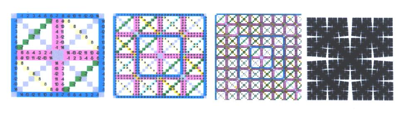
Figure 1: ETs for S=15, N=5,6,7 (nested skyboxes in blue)$\cdots$ and “fractal limit.”

The graphics were programmatically generated prior to the proving of the theorems we’re elaborating: their empirical evidence was what informed (indeed, demanded) the theoretical apparatus. And we are not quite finished with the current task the apparatus requires of us. We need two more theorems to finish the discussion of skybox recursion. For both, suppose some skybox with $B=k$, $k$ any non-negative integer, is nested in one with $B=k+1$. Divide the former along midlines to frame its four quadrants, then block out the latter skybox into a $4\times 4$ grid of same-sized window panes, partitioned by the one-cell-thick borders of its own midlines into quadrants, each of which is further subdivided by the outside edges of the 4 one-cell-thick label lines and their extensions to the window’s frame. These extended LLs are themselves NSLs, and have $R,C$ values of $g$ and $g+{\bf S}$; for ${\bf S}=15$, they also adjoin NSLs along their outer edges whose $R,C$ values are multiples of $8$ plus ${\bf S}\;mod\;8$. These pane-framing pairs of NSLs we will henceforth refer to (as a windowmaker would) as muntins. It is easy to calculate that while the inner skybox has but one muntin each among its rows and columns, each further nesting has $2^{B+1}-1$. But we are getting ahead of ourselves, as we still have two proofs to finish. Let’s begin with Four Corners, or

Theorem 12. The 4 panes in the corners of the 16-paned $B=k+1$ window are identical in contents and marks to the analogously placed quadrants of the $B=k$ skybox.

Proof. Invoke the Zero-Padding Lemma with regard to the U-indices, as the labels of the boxes in the corners of the $B=k+1$ ET are identical to those of the same-sized quadrants in the $B=k$ ET, all labels $\geq$ the latter’s $g$ only occurring in the newly inserted region. $\;\;\blacksquare$

Remarks. For $N=6$, all filled Four Corners cells indicate edges belonging to $3$ Box-Kites, whose edges they in fact exhaust. These $3$, not surprisingly, are the zero-padded versions of the identically L-indexed trio which span the entirety of the $N=5$ ET. By calculations we’ll see shortly, however, the inner skybox, when considered as part of the $N=6$ ET, has filled cells belonging to all the other 16 Box-Kites, even though the contents of these cells are identical to those in the $N=5$ ET. As $B$ increases, then, the “sheets” covering this same central region must draw upon progressively more extensive networks of interconnected Box-Kites. As we approach the fractal limit – and “the Sky is the limit” – these networks hence become scale-free. (Corollarily, for $N=7$, the Four Corners’ cells exhaust all the edges of the $N=6$ ET’s 19 Box-Kites, and so on.)

Unlike a standard fractal, however, such a Sky merits the prefix “meta”: for each empty ET cell corresponds to a point in the usual fractal variety; and each pair of filled ET cells, having (r,c) of one = (c,r) of the other), correspond to diagonal-pairs in Assessor planes, orthogonal to all other such diagonal-pairs belonging to the other cells. Each empty ET cell, in other words, not only corresponds to a point in the usual plane-confined fractal, but belongs to the complement of the filled cells’ infinite number of dimensions framing the Sky’s meta-fractal.

We’ve one last thing to prove here. The French Windows Theorem shows us the way the cell contents of the pairs of panes contained between the $B=k+1$ skybox’s corners are generated from those of the analogous pairings of quadrants in the $B=k$ skybox, by adding $g$ to L-indices.

Theorem 13. For each half-square array of cells created by one or the other midline (the French windows), each cell in the half-square parallel to that adjoining the midline (one of the two shutters), but itself adjacent to the label-line delimiting the former’s bounds, has content equal to $g$ plus that of the cell on the same line orthogonal to the midline, and at the same distance from it, as it is from the label-line. All the empty long-diagonal cells then map to $g$ (and are marked), or $g+{\bf S}$ (and are unmarked). Filled cells in extensions of the label-lines bounding each shutter are calculated similarly, but with reversed markings; all other cells in a shutter have the same marks as their French-window counterparts.

Preamble. Note that there can be (as we shall see when we speak of hide/fill involution) cells left empty for rule-based reasons other than $P\;=\;R\veebar C\;=\;0\;|\;{\bf S}$. The shutter-based counterparts of such French-window cells, unlike those of long-diagonal cells, remain empty.

Proof. The top and left (bottom and right) shutters are equivalent: one merely switches row for column labels. Top/left and bottom/right shutter-sets are likewise equivalent by the symmetry of strut-opposites. We hence make the case for the left shutter only. But for the novelties posed by the initially blank cells and the label lines (with the only real subtleties involving markings), the proof proceeds in a manner very similar to Theorem 11: split into 3 cases, based on whether (1) the L-index trip implied by the $R,C,P$ values is a Zigzag; (2) $u,v$ are both Vents; or, (3) the edge signified by the cell content is the emanation of same-inner-signed dyads (that is, one is a Vent, the other a Zigzag).

Case 1: Assume $(u,v,w)$ a Zigzag L-trip in the French window’s contained skybox; the general product in its shutter is

$v\;\;-\;\;({\bf G}+v_{opp})$

$\;\;\;(g+u)\;\;+\;\;({\bf G}+g+u_{opp})\;\;\;$

$-({\bf G}+g+w_{opp})\;\;\;+(g+w)$

$-(g+w)\;\;\;+({\bf G}+g+w_{opp})$

$0$

$(g+u)\cdot v=P:$ $(u,v,w)\rightarrow(g+w,v,g+u)$; hence, $(-(g+w))$.

$(g+u)\cdot({\bf G}+v_{opp})=P:$ $(u,w_{opp},v_{opp})$ $\rightarrow(g+w_{opp},g+u,v_{opp})$ $\rightarrow({\bf G}+v_{opp},g+u,{\bf G}+g+w_{opp})$; dyads’ opposite inner signs make $({\bf G}+g+w_{opp})$ positive.

$({\bf G}+g+u_{opp})\cdot v=P:$ $(u_{opp},w_{opp},v)$ $\rightarrow(g+w_{opp},g+u_{opp},v)$ $\rightarrow({\bf G}+g+u_{opp},{\bf G}+g+w_{opp},v)$; hence, $(-({\bf G}+g+w_{opp}))$.

$({\bf G}+g+u_{opp})\cdot({\bf G}+v_{opp})=P:$ $(v_{opp},u_{opp},w)$ $\rightarrow$ $(v_{opp},g+w,g+u_{opp})$ $\rightarrow$ $({\bf G}+g+u_{opp},g+w,{\bf G}+v_{opp})$; dyads’ opposite inner signs make $(g+w)$ positive.

Case 2: The product of two Vents must have negative edge-sign, hence negative inner sign in top dyad to lower dyad’s positive. The shutter product thus looks like this:

$(u_{opp})-({\bf G}+u)$

$\;(g+v_{opp})\;+\;({\bf G}+g+v)\;$

$+({\bf G}+g+w_{opp})\;\;\;\;\;+(g+w)$

$-(g+w)\;\;\;\;\;-({\bf G}+g+w_{opp})$

$0$

$(g+v_{opp})\cdot u_{opp}=P:$ $(v_{opp},u_{opp},w)$ $\rightarrow(g+w,u_{opp},g+v_{opp})$; hence, $(-(g+w))$.

$(g+v_{opp})\cdot({\bf G}+u)=P:$ $(v_{opp},u,w_{opp})$ $\rightarrow(g+w_{opp},u,g+v_{opp})$ $\rightarrow({\bf G}+u,{\bf G}+g+w_{opp},g+v_{opp})$; but dyads’ inner signs are opposite, so $(-({\bf G}+g+w_{opp}))$.

$({\bf G}+g+v)\cdot u_{opp}=P:$ $(u_{opp},w_{opp},v)$ $\rightarrow(u_{opp},g+v,g+w_{opp})$ $\rightarrow(u_{opp},{\bf G}+g+w_{opp},{\bf G}+g+v)$; hence, $(+({\bf G}+g+w_{opp}))$.

$({\bf G}+g+v)\cdot({\bf G}+u)=P:$ $(u,v,w)$ $\rightarrow$ $(u,g+w,g+v)$ $\rightarrow$ $({\bf G}+g+v,g+w,{\bf G}+u)$; but dyads’ inner signs are opposite, so $(+(g+w))$.

Case 3: The product of Vent and Zigzag displays same inner sign in both dyads; hence the following arithmetic holds:

$(u_{opp})+({\bf G}+u)$

$\;(g+v)\;+\;({\bf G}+g+v_{opp})\;$

$+({\bf G}+g+w)\;\;\;\;\;+(g+w_{opp})$

$-(g+w_{opp})\;\;\;\;\;-({\bf G}+g+w)$

$0$

As with the last case in Theorem 11, we omit the term-by-term calculations for this last case, as they should seem “much of a muchness” by this point. What is clear in all three cases is that index values of shutter cells have same markings as their French-window counterparts, at least for all cells which have markings in the contained skybox; but, in all cases, indices are augmented by $g$.

The assignment of marks to the shutter-cells linked to blank cells in French windows is straightforward for Type I box-kites: since any containing skybox must have $g>{\bf S}$, and since $g+s$ has $g$ as its strut opposite, then the First Vizier tells us that any $g$ must be a Vent. But then the $R,C$ indices of the cell containing $g$ must belong to a Trefoil in such a box-kite; hence, one is a Vent, the other a Zigzag, and $g$ must be marked. Only if the $R,C,P$ entry in the ET is necessarily confined to a Type II box-kites will this not necessarily be so. But Part II’s Appendix B made clear that Type II’s are generated by excluding $g$ from their L-indices: recall that, in the Pathions, for all ${\bf S}$ ¡ 8, all and only Type II box-kites are created by placing one of the Sedenion Zigzag L-trips on the “Rule 0” circle of the PSL(2,7) triangle with $8$ in the middle (and hence excluded). This is a box-kite in its own right (one of the 7 “Atlas” box-kites with ${\bf S}=8$); its 3 sides are “Rule 2” triplets, and generate Type II box-kites when made into zigzag L-index sets. Conversely, all Pathion box-kites containing an ’8’ in an L-index (dubbed ”strongboxes” in Appendix B) are Type I. Whether something peculiar might occur for large $N$ (where there might be multiple powers of 2 playing roles in the same box-kite) is a matter of marginal interest to present concerns, and will be left as an open question for the present. We merely note that, by a similar argument, and with the same restrictions assumed, $g+{\bf S}$ must be a Zigzag L-index, and $R,C$ either both be likewise (hence, $g+{\bf S}$ is unmarked); or, both are Vents in a Trefoil (so $g+{\bf S}$ must be unmarked here too).

The last detail – reversal of label-line markings in their $g$-augmented shutter-cell extensions – is demonstrated as follows, with the same caveat concerning Type II box-kites assumed to apply. Such cells house DMZs (just swap $u$ for $g+u$ in Theorem 11’s first setup – they form a Rule 1 trip – and compute). The LL extension on top has row-label $g$; that along the bottom, the strut-opposite $g+{\bf S}$. Given trip $(u,v,w)$, the shutter-cell index for $R,C=(g,u)$ corresponds to French-window index for $R,C=(g,g+u)$. But $(u,g,g+u)$ is a Trefoil, since $g$ is a Vent. So if $u$ is one too, $g+u$ isn’t; hence marks are reversed as claimed. $\;\;\blacksquare$

3 Maximal High-Bit Singletons: (s,g)-Modularity for ${\bf 16<S\leq 24}$

The Whorfian Sky, having but one high bit in its strut constant, is the simplest possible meta-fractal – the first of an infinite number of such infinite-dimensional zero-divisor-spanned spaces. We can consider the general case of such singleton high-bit recursiveness in two different, complementary ways. First, we can supplement the just-concluded series of theorems and proofs with a calculational interlude, where we consider the iterative embeddings of the Pathion Sand Mandalas in the infinite cascade of boxes-within-boxes that a Sky oversees. Then, we can generalize what we saw in the Pathions to consider the phenomenology of strut constants with singleton high-bits, which we take to be any bits representing a power of $2\geq 3$ if ${\bf S}$ contains low bits (is not a multiple of $8$), else a power of $2$ strictly greater than $3$ otherwise. Per our earlier notation, $g={\bf G/2}$ is the highest such singleton bit possible. We can think of its exponential increments – equivalent to left-shifts in bit-string terms – as the side-effects of conjoint zero-padding of $N$ and ${\bf S}$. This will be our second topic in this section.

Maintaining our use of ${\bf S=15}$ as exemplary, we have already seen that NSLs come in quartets: a row and column are each headed by ${\bf S}\;mod\;g$ (henceforth, $s$) and $g$, hence $7$ and $8$ in the Sand Mandalas. But each recursive embedding of the current skybox in the next creates further quartets. Division down the midlines to insert the indices new to the next CDP generation induces the Sand Mandala’s adjoining strut-opposite sets of $s$ and $g$ lines (the pane-framing muntins) to be displaced to the borders of the four corners and shutters, with the new skybox’s $g$ and $g+s$ now adjoining the old $s$ and $g$ to form new muntins, on the right and left respectively, while $g+g/2$ (the old ${\bf G}+g)$ and its strut opposite form a third muntin along the new midlines. Continuing this recursive nesting of skyboxes generates 1, 3, 7, $\cdots$, $2^{B+1}-1$ row-and-column muntin pairs involving multiples of $8$ and their supplementings by $s$, where (recalling earlier notation) $B=0$ for the inner skybox, and increments by $1$ with each further nesting. Put another way, we then have a muntin number $\mu=(2^{N-4}-1)$, or $4\mu$ NSL’s in all.

The ET for given $N$ has $(2^{N-1}-2)$ cells in each row and column. But NSLs divvy them up into boxes, so that each line is crossed by $2\mu$ others, with the 0, 2 or 4 cells in their overlap also belonging to diagonals. The number of cells in the overlap-free segments of the lines, or $\omega$, is then just $4\mu\cdot(2^{N-1}-2-2\mu)=24\mu(\mu+1)$: an integer number of Box-Kites. For our ${\bf S=15}$ case, the minimized line shuffling makes this obvious: all boxes are 6 x 6, with 2-cell-thick boundaries (the muntins separating the panes), with $\mu$ boundaries, and $(\mu+1)$ overlap-free cells per each row or column, per each quartet of lines.

The contribution from diagonals, or $\delta$, is a little more difficult, but straightforward in our case of interest: 4 sets of $1,2,3,\cdots,\mu$ boxes are spanned by moving along one empty long diagonal before encountering the other, with each box contributing 6, and each overlap zone between adjacent boxes adding 2. Hence, $\delta=24\cdot(2^{N-3}-1)(2^{N-3}-2)/6$ – a formula familiar from associative-triplet counting: it also contributes an integer number of Box-Kites. The one-liner we want, then, is this:

$BK_{N,\;8<{\bf S}<16}=\omega+\delta=(2^{N-4})(2^{N-4}-1)\;+\;(2^{N-3}-1)(2^{N-3}-2)/6$

For $N=4,5,6,7,8,9,10$, this formula gives $0,3,19,91,395$, $1643,6699$. Add $4^{N-4}$ to each – the immediate side-effect of the offing of all four Rule 0 candidate trips of the Sedenion Box-Kite exploded into the Sand Mandala that begins the recursion – and one gets “déjà vu all over again”: $1$, $7$, $35$, $155$, $651$, $2667$, $10795$ – the full set of Box-Kites for ${\bf S\leq 8}$.

It would be nice if such numbers showed up in unsuspected places, having nothing to do with ZDs. Such a candidate context does, in fact, present itself, in Ed Pegg’s regular MAA column on “Math Games” focusing on “Tournament Dice.” [7] He asks us, “What dice make a non-transitive four player game, so that if three dice are chosen, a fourth die in the set beats all three? How many dice are needed for a five player non-transitive game, or more?” The low solution of 3 explicitly involves PSL(2,7); the next solution of 19 entails calculations that look a lot like those involved in computing row and column headers in ETs. No solutions to the dice-selecting game beyond 19 are known. The above formulae, though, suggest the next should be 91. Here, ZDs have no apparent role save as dummies, like the infinity of complex dimensions in a Fourier-series convergence problem, tossed out the window once the solution is in hand. Can a number-theory fractal, with intrinsically structured cell content (something other, non-meta, fractals lack) be of service in this case – and, if not in this particular problem, in others like it?

Now let’s consider the more general situation, where the singleton high-bit can be progressively left-shifted. Reverting to the use of the simplest case as exemplary, use ${\bf S=g+1=9}$ in the Pathions, then do tandem left-shifts to produce this sequence: $N=6,\;{\bf S=g+1}$ ${\bf=17}$; $N=7$, ${\bf S=}$ ${\bf g+1=33};\;\cdots;\;N=K$, ${\bf S=g+1}=2^{K-2}+1$. A simple rule governs these ratchetings: in all cases, the number of filled cells = $6\cdot(2^{N-1}-4)$, since there are two sets of parallel sides which are filled but for long-diagonal intersections, and two sets of $g$ and $1$ entries distributed one per row along orthogonals to the empty long diagonals. Hence, for the series just given, we have cell counts of $72,\;168,\;\cdots,\;6\cdot(2^{N-1}-4)$ for $BK_{N,\;S}=3,\;7,\;\cdots,\;2^{N-3}-1$, for $g<{\bf S}<g+8={\bf G}$ in the Pathions, and all $g<{\bf S}\leq g+8$ in the Chingons, $2^{7}$-ions, and general $2^{N}$-ions, in that order.

Algorithmically, the situation is just as easy to see: the splitting of dyads, sending U- and L- indices to strut-opposite Assessors, while incorporating the ${\bf S}$ and ${\bf G}$ of the current CDP generation as strut-opposites in the next, continues. For ${\bf S=17}$ in the Chingons, there are now $2^{N-3}-1=7$, not $3$, Box-Kites sharing the new $g=16$ (at B) and ${\bf S}\;mod\;g=1$ (at E) in our running example. The U- indices of the Sand Mandala Assessors for ${\bf S=g+1=9}$ are now L-indices, and so on: every integer $<G$ and $\neq{\bf S}$ gets to be an L-index of one of the $30(=2^{N-1}-2)$ Assessors, as $16$ and ${\bf S}\;mod\;g=1$ appear in each of the $7$ Box-Kites, with each other eligible integer appearing once only in one of the $7\cdot 4=28$ available L-index slots.

As an aside, in all 7 cases, writing the smallest Zigzag L-index at $a$ mandates all the Trefoil trips be “precessed” – a phenomenon also observed in the ${\bf S=8}$ Pathion case, as tabulated on p. 14 of [8]. For Zigzag L-index set $(2,16,18)$, for instance, $(a,d,e)$ $=$ $(2,3,1)$ instead of $(1,2,3)$; $(f,c,e)$ $=$ $(19,18,1)$ not $(1,19,18)$; and $(f,d,b)$ $=$ $(19,3,16)$. But otherwise, there are no surprises: for $N=7$, there are $(2^{7-3}-1)=15$ Box-Kites, with all $62(=2^{N-1}-2)$ available cells in the rows and columns linked to labels $g$ and ${\bf S}\;mod\;g$ being filled, and so on.

Note that this formulation obtains for any and all ${\bf S>8}$ where the maximum high-bit (that is, $g$) is included in its bitstring: for, with $g$ at B and ${\bf S}\;mod\;g$ at E, whichever ${\bf R,C}$ label is not one of these suffices to completely determine the remaining Assessor L-indices, so that no other bits in ${\bf S}$ play a role in determining any of them. Meanwhile, cell contents ${\bf P}$ containing either $g$ or ${\bf S}\;mod\;g$, but created by XORing of row and column labels equal to neither, are arrayed in off-diagonal pairs, forming disjoint sets parallel or perpendicular to the two empty ones. If we write ${\bf S}\;mod\;g$ with a lower-case $s$, then we could call the rule in play here (s,g)-modularity. Using the vertical pipe for logical or, and recalling the special handling required by the 8-bit when ${\bf S}$ is a multiple of 8 (which we signify with the asterisk suffixed to “mod”), we can shorthand its workings this way:

Theorem 14. For a $2^{N}$-ion inner skybox whose strut constant ${\bf S}$ has a singleton high-bit which is maximal (that is, equal to $g={\bf G/2}=2^{N-2}$), the recipe for its filled cells can be condensed thus:

${\bf R\;|\;C|\;P}=g\;|\;{\bf S}\;mod^{*}\;g$

Under recursion, the recipe needs to be modified so as to include not just the inner-skybox $g$ and ${\bf S}\;mod^{*}\;g$ (henceforth, simply lowercase $s$), but all integer multiples $k$ of $g$ less than the ${\bf G}$ of the outermost skybox, plus their strut opposites $k\cdot g+s$.

Proof. The theorem merely boils down the computational arguments of prior paragraphs in this section, then applies the last section’s recursive procedures to them. The first claim of the proof is identical to what we’ve already seen for Sand Mandalas, with zero-padding injected into the argument. The second claim merely assumes the area quadrupling based on midline splitting, with the side-effects already discussed. No formal proof, then, is called for beyond these points. $\;\;\blacksquare$

Remarks. Using the computations from two paragraphs prior to the theorem’s statement, we can readily calculate the box-kite count for any skybox, no matter how deeply nested: recall the formula $6\cdot(2^{N-1}-4)$ for $BK_{N,\;S}=2^{N-3}-1$. It then becomes a straightforward matter to calculate, as well, the limiting ratio of this count to the maximal full count possible for the ET as $N\rightarrow\infty$, with each cell approaching a point in a standard 2-D fractal. Hence, for any ${\bf S}$ with a singleton high-bit in evidence, there exists a Sky containing all recursive redoublings of its inner skybox, and computations like those just considered can further be used to specify fractal dimensions and the like. (Such computations, however, will not concern us.) Finally, recall that, by spectrographic equivalence, all such computations will lead to the same results for each ${\bf S}$ value in the same spectral band or octave.

4 Hide/Fill Involution: Further-Right High-Bits with ${\bf 24<S<32}$.

Recall that, in the Sand Mandala flip-book, each increment of ${\bf S}$ moved the two sets of orthogonal parallel lines one cell closer toward their opposite numbers: while ${\bf S=9}$ had two filled-in rows and columns forming a square missing its corners, the progression culminating in ${\bf S=15}$ showed a cross-hairs configuration: the parallel lines of cells now abutted each other in 2-ply horizontal and vertical arrays. The same basic progression is on display in the Chingons, starting with ${\bf S=17}$. But now the number of strut-opposite cell pairs in each row and column is 15, not 7, so the cross-hairs pattern can’t arise until ${\bf S=31}$. Yet it never arises in quite the manner expected, as something quite singular transpires just after flipping past the ET in the middle, for ${\bf S=24}$. Here, rows and columns labeled $8$ and $16$ constrain a square of empty cells in the center $\cdots$ quickly followed by an ET which seems to continue the expected trajectory – except that almost all the non-long-diagonal cells left empty in its predecessor ETs are now inexplicably filled. More, there is a method to the “almost all” as well: for we now see not 2, but 4 rows and columns, all being blanked out while those labeled with $g$ and ${\bf S}\;mod\;g$ are being filled in.

This is an inevitable side effect of a second high-bit in ${\bf S}$: we call this phenomenon, first appearing in the Chingons, hide/fill involution. There are 4, not 2, line-pairs, because ${\bf S}$ and ${\bf G}$, modulo a lower power of 2 (because devolving upon a prior CDP generation’s $g$), offer twice the possibilities: for ${\bf S=25}$, ${\bf S}\;mod\;16$ is now $9$, but ${\bf S}\;mod\;8$ can result in either $1$ or $17$ as well – with correlated multiples of $8$ ($8$ proper, and $24$) defining the other two pairings. All cells with ${\bf R\;|C\;|\;P}$ equal to one of these 4 values, but for the handful already set to “on” by the first high-bit, will now be set to “off,” while all other non-long-diagonal cells set to “off” in the Pathion Sand Mandalas are suddenly “on.” What results for each Chingon ET with $24<{\bf S}<32$ is an ensemble comprised of $23$ Box-Kites. (For the flip-book, see Slides 40 – 54.) Why does this happen? The logic is as straightforward as the effect can seem mysterious, and is akin, for good reason, to the involutory effect on trip orientation induced by Rule 2 addings of ${\bf G}$ to 2 of the trip’s 3 indices.

In order to grasp it, we need only to consider another pair of abstract calculation setups, of the sort we’ve seen already many times. The first is the core of the Two-Bit Theorem, which we state and prove as follows:

Theorem 15. $2^{N}$-ion dyads making DMZs before augmenting ${\bf S}$ with a new high-bit no longer do so after the fact.

Proof. Suppose the high-bit in the bitstring representation of ${\bf S}$ is $2^{K},\;K<(N-1)$. Suppose further that, for some L-index trip $(u,v,w)$, the Assessors $U$ and $V$ are DMZ’s, with their dyads having same inner signs. (This last assumption is strictly to ease calculations, and not substantive: we could, as earlier, use one or more binary variables of the $sg$ type to cover all cases explicitly, including Type I vs. Type II box-kites. To keep things simple, we assume Type I in what follows.) We then have $(u+u\cdot X)(v+v\cdot X)=(u+U)(v+V)=0$. But now suppose, without changing $N$, we add a bit somewhere further to the left to ${\bf S}$, so that ${\bf S}<(2^{K}=L)<{\bf G}$. The augmented strut constant now equals ${\bf S_{L}}={\bf S+L}$. One of our L-indices, say $v$, belongs to a Vent Assessor thanks to the assumed inner signing; hence, by Rule 2 and the Third Vizier, $(V,v,X)\rightarrow(X+L,v,V+L)$. Its DMZ partner $u$, meanwhile, must thereby be a Zigzag L-index, which means $(u,U,X)\rightarrow(u,X+L,U+L)$. We claim the truth of the following arithmetic:

$v\;+\;(V+L)$

$\;\;\;u\;+\;(U+L)\;\;\;$

$+(W\;+\;L)\;+w$

$+\;w\;\;-(W+L)$

NOT ZERO (+w’s don’t cancel)

The left bottom product is given. The product to its right is derived as follows: since $u$ is a Zigzag L-index, the Trefoil U-trip $(u,V,W)$ has the same orientation as $(u,v,w)$, so that Rule 2 $\rightarrow(u,W+L,V+L)$, implying the negative result shown. The left product on the top line, though, has terms derived from a Trefoil U-trip lacking a Zigzag L-index, so that only after Rule 2 reversal are the letters arrayed in Zigzag L-trip order: $(U+L,v,W+L)$. Ergo, $+(W+L)$. Similarly for the top right: Rule 2 reversal “straightens out” the Trefoil U-trip, to give $(U+L,V+L,w)$; therefore, $(+w)$ results. If we explicitly covered further cases by using an $sg$ variable, we would be faced with a Theorem 2 situation: one or the other product pair cancels, but not both. $\;\;\blacksquare$

Remark. The prototype for the phenomenon this theorem covers is the “explosion” of a Sedenion box-kite into a trio of interconnected ones in a Pathion sand mandala, with the ${\bf S}$ of the latter = the ${\bf X}$ of the former. As part of this process, 4 of the expected 7 are “hidden” box-kites (HBKs), with no DMZs along their edges. These have zigzag L-trips which are precisely the L-trips of the 4 Sedenion Sails. Here, an empirical observation which will spur more formal investigations in a sequel study: for the 3 HBKs based on trefoil L-trips, exactly 1 strut has reversed orientation (a different one in each of them), with the orientation of the triangular side whose midpoint it ends in also being reversed. For the HBK based on the zigzag L-trip, all 3 struts are reversed, so that the flow along the sides is exactly the reverse of that shown in the “Rule 0” circle. (Hence, all possible flow patterns along struts are covered, with only those entailing 0 or 2 reversals corresponding to functional box-kites: our Type I and Type II designations.) It is not hard to show that this zigzag-based HBK has another surprising property: the 8 units defined by its own zigzag’s Assessors plus ${\bf X}$ and the real unit form a ZD-free copy of the Octonions. This is also true when the analogous Type II situation is explored, albeit for a slightly different reason: in the former case, all 3 Catamaran “twistings” take the zigzag edges to other HBKs; in the latter, though, the pair of Assessors in some other Type II box-kite reached by “twisting” – $(a,B)$ and $(A,b)$, say, if the edge be that joining Assessors A and B, with strut-constant $c_{opp}=d$ – are strut opposites, and hence also bereft of ZDs. The general picture seems to mirror this concrete case, and will be studied in “Voyage by Catamaran” with this expectation: the bit-twiddling logic that generates meta-fractal “Skies” also underwrites a means for jumping between ZD-free Octonion clones in an infinite number of HBKs housed in a Sky. Given recent interest in pure “E8” models giving a privileged place to the basis of zero-divisor theory, namely “G2” projections (viz., A. Garrett Lisi’s “An Exceptionally Simple Theory of Everything”); a parallel vogue for many-worlds approaches; and, the well-known correspondence between 8-D closest-packing patterns, the loop of the 240 unit Octonions which Coxeter discovered, and E8 algebras – given all this, tracking the logic of the links across such Octonionic “brambles” might prove of great interest to many researchers.

Now, we still haven’t explained the flipside of this off-switch effect, to which prior CDP generation Box-Kites – appropriately zero-padded to become Box-Kites in the current generation until the new high-bit is added to the strut-constant – are subjected. How is it that previously empty cells not associated with the second high-bit’s blanked-out R, C, P values are now full? The answer is simple, and is framed in the Hat-Trick Theorem this way.

Theorem 16. Cells in an ET which represent DMZ edges of some $2^{N}$-ion Box-Kites for some fixed ${\bf S}$, and which are offed in turn upon augmenting of ${\bf S}$ by a new leftmost bit, are turned on once more if ${\bf S}$ is augmented by yet another new leftmost bit.

Proof. We begin an induction based upon the simplest case (which the Chingons are the first $2^{N}$-ions to provide): consider Box-Kites with ${\bf S\leq 8}$. If a high-bit be appended to ${\bf S}$, then the associated Box-Kites are offed. However, if another high-bit be affixed, these dormant Box-Kites are re-awakened – the second half of hide/fill involution. We simply assume an L-index set $(u,v,w)$ underwriting a Sail in the ET for the pre-augmented ${\bf S}$, with Assessors $(u,U)$ and $(v,V)$. Then, we introduce a more leftified bit $2^{Q}=M$, where pre-augmented ${\bf S}<L<M<{\bf G}$, then compute the term-by term products of $(u+(U+L+M))$ and $(v+sg\cdot(V+L+M))$, using the usual methods. And as these methods tell us that two applications of Rule 2 have the same effect as none in such a setup, we have no more to prove. $\;\;\blacksquare$

Corollary. The induction just invoked makes it clear that strut constants equal to multiples of $8$ not powers of $2$ are included in the same spectral band as all other integers larger than the prior multiple. The promissory note issued in the second paragraph of Part II’s concluding section, on 64-D Spectrography, can now be deemed redeemed.

In the Chingons, high-bits $L$ and $M$ are necessarily adjacent in the bitstring for ${\bf S<G=32}$; but in the general $2^{N}$-ion case, $N$ large, zero-padding guarantees that things will work in just the same manner, with only one difference: the recursive creation of “harmonics” of relatively small-$g$ $(s,g)$-modular ${\bf R,C,P}$ values will propagate to further levels, thereby effecting overall Box-Kite counts.

In general terms, we have echoes of the formula given for $(s,g)$-modular calculations, but with this signal difference: there will be one such rule for each high-bit $2^{H}$ in ${\bf S}$, where residues of ${\bf S}$ modulo $2^{H}$ will generate their own near-solid lines of rows and columns, be they hidden or filled. Likewise for multiples of $2^{H}<{\bf G}$ which are not covered by prior rules, and multiples of $2^{H}$ supplemented by the bit-specific residue (regardless of whether $2^{H}$ itself is available for treatment by this bit-specific rule). In the simplest, no-zero-padding instances, all even multiples are excluded, as they will have occurred already in prior rules for higher bits, and fills or hides, once fixed by a higher bit’s rule, cannot be overridden.

Cases with some zero-padding are not so simple. Consider this two-bit instance, ${\bf S=73},N=8$: the fill-bit is 64, the hide-bit is just 8, so that only 9 and 64 generate NSLs of filled values; all other multiples of 8, and their supplementing by 1 (including 65) are NSLs of hidden values. Now look at a variation on this example, with the single high-bit of zero-padding removed – i. e., ${\bf S=41},N=8$. Here, the fill-bit is 32, and its multiples 64 and 96, as well as their supplements by ${\bf S}\;modulo\;32\;=\;9$, or 9 and 73 and 105, label NSLs of filled values; but all other multiples of 8, plus all multiples of 8 supplemented by 1 not equal to 9 or 73 or 105, label NSLs of hidden values. Cases with multiple fill and hide bits, with or without additional zero-padding, are obviously even more complicated to handle explicitly on a case-by-case basis, but the logic framing the rules remain simple; hence, even such messy cases are programmatically easy to handle.

Hide/fill involution means, then, that the first, third, and any further odd-numbered high-bits (counting from the left) will generate “fill” rules, whereas all the even-numbered high-bits generate “hide” rules – with all cells not touched by a rule being either hidden (if the total number of high-bits $B$ is odd) or filled ($B$ is even).

Two further examples should make the workings of this protocol more clear. First, the Chingon test case of ${\bf S=25}$: for $({\bf R\;|\;C\;|\;P}\;=\;9\;|\;16)$, all the ET cells are filled; however, for $({\bf R\;|\;C\;|\;P}\;=1\;|\;8\;|\;17\;|\;24)$, ET cells not already filled by the first rule (and, as visual inspection of Slide 48 indicates, there are only 8 cells in the entire 840-cell ET already filled by the prior rule which the current rule would like to operate on) are hidden from view. Because the 16- and 8- bits are the only high-bits, the count of same is even, meaning all remaining ET cells not covered by these 2 rules are filled.

We get 23 for Box-Kite count as follows. First, the 16-bit rule gives us 7 Box-Kites, per earlier arguments; the 8-bit rule, which gives 3 filled Box-Kites in the Pathions, recursively propagates to cover 19 hidden Box-Kites in the Chingons, according to the formula produced last section. But hide/fill involution says that, of the 35 maximum possible Box-Kites in a Chingon ET, $35-19=16$ are now made visible. As none of these have the Pathion ${\bf G=16}$ as an L-index, and all the 7 Box-Kites from the 16-bit rule do, we therefore have a grand total of $7+16=23$ Box-Kites in the ${\bf S=25}$ ET, as claimed (and as cell-counting on the cited Slide will corroborate).

The concluding Slides 76–78 present a trio of color-coded “histological slices” of the hiding and filling sequence (beginning with the blanking of the long diagonals) for the simplest 3-high-bit case, $N=7,{\bf S=57}$. Here, the first fill rule works on 25 and 32; the first hide rule, on 9, 16, 41, and 48; the second fill rule, on 1, 8, 17, 24, 33, 40, 49, and 56; and the rest of the cells, since the count of high-bits is odd, are left blank.

We do not give an explicit algorithmic method here, however, for computing the number of Box-Kites contained in this 3,720-cell ET. Such recursiveness is best handled programmatically, rather than by cranking out an explicit (hence, long and tedious) formula, meant for working out by a time-consuming hand calculation. What we can do, instead, is conclude with a brief finale, embodying all our results in the simple “recipe theory” promised originally, and offer some reflections on future directions.

5 Fundamental Theorem of Zero-Divisor Algebra

All of the prior arguments constitute steps sufficient to demonstrate the Fundamental Theorem of Zero-Divisor Algebra. Like the role played by its Gaussian predecessor in the legitimizing of another “new kind of [complex] number theory,” its simultaneous simplicity and generality open out on extensive new vistas at once alien and inviting. The Theorem proper can be subdivided into a Proposition concerning all integers, and a “Recipe Theory” pragmatics for preparing and “cooking” the meta-fractal entities whose existence the proposition asserts, but cannot tell us how to construct.

Proposition: Any integer $K>8$ not a power of $2$ can uniquely be associated with a Strut Constant ${\bf S}$ of ZD ensembles, whose inner skybox resides in the $2^{N}$-ions with $2^{N-2}<K<2^{N-1}$. The bitstring representation of ${\bf S}$ completely determines an infinite-dimensional analog of a standard plane-confined fractal, with each of the latter’s points associated with an empty cell in the infinite Emanation Table, with all non-empty cells comprised wholly of mutually orthogonal primitive zero-divisors, one line of same per cell.

Preparation: Prepare each suitable ${\bf S}$ by producing its bitstring representation, then determining the number of high-bits it contains: if ${\bf S}$ is a multiple of 8, right-shift 4 times; otherwise, right-shift 3 times. Then count the number $B$ of 1’s in the shortened bitstring that results. For this set {B} of $B$ elements, construct two same-sized arrays, whose indices range from $1$ to $B$: the array {i} which indexes the left-to-right counting order of the elements of {B}; and, the array {P} which indexes the powers of $2$ of the same element in the same left-to-right order. (Example: if $K=613$, the inner skybox is contained in the $2^{11}$-ions; as the number is not a multiple of $8$, the bistring representation $1001100101$ is right-shifted thrice to yield the substring of high-bits $1001100$; $B=3$, and for $1\;\leq\;i\;\leq\;3$, $P_{1}=9,\;P_{2}=6;P_{3}=5$.)

Cookbook Instructions:

[0]   For a given strut-constant ${\bf S}$, compute the high-bit count $B$ and bitstring arrays {i} and {P}, per preparation instructions.

[1]  Create a square spreadsheet-cell array, of edge-length $2^{I}$, where $I\geq{\bf G/2}=g$ of the inner skybox for ${\bf S}$, with the Sky as the limit when $I\rightarrow\infty$.

[2]   Fill in the labels along all four edges, with those running along the right (bottom) borders identical to those running along the left (top), except in reversed left-right (top-bottom) order. Refer to those along the top as column numbers $C$, and those along the left edge, as row numbers $R$, setting candidate contents of any cell (r,c) to $R\veebar C=P$.

[3]   Paint all cells along the long diagonals of the spreadsheet just constructed a color indicating BLANK, so that all cells with $R=C$ (running down from upper left corner) else $R\veebar C={\bf S}$ (running down from upper right) have their $P$-values hidden.

[4]   For $1\;\leq\;i\;\leq\;B$, consider for painting only those cells in the spreadsheet created in [1] with $R\;|\;C\;|\;P\;=\;m\cdot 2^{\gamma}\;|\;m\cdot 2^{\gamma}\;+\;\sigma$, where $\gamma=P_{i},\sigma={\bf S}\;mod*\;2^{\gamma}$, and $m$ is any integer $\geq 0$ (with $m=0$ only producing a legitimate candidate for the right-hand’s second option, as an XOR of $0$ indicates a long-diagonal cell).

[5]   If a candidate cell has already been painted by a prior application of these instructions to a prior value of $i$, leave it as is. Otherwise, paint it with $R\veebar C$ if $i=$ odd, else paint it BLANK.

[6]   Loop to [4] after incrementing $i$. If $i<B$, proceed until this step, then reloop, reincrement, and retest for $i=B$. When this last condition is met, proceed to the next step.

[7]   If $B$ is odd, paint all cells not already painted, BLANK; for $B$ even, paint them with $R\veebar C$.

In these pseudocode instructions, no attention is given to edge-mark generation, performance optimization, or other embellishments. Recursive expansion beyond the chosen limits of the $2^{N}$-ion starting point is also not addressed. (Just keep all painted cells as is, then redouble until the expanded size desired is attained; compute appropriate insertions to the label lines, then paint all new cells according to the same recipe.) What should be clear, though, is any optimization cannot fail to be qualitatively more efficient than the code in the appendix to [9], which computes on a cell-by-cell basis. For ${\bf S}>8,\;N>4$, we’ve reached the onramp to the Metafractal Superhighway: new kinds of efficiency, synergy, connectedness, and so on, would seem to more than compensate for the increase in dimension.

It is well-known that Chaotic attractors are built up from fractals; hence, our results make it quite thinkable to consider Chaos Theory from the vantage of pure Number $\cdots$ and hence the switch from one mode of Chaos to another as a bitstring-driven – or, put differently, a cellular automaton-type – process, of Wolfram’s Class 4 complexity. Such switching is of the utmost importance in coming to terms with the most complex finite systems known: human brains. The late Francisco Varela, both a leading visionary in neurological research and its computer modeling, and a long-time follower of Madhyamika Buddhism who’d collaborated with the Dalai Lama in his “Tibetan Buddhists talk with brain scientists” dialogues [10], pointed to just the sorts of problems being addressed here as the next frontier. In a review essay he co-authored in 2001 just before his death [11, p. 237], we read these concluding thoughts on the theme of what lies “Beyond Synchrony” in the brain’s workings:

The transient nature of coherence is central to the entire idea of large-scale synchrony, as it underscores the fact that the system does not behave dynamically as having stable attractors [e.g., Chaos], but rather metastable patterns – a succession of self-limiting recurrent patterns. In the brain, there is no “settling down” but an ongoing change marked only by transient coordination among populations, as the attractor itself changes owing to activity-dependent changes and modulations of synaptic connections.

Varela and Jean Petitot (whose work was the focus of the intermezzo concluding Part I, in which semiotically inspired context the Three Viziers were introduced) were long-time collaborators, as evidenced in the last volume on Naturalizing Phenomenology [12] which they co-edited. It is only natural then to re-inscribe the theme of mathematizing semiotics into the current context: Petitot offers separate studies, at the “atomic” level where Greimas’ “Semiotic Square” resides; and at the large-scale and architectural, where one must place Lévi-Strauss’s “Canonical Law of Myths.” But the pressing problem is finding a smooth approach that lets one slide the same modeling methodology from the one scale to the other: a fractal-based “scale-free network” approach, in other words. What makes this distinct from the problem we just saw Varela consider is the focus on the structure, rather than dynamics, of transient coherence – a focus, then, in the last analysis, on a characterization of database architecture that can at once accommodate meta-chaotic transiency and structural linguists’ cascades of “double articulations.”

Starting at least with C. S. Peirce over a century ago, and receiving more recent elaboration in the hands of J. M. Dunn and the research into the “Semantic Web” devolving from his work, data structures which include metadata at the same level as the data proper have led to a focus on “triadic logic,” as perhaps best exemplified in the recent work of Edward L. Robertson. [13] His exploration of a natural triadic-to-triadic query language deriving from Datalog, which he calls Trilog, is not (unlike our Skies) intrinsically recursive. But his analysis depends upon recursive arguments built atop it, and his key constructs are strongly resonant with our own (explicitly recursive) ones. We focus on just a few to make the point, with the aim of provoking interest in fusing approaches, rather than in proving any particular results.

The still-standard technology of relational databases based on SQL statements (most broadly marketed under the Oracle label) was itself derived from Peirce’s triadic thinking: the creator of the relational formalism, Edgar F. “Ted” Codd, was a PhD student of Peirce editor and scholar Arthur W. Burks. Codd’s triadic “relations,” as Robertson notes (and as Peirce first recognized, he tells us, in 1885), are “the minimal, and thus most uniform” representations “where metadata, that is data about data, is treated uniformly with regular data.” In Codd’s hands (and in those of his market-oriented imitators in the SQL arena), metadata was “relegated to an essentially syntactic role” [13, p. 1] – a role quite appropriate to the applications and technological limitations of the 1970’s, but inadequate for the huge and/or highly dynamic schemata that are increasingly proving critical in bioinformatics, satellite data interpretation, Google server-farm harvesting, and so on. As Robertson sums up the situation motivating his own work,

Heterogeneous situations, where diverse schemata represent semantically similar data, illustrate the problems which arise when one person’s semantics is another’s syntax – the physical “data dependence” that relational technology was designed to avoid has been replaced by a structural data dependence. Hence we see the need to [use] a simple, uniform relational representation where the data/metadata distinction is not frozen in syntax. [13, pp. 1-2]

As in relational database theory and practice, the forming and exploiting of inner and outer joins between variously keyed tables of data is seminal to Robertson’s approach as well as Codd’s. And while the RDF formalism of the Semantic Web (the representational mechanism for describing structures as well as contents of web artifacts on the World Wide Web) is likewise explicitly triadic, there has, to date, been no formal mechanism put in place for manipulating information in RDF format. Hence, “there is no natural way to restrict output of these mechanisms to triples, except by fiat” [13, p. 4], much less any sophisticated rule-based apparatus like Codd’s “normal forms” for querying and tabulating such data. It is no surprise, then, that Robertson’s “fundamental operation on triadic relations is a particular three-way join which takes explicit advantage of the triadic structure of its operands.” This triadic join, meanwhile, “results in another triadic relation, thus providing the closure required of an algebra.” [13, p. 6]

Parsing Robertson’s compact symbolic expressions into something close to standard English, the trijoin of three triadic relations R, S, T is defined as some $(a,b,c)$ selected from the universe of possibilities $(x,y,z)$, such that $(a,x,z)\in R$, $(x,b,y)\in S$, and $(z,y,c)\in T$. This relation, he argues, is the most fundamental of all the operators he defines. When supplemented with a few constant relations (analogs of Tarski’s “infinite constants” embodied in the four binary relations of universality of all pairs, identity of all equal pairs, diversity of all unequal pairs, and the empty set), it can express all the standard monotonic operators (thereby excluding, among his primitives, only the relative complement).

How does this compare with our ZD setup, and the workings of Skies? For one thing, Infinite constants, of a type akin to Tarski’s, are embodied in the fact that any full meta-fractal requires the use of an infinite ${\bf G}$, which sits atop an endless cascade of singleton leftmost bits, determining for any given ${\bf S}$ an indefinite tower of ZDs. One of the core operators massaging Robertson’s triads is the flip, which fixes one component of a relation while interchanging the other two $\cdots$ but our Rule 2 is just the recursive analog of this, allowing one to move up and down towers of values with great flexibilty (allowing, as well, on and off switching effecting whole ensembles). The integer triads upon which our entire apparatus depends are a gift of nature, not dictated “by fiat,” and give us a natural basis for generating and tracking unique IDs with which to “tag” and “unpack” data (with “storage” provided free of charge by the empty spaces of our meta-fractals: the “atoms” of Semiotic Squares have four long-diagonal slots each, one per each of the “controls” Petitot’s Catastrophe Theory reading calls for, and so on.)

Finally, consider two dual constructions that are the core of our own triadic number theory: if the $(a,b,c)$ of last paragraph, for instance, be taken as a Zigzag’s L-index set, then the other trio of triples correlates quite exactly with the Zigzag U-trips. And this 3-to-1 relation, recall, exactly parallels that between the 3 Trefoil, and 1 Zigzag, Sails defining a Box-Kite, with this very parallel forming the support for the recursion that ultimately lifts us up into a Sky. We can indeed make this comparison to Robinson’s formalism exceedingly explicit: if his X, Y, Z be considered the angular nodes of PSL(2,7) situated at the 12 o’clock apex and the right and left corners respectively, then his $(a,b,c)$ correspond exactly to our own Rule 0 trip’s same-lettered indices!

Here, we would point out that these two threads of reflection – on underwriting Chaos with cellular-automaton-tied Number Theory, and designing new kinds of database architectures – are hardly unrelated. It should be recalled that two years prior to his revolutionary 1970 paper on relational databases [14], Codd published a pioneering book on cellular automata [15]. It is also worth noting that one of the earliest technologies to be spawned by fractals arose in the arena of data compression of images, as epitomized in the work of Michael Barnsley and his Iterative Systems company. The immediate focus of the author’s own commercial efforts is on fusing meta-fractal mathematics with the context-sensitive adaptive-parsing “Meta-S” technology of business associate Quinn Tyler Jackson. [16] And as that focus, tautologically, is not mathematical per se, we pass it by and leave it, like so many other themes just touched on here, for later work.

References

[1] Robert P. C. de Marrais, “Placeholder Substructures I: The Road From NKS to Scale-Free Networks is Paved with Zero Divisors,” Complex Systems, 17 (2007), 125-142; arXiv:math.RA/0703745

[2] Robert P. C. de Marrais, “Placeholder Substructures II: Meta-Fractals, Made of Box-Kites, Fill Infinite-Dimensional Skies,” arXiv:0704.0026 [math.RA]

[3] Robert P. C. de Marrais, “The 42 Assessors and the Box-Kites They Fly,” arXiv:math.GM/0011260

[4]   Robert P. C. de Marrais, “The Marriage of Nothing and All: Zero-Divisor Box-Kites in a ‘TOE’ Sky,” in Proceedings of the $26^{\textrm{th}}$ International Colloquium on Group Theoretical Methods in Physics, The Graduate Center of the City University of New York, June 26-30, 2006, forthcoming from Springer–Verlag.

[5] Robert P. C. de Marrais, “Placeholder Substructures: The Road from NKS to Small-World, Scale-Free Networks Is Paved with Zero-Divisors,” http://
wolframscience.com/conference/2006/ presentations/materials/demarrais.ppt (Note: the author’s surname is listed under “M,” not “D.”)

[6]  Benoit Mandelbrot, The Fractal Geometry of Nature (W. H. Freeman and Company, San Francisco, 1983)

[7] Ed Pegg, Jr., “Tournament Dice,” Math Games column for July 11, 2005, on the MAA website at http://www.maa.org/editorial/ mathgames/mathgames _07_11_05.html

[8] Robert P. C. de Marrais, “The ‘Something From Nothing’ Insertion Point,” http://www.wolframscience.com/conference/2004/ presentations/
materials/rdemarrais.pdf

[9] Robert P. C. de Marrais, “Presto! Digitization,” arXiv:math.RA/0603281

[10] Francisco Varela, editor, Sleeping, Dreaming, and Dying: An Exploration of Consciousness with the Dalai Lama (Wisdom Publications: Boston, 1997).

[11] F. J. Varela, J.-P. Lachauz, E. Rodrigues and J. Martinerie, “The brainweb: phase synchronization and large-scale integration,” Nature Reviews Neuroscience, 2 (2001), pp. 229-239.

[12] Jean Petitot, Francisco J. Varela, Bernard Pachoud and Jean-Michel Roy, Naturalizing Phenomenology: Issues in Contemporary Phenomenology and Cognitive Science (Stanford University Press: Stanford, 1999)

[13] Edward L. Robertson, “An Algebra for Triadic Relations,” Technical Report No. 606, Computer Science Department, Indiana University, Bloomington IN 47404-4101, January 2005; online at http://www.cs.indiana.edu/
pub/techreports/TR606.pdf

[14] E. F. Codd, The Relational Model for Database Management: Version 2 (Addison-Wesley: Reading MA, 1990) is the great visionary’s most recent and comprehensive statement.

[15] E. F. Codd, Cellular Automata (Academic Press: New York, 1968)

[16] Quinn Tyler Jackson, Adapting to Babel – Adaptivity and Context-Sensiti- vity in Parsing: From $a^{n}b^{n}c^{n}$ to RNA (Ibis Publishing: P.O. Box3083, Plymouth MA 02361, 2006; for purchasing information, contact Thothic Technology Partners, LLC, at their website, www.thothic.com).