Sparsely-spread CDMA - a statistical mechanics based analysis

Abstract

Sparse Code Division Multiple Access (CDMA), a variation on the standard CDMA method in which the spreading (signature) matrix contains only a relatively small number of non-zero elements, is presented and analysed using methods of statistical physics. The analysis provides results on the performance of maximum likelihood decoding for sparse spreading codes in the large system limit. We present results for both cases of regular and irregular spreading matrices for the binary additive white Gaussian noise channel (BIAWGN) with a comparison to the canonical (dense) random spreading code.

1 Background

The area of multiuser communications is one of great interest from both theoretical and engineering perspectives [1]. Code Division Multiple Access (CDMA) is a particular method for allowing multiple users to access channel resources in an efficient and robust manner, and plays an important role in the current preferred standards for allocating channel resources in wireless communications. CDMA utilises channel resources highly efficiently by allowing many users to transmit on much of the bandwidth simultaneously, each transmission being encoded with a user specific signature code. Disentangling the information in the channel is possible by using the properties of these codes and much of the focus in CDMA research is on developing efficient codes and decoding methods.

In this paper we study a variant of the original method, sparse CDMA, where the spreading matrix contains only a relatively small number of non-zero elements as was originally studied and motivated in [2]. While the straightforward application of sparse CDMA techniques to uplink multiple access communication is rather limited, as it is difficult to synchronise the sparse transmissions from the various users, the method can be highly useful for frequency and time hopping. In frequency-hopping code division multiple access (FH-CDMA), one repeatedly switches frequencies during radio transmission, often to minimize the effectiveness of interception or jamming of telecommunications. At any given time step, each user occupies a small (finite) number of the (infinite) $M$-ary frequency-shift-keying (MFSK) chip/carrier pairs (with gain $G$, the total number of chip-frequency pairs is $MG$.) Hops between available frequencies can be either random or preplanned and take place after the transmission of data on a narrow frequency band. In time-hopping (TH-)CDMA, a pseudo-noise sequence defines the transmission moment for the various users, which can be viewed as sparse CDMA when used in an ultra-wideband impulse communication system. In this case the sparse time-hopping sequences reduces collisions between transmissions.

This study follows the seminal paper of Tanaka [3], and other recent extensions [4], in utilising the replica analysis for randomly spread CDMA with discrete inputs, which established many of the properties of random densely-spread CDMA with respect to several different detectors including Maximum A Posteriori (MAP), Marginal Posterior Maximiser (MPM) and minimum mean square-error (MMSE). Sparsely-spread CDMA differs from the conventional CDMA, based on dense spreading sequences, in that any user only transmits to a small number of chips (by comparison to transmission on all chips in the case of dense CDMA). The sparse nature of this model facilitates the use of methods from statistical physics of dilute disordered systems [5, 6] for studying the properties of typical cases.

The feasibility of sparse CDMA for transmitting information was recently demonstrated [2] for the case of real (Gaussian distributed) input symbols by employing a Gaussian effective medium approximation; several results have been reported for the case of random transmission patterns. In a separate recent study, based on the belief propagation inference algorithm and a binary input prior distribution, sparse CDMA has also been considered as a route to proving results in the densely spread CDMA [7]. In addition, this study demonstrated the existence of a waterfall phenomenon comparable to the dense code for a subset of ensembles. The waterfall phenomenon is observed in decoding techniques, where there is a dynamical transition between two statistically distinct solutions as the noise parameter is varied. Finally we note a number of pertinent studies concerning the effectiveness of belief propagation as an MPM decoding method [8, 9, 10, 11], and in combining sparse encoding (LDPC) methods with CDMA [12]. Many of these papers however consider the extreme dilution regime – in which the number of chip contributions is large but not $O(N)$.

The theoretical work regarding sparsely spread CDMA remained lacking in certain respects. As pointed out in [2], spreading codes with Poisson distributed number of non-zero elements, per chip and across users, are systematically failing in that each user has some probability of not contributing to any chips (transmitting no information). Even in the “partly regular” code [7] ensemble (where each user transmits on the same number of chips) some chips have no contributors owing to the Poisson distribution in chip connectivity, consequently the bandwidth is not effectively utilised. We circumvent this problem by introducing constraints to prevent this, namely taking regular signature codes constrained such that both the number of users per chip and chips per user take fixed integer values. Furthermore we present analytic and numerical analysis without resort to Gaussian approximations of any quantities. Using new tools from statistical mechanics we are able to cast greater light on the nature of the binary prior transmission process. Notably the nature of the decoding state space and relative performance of sparse ensembles versus dense ones across a range of noise levels; and importantly, the question of how the coexistence of solutions found by Tanaka [3] extends to sparse ensembles, especially close to the transition points determined for the dense ensemble.

In this paper we demonstrate the superiority of regular sparsely spread CDMA code over densely spread codes in certain respects, for example, the anticipated bit error rate arising in decoding is improved in the high noise regime and the solution coexistence behaviour is less pervasive. Furthermore, to utilise belief propagation for such an ensemble is certain to be significantly faster and less computationally demanding [13], this also has power-consumption implications which may be important in some applications. Other practical issues of implementation, the most basic being non-synchronisation and power control, require detailed study and may make fully harnessing these advantages more complex and application dependent.

The paper is organised as follows: In section 2 we will introduce the general framework and notation used, while the methodology used for the various codes will be presented in section 3. The main results for the various codes will be presented in section 4 followed by concluding remarks in section 5.

2 The model

Figure 1: A bi-partite graph is useful for visually realising a problem. A user node $i$ at the bottom interacts with other variables through its set of neighbouring factor nodes ($\partial i$) to which it connects. The factor nodes are determined through a similar neighborhood. The interaction at each factor ($\mu$) is conditioned on neighbouring gain factors $\mbox{\boldmath{$\xi$}}^{\mu}$ (the non-zero components of ${\bf s}$), and $y_{\mu}$ (which is an implicit function of the noise $\omega_{\mu}$, and neighbouring input bits $\mbox{\boldmath{$b$}}^{\mu}$ and gain factors $\mbox{\boldmath{$\xi$}}^{\mu}$), assuming a uniform prior on the bits. The statistical mechanics reconstruction problem associates dynamical variables $\tau$ to the user nodes that interact through the factors. The thermodynamical equilibrium state of this system then describes the theoretical performance of optimal detectors.

We consider a standard model of CDMA consisting of $K$ users transmitting in a bit interval of $N$ chips. We assume a model with perfect power control and synchronisation, and consider only the single bit interval. In our case the received signal $y$ is described by

$$\mbox{\boldmath{$y$}}=\sum_{k=1}^{K}\left[\mbox{\boldmath{$s$}}_{k}b_{k}\right]+\mbox{\boldmath{$\omega$}}\;,$$ (1)

where the vector components describe the values for distinct chips: $\mbox{\boldmath{$s$}}_{k}$ is the spreading code for user $k$, $b_{k}=\pm 1$ is the bit sent by user $k$ (binary input symbols) and $\omega$ the noise vector. Appropriate normalisation of the power is through the definition of the signature matrix (${\bf s}$). It is possible to include a user or chip specific amplitude variation, which may be due to fading or imperfect power control. We consider a model without these effects. The spreading codes are sparse so that in expectation only $C$ of the elements in vector $\mbox{\boldmath{$s$}}_{k}$ are non-zero. If, with knowledge of the signature matrix in use, we assume the signal has been subject to additive white Gaussian channel noise of variance $\sigma_{0}^{2}/\beta$, where $\sigma_{0}^{2}$ is the variance of the true channel noise $\langle\omega^{2}\rangle$, we can write the posterior for the transmitted bits $\tau$ (unknowns given the particular instance) using Bayes Theorem

$$P(\mbox{\boldmath{$\tau$}}|\mbox{\boldmath{$y$}})=\prod_{\mu=1}^{N}\left[\frac{\sqrt{\beta}}{\sqrt{2\pi\sigma^{2}}}\exp\left(-\frac{\beta}{2\sigma_{0}^{2}}\left(\sum_{k=1}^{K}\left[s_{\mu k}(b_{k}-\tau_{k})\right]+\omega_{\mu}\right)^{2}\right)\right]P(\mbox{\boldmath{$\tau$}})\;,$$ (2)

and from this define bit error rate, mutual information, and other quantities. The statistical mechanics approach from here is to define a Hamiltonian and partition function from which the various statistics relating to this probability distribution may be determined - and hence all the usual information theory measures. A suitable choice for the Hamiltonian is

$${\cal H}({\mbox{\boldmath{$\tau$}}})=\sum_{\mu=1}^{N}\frac{1}{2\sigma_{0}^{2}}\left(\sum_{k=1}^{K}\left[s_{\mu k}(b_{k}-\tau_{k})\right]+\omega_{\mu}\right)^{2}+\sum_{k=1}^{K}h_{k}\tau_{k}\;.$$ (3)

We can here identify $\tau$ as the dynamical variables in the inference problem (dependence shown explicitly). The other quenched variables (parameters), describing the instance of the disorder, are the signature matrix (${\bf s}$), noise ($\omega$) and the inputs ($b$). The variables $h_{k}$ describe our prior beliefs about the inputs (the specific user bias), and we can assume some simple distribution for this such as all users having the same bias $h_{k}=H$. Maximal rate transmission corresponds to unbiased bits $H=0$, and this is considered throughout the paper. The properties of such a system may be reflected in a factor (Tanner) graph, a bipartite graph in which users and chips are represented by nodes (see figure 1).

The calculation we undertake is specific to the case of the thermodynamic limit in which the number of chips $N\rightarrow\infty$ whilst the load $\alpha=K/N$ is fixed. Note that $\alpha$ is termed $\beta$ in many CDMA papers, here we reserve $\beta$ to mean the “inverse temperature” in a statistical mechanics sense (which defines our prior belief for the noise level and give rise to the corresponding MAP detector.)

In all ensembles we may identify the parameter $L$ as the mean number of contributions to each chip, and $C$ as the mean number of contributions per user. As such the following also holds

$$\alpha=\frac{K}{N}=\frac{L}{C}\;.$$ (4)

The case in which $\alpha$ is greater than 1 will be called oversaturated, since more than one bit is being transmitted per chip.

The calculations presented henceforth are specific to the case of memoryless noise, drawn from a single distribution of mean zero and mean square $\sigma_{0}^{2}$

$$\Omega(\omega)=P(\omega_{\mu}=\omega)\;.$$ (5)

Defining normalised spreading codes such that $\sum_{k}\mbox{\boldmath{$s$}}_{k}.\mbox{\boldmath{$s$}}_{k}=N$ , we can identify the “power spectral density” ($PSD$) over a chip interval as a measure of the system noise $1/(2\sigma_{0}^{2})$ – the factor two being connected with physical considerations in implementing the model.

2.1 Code Ensembles

We consider several code ensembles we call irregular, partly regular and regular, which differ in the constraints placed on the factor and variable degree constraints of the signature matrix ${\bf s}$. The probability distribution

$$P({\bf s}) = {\cal N}\left(\prod_{\mu}\left\langle\frac{{\tilde{L}}!}{L^{\tilde{L}}}\delta(\sum_{k}\delta(s_{\mu k}\neq 0)-{\tilde{L}})\right\rangle_{P(\tilde{L})}\right)$$ (6)

$$\times \left(\prod_{k}\left\langle\frac{{\tilde{C}}!}{C^{\tilde{C}}}\delta(\sum_{\mu}\delta(s_{\mu k}\neq 0)-{\tilde{C}})\right\rangle_{P(\tilde{C})}\right)\prod_{\mu}\prod_{k}P(s_{\mu k})\;,$$

where ${\cal N}$ is a normalising constant, $P({\tilde{L}})$ is the factor degree probability distribution of mean $L$, $P({\tilde{C}})$ is the variable degree probability distribution of mean $C$, and $P(s_{\mu k})$ is the marginal probability distribution which is common to all ensembles

$$P(s_{\mu k})=\left(1-\frac{C}{N}\right)\delta(s_{\mu k})+\frac{C}{N}\delta(s_{\mu k}-\xi)\;.$$ (7)

The form of (6) is then sufficient for the sparse distributions we consider in the large system limit, and makes explicit the chip and user connectivity properties of the ensembles. The gain factor $\xi$, is drawn randomly from a single distribution with zero measure at $\xi=0$, and finite moments, in any instance of a code

$$\phi(\xi)=P(s_{\mu k}=\xi|s_{\mu k}\neq 0)\;.$$ (8)

Unlike the dense case the details of this distribution will effect results, but only in a small way for reasonable choices [2]. We here investigate the case of Binary Phase Shift Keying (BPSK) which corresponds to a uniform distribution on $\{-\frac{1}{\sqrt{L}},\frac{1}{\sqrt{L}}\}$, though the analytic results presented are applicable to any distribution of mean square $=1/L$. Note that disorder in the gain factors is not a necessity, the case $\xi=1/\sqrt{L}$ also allows decoding in sparse ensembles.

The case where $P({\tilde{L}})$ and $P({\tilde{C}})$ are Poissonian distributed identifies the irregular ensemble - where the connections between chips and users are independently distributed. The second distribution called partly regular has $P({\tilde{C}})=\delta_{C,{\tilde{C}}}$, in which the chip connectivity is again Poisson distributed with mean $L$, but each user contributes to exactly $C$ chips. This prevents the systematic failure inherent in the irregular ensemble since therein an extensive number of users fail to transmit on any chips. If in addition to the aforementioned constraint all chips receive exactly $L$ contributions, $P({\tilde{L}})=\delta_{L,{\tilde{L}}}$, the ensemble is called regular. Regular chip connectivity amongst other things prevents the systematic inefficiency due to leaving some chips unaccessed by any of the users. The case of Poissonian distributions is that in which there is no global control. In many engineering applications constraining users individually (non-Poissonian $P({\tilde{C}})$) is practical, whereas coordination between users (non-Poissonian $P({\tilde{L}})$) is difficult. The practicalities of implementing the different ensembles we consider are application specific: the advantages inherent in distributing channel resources more evenly amongst users may be lost to practical implentation problems.

3 Methodology

3.1 Spectral Efficiency Lower Bound

The inferiority of codes with Poissonian user connectivity has been pointed out previously (e.g., in [2]), based on the understanding that codes which leave a portion of the users disconnected cannot be optimal. Analogously we argue that codes with irregular chip connectivity must also be inferior in that they leave a fraction of the chips (bandwidth) unutilised, thus providing a motivation for considering fully regular codes.

In this section we show a particular case in which the regular codes are expected to outperform any other ensemble by analysing the amount of information that can be extracted on the sent bits by consideration of only one chip in isolation of the other chips. This corresponds to a detector reconstructing bits based only on the value of a single chip, and is independent of the user connectivity.

The spectral efficiency is defined as the mutual information between the received signal and reconstructed bits per chip. In considering only a single chip ($\mu$) we have

$$I(\mbox{\boldmath{$\tau$}};y_{\mu})=\left\langle\log_{2}\frac{P(\mbox{\boldmath{$\tau$}}|y_{\mu})}{P(\mbox{\boldmath{$\tau$}})}\right\rangle_{P_{0}(\mbox{\boldmath{$\tau$}},y_{\mu})}\;,$$ (9)

where the subscript zero indicates that the true (generative), rather than model (2), probability distribution. For brevity we consider the simplest case that the generative and model probability distributions are the same with unbiased bits and a Gaussian noise distribution in which case after some rearrangement

$$I(\mbox{\boldmath{$\tau$}};y_{\mu})={\tilde{L}}-\left\langle\log_{2}\frac{\exp(-H_{\mu}(\mbox{\boldmath{$\tau$}}^{\mu}))}{\sum_{\mbox{\boldmath{$\tau$}}^{\mu}}\exp(-H_{\mu}(\mbox{\boldmath{$\tau$}}^{\mu}))}\right\rangle_{P_{0}(\mbox{\boldmath{$\tau$}}^{\mu},y_{\mu})}\;,$$ (10)

where $\mbox{\boldmath{$\tau$}}^{\mu}$ are the bits connected to chip $\mu$, and the chip Hamiltonian is

$$H_{\mu}(\mbox{\boldmath{$\tau$}}^{\mu})=\frac{1}{2\sigma_{0}^{2}}\left(-\sum_{i=1}^{\tilde{L}}\xi_{i}\tau_{i}+y_{\mu}\right)^{2}\;,$$ (11)

labelling each interacting (non-zero) component on the chip by $i$, ${\tilde{L}}$ being the chip connectivity.

Working from this description we wish to compare the performance of ensembles with different chip connectivities. To do this we consider the ensemble average mutual information by averaging the mutual information over the connectivities (${\tilde{L}}$), load factors, and transmitted bits. This average is complicated, however it is possible to calculate the dominant terms in the low and high $PSD$ limits.

In the case of low noise ($PSD\rightarrow\infty$) we find the asymptotically dominant terms come first from the numerator

$$\left\langle\log_{2}\exp-H(\mbox{\boldmath{$\tau$}}^{\mu})\right\rangle\doteq\left\langle\frac{\omega^{2}}{2\sigma_{0}^{2}}\right\rangle/\log(2)=\frac{1}{2\log(2)}\;,$$ (12)

which is an average over the ground state energy, and also the logarithm of the denominator which is

$$\left\langle\log_{2}\sum_{\mbox{\boldmath{$\tau$}}^{\mu}}\exp-H(\mbox{\boldmath{$\tau$}}^{\mu})\right\rangle\doteq\left\langle\log_{2}\left[\sum_{\mbox{\boldmath{$\tau$}}^{\mu}}\exp\left(\frac{-\omega^{2}}{2\sigma_{0}^{2}}\right)\delta\left(\sum_{i}\xi_{i}(b_{i}-\tau_{i})\right)\right]\right\rangle\;,$$ (13)

where $y_{\mu}$ has been decomposed into its bit ($\{b_{i}\}$) and noise ($\omega$) parts, and the averages are now over the ensembles as well as $y_{\mu}$. The first part of (13) gives an energy contribution cancelling (12). We call the remaining part the average over the chip entropy, by comparison with (10) this determines the amount of information lost in decoding. The chip entropy term contains an indicator function counting the ground states - the average chip entropy is zero when $\mbox{\boldmath{$\tau$}}^{\mu}=\mbox{\boldmath{$b$}}^{\mu}$ is the only solution. For the case of $BPSK$ however there may be some degeneracy in ground states with two terms in the sum being non-zero but cancelling one another. This degeneracy has a dependence on the distribution $P({\tilde{L}})$ for given $L$. Averaging over load factors and transmitted bits we find that in the zero noise limit

$$I(\mbox{\boldmath{$\tau$}},y_{\mu}) \doteq L-\left\langle\frac{1}{2^{2{\tilde{L}}}}\sum_{\mbox{\boldmath{$\xi$}}^{\mu}}\sum_{\mbox{\boldmath{$b$}}^{\mu}}\log_{2}\sum_{\mbox{\boldmath{$\tau$}}^{\mu}}\delta\left(\sum_{i}\xi_{i}(b_{i}-\tau_{i})\right)\right\rangle_{P({\tilde{L}})}\;,$$ (14)

$$= L-\left\langle\sum_{p=0}^{\tilde{L}}\frac{1}{2^{\tilde{L}}}{{\tilde{L}}\choose p}\ln\left(\sum_{i}^{\min(p,{\tilde{L}}-p)}{{\tilde{L}}-p\choose i}{p\choose i}\right)\right\rangle_{P({\tilde{L}})}\;.$$ (15)

By numerical evaluation of this function (see results section 4.2) we find that the optimal ensemble is in fact the regular ensemble. This is because chip entropy, when averaged over load factors and bits is a concave function in ${\tilde{L}}$, so that the information loss is minimised when $P({\tilde{L}})=\delta_{L,{\tilde{L}}}$. This dependency on ${\tilde{L}}$ may be a peculiarity of the detector considered, but many other aspects of the calculation may be generalised to give a similar result.

It is possible to consider the opposite limit $\sigma_{0}^{2}\rightarrow\infty$ perturbatively. We found that the leading four orders in $1/{\sigma_{0}}$ were identical for all code ensembles of the same mean chip connectivity. We would anticipate the behaviour at non-extreme $PSD$ to fall somewhere between these two regimes and thus for the chip regular ensemble to be atleast as good as the chip irregular ensembles.

We note here that another reason for considering the regular code optimal amongst sparse random codes is to consider the field term when the Hamiltonian (11) is written in canonical form with a set of couplings ($\{J_{\langle ij\rangle}\}$) and user specific external fields ($\{h_{i}\}$). In this representation the set of external fields are in expectation aligned with the sent bit sequence, but subject to fluctuations for each code instance. The variance of these fluctuations may be shown to be proportional to the excess chip connectivity over the true chip connectivity [14], which amongst all ensembles is minimised by the regular chip ensemble. The multi-user interference is larger in irregular codes and hence information recovery is weaker as predicted in this section.

3.2 Replica Method Outline

We determine the static properties of our model defined in section 2, including correlations due to the full interaction structure, we use the replica method. From the expression of the Hamiltonian (3) we may identify a free energy and partition function as:

$$f=-\frac{1}{N\beta}\ln Z\qquad\qquad Z=\Tr_{{\mbox{\boldmath{$\tau$}}}}\exp\left(-\beta{\cal H}({\mbox{\boldmath{$\tau$}}})\right)\;.$$

To progress we make use of the anticipated self-averaging properties of the system. The assumption being that in the large system limit any two randomly selected instances will, with high probability, have indistinguishable statistical properties. This assumption has firm foundation in several related problems [15], and is furthermore intuitive after some reflection. If this assumption is true then the statists of any particular instance can be described completely by the free energy averaged over all instances of the disorder. We are thus interested in the quantity

$${\cal F}=\langle f\rangle=-\lim_{N\rightarrow\infty}\frac{1}{N\beta}\langle\ln Z\rangle_{I}\;,$$ (16)

where the angled brackets represent the weighted averages over $I$ (the instances). The entropy density may be calculated from the free energy density by use of the relation

$$s=\beta(e-f)\ ,$$ (17)

where $e$ is the energy density.

To determine the free energy we must average over disorder in (16), which is a difficult problem except in special cases. This is why we make use of the replica identity

$$\langle\ln Z\rangle_{I}=\lim_{n\rightarrow 0}\frac{\partial}{\partial n}\langle Z^{n}\rangle_{I}\;.$$ (18)

We can model the system now as one of interacting replicas, where $Z^{n}$ is decomposed as a product of an integer number of partition functions with conditionally independent (given the instance of the disorder) dynamical variables. The discreteness of replicas is essential in the first part of the calculation, but a continuation to the real numbers is required in taking $n\rightarrow 0^{+}$ – this is a notorious assumption, which rigorous mathematics can not yet justify for the general case, in spite of the progress made in recent years [16, 17, 18]. However, we shall assume validity and since the methodology for the sparse structures is well established [19, 20, 15] we omit our particular details. The final functional form for the free energy is determlained from

$$\langle Z^{n}\rangle = \int\prod_{\mbox{\boldmath{$\sigma$}},b}\left[dP(b,\mbox{\boldmath{$\sigma$}})d{\hat{P}}(b,\mbox{\boldmath{$\sigma$}})\right]\exp\{\ln{\cal N}+N(G_{1}(n)+G_{2}(n)+G_{3}(n))\}\;;$$ (19a)

$$G_{1}(n) = \ln\left\{\int\right[\prod_{\alpha}\frac{\rmd\lambda_{\alpha}}{\sqrt{2\pi}}\left]\exp\left\{-\sum_{\alpha}\lambda_{\alpha}^{2}/2\right\}\left\langle\exp\left\{\frac{\rmi\sqrt{\beta}\omega}{\sigma_{0}}\sum_{\alpha}\lambda_{\alpha}\right\}\right\rangle_{\Omega(\omega)}\right.$$ (19b)

$$\times \left.\left\langle e^{-L}\left(\sum_{b,\mbox{\boldmath{$\sigma$}}}P(b,\mbox{\boldmath{$\sigma$}})\left\langle\exp\left\{\frac{\rmi\sqrt{\beta}\xi}{\sigma_{0}}\sum_{\alpha}\lambda_{\alpha}(b-\tau_{\alpha})\right\}\right\rangle_{\phi(\xi)}\right)^{\tilde{L}}\right\rangle_{P(\tilde{L})}\right\}\;;$$

$$G_{2}(n) = \sum_{\mbox{\boldmath{$\sigma$}},b}P(b,\mbox{\boldmath{$\sigma$}}){\hat{P}}(b,\mbox{\boldmath{$\sigma$}})\;;$$ (19c)

$$G_{3}(n) = \alpha\ln\left\langle\sum_{\mbox{\boldmath{$\tau$}}}\exp\left\{\beta H\sum_{\alpha}\tau_{\alpha}\right\}\left\langle\frac{1}{(-L)^{{\tilde{C}}}}\left({\hat{P}}(b,\mbox{\boldmath{$\tau$}})\right)^{{\tilde{C}}}\right\rangle_{P({\tilde{C}})}\right\rangle_{P_{0}(b)}\;;$$ (19d)

where ${\cal N}$ is a constant due to normalising the ensembles (6). This expression may be evaluated at the saddle point to give an expression for the free energy. In the term (19d) we account for the cases in which the marginalised probability distribution $P_{0}(b)$ and assumed marginal probability distribution (described by $H$) are asymmetric. In the case of maximal rate which we will consider, the $b$ average is trivial and $H=0$. Provided that in addition the gain factor distribution is symmetric then it is possible to remove the $b$ dependence in the order parameters, since the symmetry $P(b,\mbox{\boldmath{$\sigma$}})=P(-b,-\mbox{\boldmath{$\sigma$}})$ and ${\hat{P}}(b,\mbox{\boldmath{$\sigma$}})={\hat{P}}(-b,-\mbox{\boldmath{$\sigma$}})$ leaves the free energy invariant.

3.3 Replica Symmetric Equations

The concise form for our equations is attained using the assumption of replica symmetry (RS). This amounts to the assumption that the correlations amongst replicas are all identical, and determined by a unique shared distribution. The validity of this assumption may be self consistently tested (section 3.5). This assumption differs from that used by Yoshida and Tanaka [2] where the correlations are described by only a handful of parameters rather than a distribution once RS is assumed – this approach may therefore miss some of the detailed structure although it is easier to handle numerically. The order parameter in our case is given by

$$P(b,\mbox{\boldmath{$\tau$}})=\frac{1}{2}\int d\pi(x)\prod_{\alpha}\left(\frac{1}{2}(1+b\tau_{\alpha}x)\right)\;;$$ (19ta)

$${\hat{P}}(b,\mbox{\boldmath{$\tau$}})={\hat{q}}\int d{\hat{\pi}}({\hat{x}})\prod_{\alpha}\left(1+b\tau_{\alpha}x\right)\;;$$ (19tb)

where ${\hat{q}}$ is a variational normalisation constant and $\pi,{\hat{\pi}}$ are normalised distributions on the interval $[-1,1]$. From here onwards we may consider the case in which the bit variables $\tau_{\alpha}$ and gain factors $\xi$ are gauged to $b$ ($\tau b\rightarrow\tau$, $\xi b\rightarrow\xi$).

Using Laplace’s method, this gives the following expression for the (RS) free energy at the saddle point

$${\cal F}_{RS}=-\frac{1}{\beta}\mbox{Extr}_{\pi,\widehat{\pi}}\frac{\partial}{\partial n}\left({\cal G}_{1,RS}({\tilde{L}})(n)+{\cal G}_{2,RS}(n)+{\cal G}_{3,RS}({\tilde{C}})(n)\right)$$ (19tu)

where

$$\left.\frac{\partial}{\partial n}\right|_{n=0}{\cal G}_{1,RS}(n) \!\doteq\! -L\ln 2$$ (19tva)

$$\!+\! \left\langle\int\!\prod_{l=1}^{\tilde{L}}\left[\rmd\pi(x_{l})\right]\left\langle\ln\mbox{Tr}_{\{\tau_{l}=\pm 1\}}\chi_{\tilde{L}}(\mbox{\boldmath{$\tau$}};\{\xi\},\omega,\{x\})\right\rangle_{\Omega(\omega),\phi(\xi)}\right\rangle_{P({\tilde{L}})}\;;$$

$$\chi_{\tilde{L}}(\mbox{\boldmath{$\tau$}};\{\xi\},\omega,\{x\}) = \exp\left(-\frac{\beta}{2\sigma^{2}}\left(\omega+\sum_{l=1}^{\tilde{L}}(1-\tau_{l})\xi_{l}\right)^{2}\right)\prod_{l=1}^{\tilde{L}}(1+\tau_{l}x_{l})\;;$$ (19tvb)

$$\left.\frac{\partial}{\partial n}\right|_{n=0}{\cal G}_{2,RS}(n) \!=\! -L\int\rmd\pi(x_{c})\rmd{\hat{\pi}}({\hat{x}}_{c})\ln(1+x{\hat{x}}_{c})\;;$$ (19tvc)

$$\left.\frac{\partial}{\partial n}\right|_{n=0}{\cal G}_{3,RS}(n) \!=\! \alpha\left\langle\int\prod_{c=1}^{\tilde{C}}\left[\rmd{\hat{\pi}}({\hat{x}}_{c})\right]\ln\left(\prod_{c=1}^{\tilde{C}}(1+{\hat{x}}_{c})+\prod_{c=1}^{\tilde{C}}(1-{\hat{x}}_{c})\right)\right\rangle_{P({\tilde{C}})}\;.$$ (19tvd)

and the saddle point value for ${\hat{w}}$ ($=L$) has been introduced. The averages over ${\tilde{L}}$ and ${\tilde{C}}$ encapsulate the differences amongst the ensembles.

Equation (19tvb) describes the interaction at a single chip in the factor graph (figure 1) of connectivity ${\tilde{L}}$. The parameter $\xi_{l}$ and variable $\tau$ are the gain factors, and reconstructed bits respectively, both gauged to the transmitted bit, while $\omega$ is the instance of the chip noise.

The order variational distributions $\{\pi,\hat{\pi}\}$ are chosen so as to extremise (19tu). The self consistent equations attained by the saddle point method are:

$${\hat{\pi}}({\hat{x}}) = \left\langle\int\prod_{l=1}^{{\tilde{L}}}\left[\rmd\pi(x_{l})\right]\left<\delta\left({\hat{x}}\!-\!\frac{\mbox{Tr}_{\{\tau_{l}=\pm 1\}}~{}\tau_{{\tilde{L}}+1}~{}{\bar{\chi}}_{{\tilde{L}}}(\mbox{\boldmath{$\tau$}};\{\xi\},\{{\hat{x}}\})}{\mbox{Tr}_{\{\tau_{l}=\pm 1\}}~{}{\bar{\chi}}_{{\tilde{L}}}(\mbox{\boldmath{$\tau$}};\{\xi\},\omega,\{x\})}\right)\right>_{\{\xi\},\omega}\right\rangle_{P({\tilde{L}})}\;$$ (19tvwa)

$${\bar{\chi}}_{\tilde{L}}(\mbox{\boldmath{$\tau$}};\{\xi\},\omega,\{x\}) = \exp\left(-\frac{\beta}{2\sigma^{2}}\left(\omega+\sum_{l=1}^{{\tilde{L}}+1}(1-\tau_{l})\xi_{l}\right)^{2}\right)\prod_{l=1}^{{\tilde{L}}}(1+\tau_{l}x_{l})$$ (19tvwb)

$$\pi(x) = \left\langle\int\prod_{c=1}^{{\tilde{C}}}\left[\rmd{\hat{\pi}}({\hat{x}}_{c})\right]\delta\left(x-\frac{\prod_{c=1}^{{\tilde{C}}}(1+{\hat{x}}_{c})-\prod_{c=1}^{{\tilde{C}}}(1-{\hat{x}}_{c})}{\prod_{c=1}^{{\tilde{C}}}(1+{\hat{x}}_{c})+\prod_{c=1}^{{\tilde{C}}}(1-{\hat{x}}_{c})}\right)\right\rangle_{P({\tilde{C}})}\;.\;$$ (19tvwc)

The variables $P({\tilde{L}})$ and $P({\tilde{C}})$ are here the excess degree distributions of the particular ensemble (6). For regularly constrained ensembles the chip and user excesses are $L-1$ and $C-1$ respectively. For Poissonian distributions the excess degree distribution is the full degree distribution.

Aside from entropy, the other quantities of interest may be determined from the probability distribution for the overlap of reconstructed and sent variables $m_{k}=\langle\tau_{k}\rangle$,

$$P(m) = \lim_{K\rightarrow\infty}\frac{1}{K}\left\langle\sum_{k=1}^{K}\delta_{m_{k},m}\right\rangle_{I}\;,$$ (19tvwx)

$$= \left\langle\int\prod_{c=1}^{{\tilde{C}}}\left[\rmd{\hat{\pi}}({\hat{x}}_{c})\right]\delta\left(m\!-\!\frac{\prod_{c=1}^{{\tilde{C}}}(1+{\hat{x}}_{c})\!-\!\prod_{c=1}^{{\tilde{C}}}(1-{\hat{x}}_{c})}{\prod_{c=1}^{{\tilde{C}}}(1+{\hat{x}}_{c})\!+\!\prod_{c=1}^{{\tilde{C}}}(1-{\hat{x}}_{c})}\right)\right\rangle_{P({\tilde{C}})}\;.$$ (19tvwy)

We note finally that equivalent expressions to these found with the RS assumption may be obtained by using the cavity method [6] with the assumption of a single pure state. This approach is a probabilistic one and hence more intuitive on some levels.

3.4 Population Dynamics

Analysis of these equations is primarily constrained by the nature of equations (19tvwa-19tvwc). No exact solutions are apparent, and perturbative regimes about the ferromagnetic solution (which is only a solution for zero noise) are difficult to handle. Consequently we use population dynamics [21] – representing the distributions $\{\pi(x),{\hat{\pi}}({\hat{x}})\}$ by finite populations (histograms) and iterating this distribution until convergence. It is hoped, and observed, that each histogram captures sufficient detail to describe the continuous function and the dynamics (described below) allow convergence towards a true solution distribution with only small corrections due to finite size effects.

To solve the equations (19tvwa,19tvwc) with population dynamics finite histograms constucted from $M$ undirected cavity magnetisations are used. Histograms approximating each function are formed

$$\pi(x)\rightarrow W=\{x_{1},\ldots,x_{i},\ldots,x_{M}\}\;,$$ (19tvwaaa)

$$\pi({\hat{x}})\rightarrow{\hat{W}}=\{{\hat{x}}_{1},\ldots,{\hat{x}}_{a},\ldots,{\hat{x}}_{M}\}\;,$$ (19tvwaab)

with $M$ sufficiently large to provide good resolution in the desired performance measures. The discrete minimisation dynamics of the histograms is derived from (19tvwa-19tvwc). Histogram updates are undertaken alternately, with all magnetisation in the histogram being updated sequentially. In the update of field $x_{a}$ the quenched parameters $\{{\tilde{L}},\omega,\mbox{\boldmath{$\xi$}}\}$ are sampled, ${\tilde{L}}$ being the chip excess degree, and ${\tilde{L}}$ magnetisations are randomly chosen from $W$, defining through (19tvwa) the update

$${\hat{x}}_{a}=\frac{\mbox{Tr}_{\{\tau_{l}=\pm 1\}}~{}\tau_{{\tilde{L}}+1}~{}{\bar{\chi}}_{{\tilde{L}}}(\mbox{\boldmath{$\tau$}};\{\xi\},\omega,\{x\})}{\mbox{Tr}_{\{\tau_{l}=\pm 1\}}~{}{\bar{\chi}}_{{\tilde{L}}}(\mbox{\boldmath{$\tau$}};\{\xi\},\omega,,\{x\})}\;.$$ (19tvwaaab)

The update of the other histogram follows dynamics in which ${\tilde{C}}$ is sampled, ${\tilde{C}}$ being the user excess degree, along with ${\tilde{C}}$ randomly chosen magnetisations from ${\hat{W}}$, defining through (19tvwc) the update

$$x_{i}=\frac{\prod_{c=1}^{{\tilde{C}}}(1+{\hat{x}}_{c})-\prod_{c=1}^{{\tilde{C}}}(1-{\hat{x}}_{c})}{\prod_{c=1}^{{\tilde{C}}}(1+{\hat{x}}_{c})+\prod_{c=1}^{{\tilde{C}}}(1-{\hat{x}}_{c})}\;.$$ (19tvwaaac)

There is a strong analogy between the population dynamics algorithm and that of message passing on a particular instance of the graph. The iteration of the histograms implicit in (19tvwaaab-19tvwaaac) is analogous to the propagation of a population of cavity magnetisations between factor ($a$) and user ($i$) nodes, which may be written as the self consistent equations:

$${\hat{x}}_{a\rightarrow i} = \frac{1}{{\cal N}_{\hat{x}}}\mbox{Tr}_{\{\tau_{l}=\pm 1\}}\tau_{i}\exp\left(-\frac{\beta}{2\sigma^{2}}\left(\omega_{a}+\sum_{l\in\partial a\smallsetminus i}(1-\tau_{l})\xi_{al}\right)^{2}\right)$$ (19tvwaaada)

$$\times \prod_{l\in\partial a\smallsetminus i}(1+\tau_{l}x_{l\rightarrow a})\;;$$

$$x_{i\rightarrow a} = \frac{1}{{\cal N}_{x}}\left(\prod_{c\in\partial i\smallsetminus a}(1+{\hat{x}}_{c\rightarrow i})-\prod_{c\in\partial i\smallsetminus a}(1-{\hat{x}}_{c\rightarrow i})\right)\;;$$ (19tvwaaadb)

where ${\cal N}_{x,\hat{x}}$ are the relevant normalisations, and the abbreviation ${\partial y}$ indicates the set of nodes connected to $y$. In population dynamics, the notion of a particular graph with labelled edges is absent however, and the only the distribution of the two types of magnetisations are relevant.

3.5 Stability Analysis

To test the stability of the obtained solutions we consider both the appearance of non-negative entropy, and a stability parameter defined through a consideration of the fluctuation dissipation theorem. The first criteria that the entropy be non-negative is based on the fact that physically viable solutions in discrete systems must have non-negative entropy so that any solution found not meeting this criteria must be based on bad premises; replica symmetry is a likely source.

The stability parameter $\lambda$ is defined in connection with the cavity method for spin glasses [22] and tests local stability of the solutions. It is equivalent to testing the local stability of belief propagation equations as proposed in [23]. A necessary condition for the stability of the $RS$ solution is that the corresponding susceptibility does not diverge. This condition ensures that fields are not strongly correlated. The spin glass susceptibility when averaged over instances may be defined

$$\zeta=\sum_{d=0}^{\infty}X^{d}\left\langle\left\langle\tau_{0}\tau_{d}\right\rangle_{c}^{2}\right\rangle\;,$$ (19tvwaaadae)

where $d$ is the distance between two nodes in the factor graph, the inner average denotes the connected correlation function between these nodes, $X^{d}$ describes the typical number of variables at distance $d$, and the outer average is over instances of the disorder (self-averaging part). This quantity is not divergent provided that

$$\lambda=\ln\left[\lim_{d\rightarrow\infty}X\left\langle\left\langle\tau_{0}\tau_{d}\right\rangle_{c}^{2}\right\rangle^{\frac{1}{d}}\right]$$ (19tvwaaadaf)

is negative, since this indicates an asympoptically exponential decrease in the terms of (19tvwaaadae) and hence convergence of the sum. In the thermodynamic limit the connected correlation function is dominated by a single direct path which may be decomposed as a chain of local linear susceptibilities

$$\left\langle\tau_{0}\tau_{d}\right\rangle_{c}\propto\prod_{(i,j)}\frac{\partial x_{i\rightarrow a}}{\partial{\hat{x}}_{b\rightarrow i}}\frac{\partial{\hat{x}}_{b\rightarrow i}}{\partial x_{j\rightarrow b}}\;,$$ (19tvwaaadag)

where (i,j) indicate the set of variables on the shortest path between nodes $0$ and $d$ in a particular instance of the graph (19tvwaaada).

This representation allows us to construct an estimation for $\lambda$ numerically based on principles similar to population dynamics [24] – the directedness and fixed structure implicit in a particular problem is removed with the self-averaging assumption leaving a functional description similar to (19tvwa-19tvwc), which may be iterated. In order to approximate the stability parameter $\lambda$ one introduces additional positive numbers in the population dynamics histograms (19tvwaab,19tvwaaa), $x_{i}\rightarrow\{x_{i},v_{i}\}$ and ${\hat{x}}_{a}\rightarrow\{{\hat{x}}_{a},{\hat{v}}_{a}\}$ respectively. These new values represent the relative sizes of perturbations in each magnetisation, and are updated in parallel to (19tvwaaab,19tvwaaac) as

$${\hat{v}}_{a}=\sum_{j}^{\tilde{L}}v_{j}\left(\frac{\partial{\hat{x}}_{a}}{\partial x_{j}}\right)^{2}\;,$$ (19tvwaaadah)

and with similar assignments for the field update of $W$

$$v_{i}=\sum_{j}^{\tilde{C}}{\hat{v}}_{a}\left(\frac{\partial x_{i}}{\partial{\hat{x}}_{a}}\right)^{2}\;.$$ (19tvwaaadai)

The partial derivatives are calculated from (19tvwaaab-19tvwaaac) and evaluated at the corresponding values in the sampled population. If the final fixed point is stable against small perturbations in the initial field then these values $\{v,{\hat{v}}\}$ must decay exponentially on average. Renormalisation of $\{v_{i}\}$ and $\{{\hat{v}}_{a}\}$ such that the mean is $1$ after each update is necessary. The numerical renormalisation constant for each population yields (dependent) estimations of $\lambda$, which can be sampled at a suitable convergence time (end of the $\{W,{\hat{W}}\}$ minimisation process).

Like population dynamics we expect behaviour to be sensitive to initialisation conditions and finite size effects in some circumstances. In addition the estimation requires good resolution in the histograms $W$ and ${\hat{W}}$.

4 Results

Results are presented here for the canonical case of Binary Phase Shift Keying (BPSK) where $\xi_{l}\in\{1,-1\}$ with equal probability. Furthermore, we assume an AWGN model for the true noise $\omega$ (of variance $\sigma_{0}^{2}$). For evaluation purposes we assume the channel noise level is known precisely, so that $\beta=1$, employing the Nishimori temperature [5]. This guarantees that the RS solution is thermodynamically dominant. Furthermore the energy takes a constant value at the Nishimori temperature and hence the entropy is affine to the free energy. Where of interest we plot the comparable statistics for the Single User Gaussian channel (SUG), and the densely spread ensemble, each with MPM detectors – equivalent to maximum likelihood for individual bits.

For population dynamics two parallel populations (19tvwaaa,19tvwaab) are initialised either uniformly at random, or in the ferromagnetic state. These two populations are known to converge towards the unique solution, where one exists, from opposite directions, and so we can use their convergence as a criteria for halting the algorithm and testing for the appearance of multiple solutions. In the case where they converge to different solutions we can usually identify the solution converged to from the ferromagnetic initial state as a good solution - in the sense that it reconstructs well, and that arrived at from random initial state as a bad solution. In the equivalent belief propagation algorithm one cannot choose initial conditions equivalent to ferromagnetic – knowing the exact solution would of course makes the decoding redundant. We therefore expect the properties of the bad solution to be those realisable by belief propagation (though clever algorithms may be able to escape to the good solution under some circumstances). The stability variables $\{v,{\hat{v}}\}$ were initialised independently each as the square of a value drawn from a gaussian distribution – and tests indicated other reasonable distributions produced similar results.

Computer resources restrict the cases studied in detail to an intermediate $PSD$ regime, and small $L$. In particular, the problem at low $PSD$, is the Gaussian noise average, which is poorly estimated, while at high $PSD$ a majority of the histogram is concentrated at magnetisations $x,{\hat{x}}\approx 1$ not allowing sufficient resolution in the rest of the histogram.

Several different measures are calculated from the converged order parameter, indicating the performance of sparsely-spread CDMA. Using the converged histograms for the fields we are able to determine the following quantities: free energy, energy and a histogram for the probability distribution, from discretisations of the previously presented equations (19tvwa-19tvwc). Using the probability distribution we are also able to approximate the decoding bit error rate

$$P_{b}=\int\rmd P(m)\frac{1-\mathrm{sign}(m)}{2}\;;\\$$ (19tvwaaadaj)

multi-user efficiency

$$MuE=\frac{1}{SNR}\left[\mathrm{erfc}^{-1}(P_{b})\right]^{2}\;;$$ (19tvwaaadak)

and mutual information between sent and reconstructed bits per chip, $I(\mbox{\boldmath{$b$}};\mbox{\boldmath{$\tau$}})/N$ (taking a factorised form given the RS assumption)

$$MI=\alpha\left(1-\int\rmd P(m)\sum_{\tau}\frac{1+\tau m}{2}\log_{2}\frac{1+\tau m}{2}\right)\;.\\$$ (19tvwaaadal)

The spectral efficiency is the capacity $I(\mbox{\boldmath{$\tau$}};\mbox{\boldmath{$y$}})$ per chip, which is affine to the entropy (and the free energy at the Nishimori temperature)

$$\nu=\alpha-s/\ln 2\;.\\$$ (19tvwaaadam)

Negative entropy can be identified when the measured spectral efficiency exceeds the load, and thermodynamic transition points correspond to points of coincident spectral efficiency.

Figure 2 demonstrates some general properties of the regular ensemble in which the variable and factor degree connectivities are $C:L=3:3$, respectively. Equations (19tvwa-19tvwc) were iterated using population dynamics and the relevant properties were calculated using the obtained solutions; the data presented is averaged over 100 runs and error-bars, which are typically small, are omitted for brevity. Figure 2(a) shows the bit error rate in regular and Poissonian codes, the inset focuses on the range where the sparse-regular and dense cases crossover. The sparse codes demonstrate similar trends to the dense case except the irregular code, which show weaker performance in general, and in particular at high $PSD$. Detailed trends can be seen in figure 2(b) that shows the multiuser efficiency. Codes with regular user connectivity show superior performance with respect to the dense case at low $PSD$. Figure 2(c) shows similar trends in the spectral efficiency and mutual information (shown in the inset); the effect of the disconnected (user) component is clear in the fact that the irregular code fails to reach capacity at high noise levels. In general it appears the chip connectivity distribution is not critical in changing the trends present, unlike the user connectivity distribution. It was found in these cases (and all cases with unique solutions for given $PSD$), that the algorithm converged to non-negative entropy values and to a stability measure fluctuating about a value less than $0$, as shown in figure 2(d). These points would indicate the suitability of the RS assumption.

The outperformance of dense codes by sparse ensembles with regular user connectivity in the low $PSD$ regime is new to our knowledge, although Poissonian chip connectivity is everywhere inferior to both the dense and regular sparse codes. The difference between codes disappears rapidly with increasing (connection) density at fixed $\alpha$ (figure  3). This is inline with our prediction of the regular code being a high performance ensemble in preceeding sections.

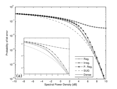
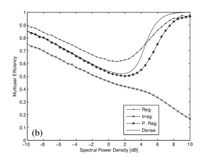
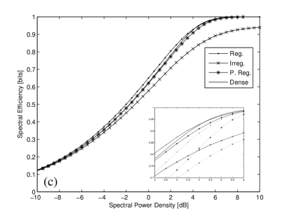
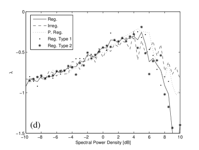
Figure 2: Performance of the sparse CDMA configuration of variable and factor degree connectivities $C:L=3:3$, respectively; all data presented on the basis of 100 runs, error bars are omitted and are typically small in subfigures (a)-(c) the smoothness of the curves being characteristic of this level (numerical accuracy was excellent only at intermediate $PSD$s). (a) The bit error rate is limited by the disconnected component in the case of irregular codes, otherwise trends match the dense case, lower bounded by the SUG. Inset - the range where the sparse-regular and dense cases crossover.(b) Multiuser efficiency indicates the regular user connectivity codes outperform the dense case below some $PSD$. (c) The spectral efficiency [——] demonstrates similar trends, the entropy being positive. The gap between the mutual information [${\mathinner{\cdotp\cdotp\cdotp\cdotp\cdotp\cdotp}}$] and spectral efficiency (shown in the inset) is everywhere small and especially so at small and large $PSD$, indicating little information loss in the decoding process. (d) The two markers show the mean results for the two different stability estimates in the algorithm for the regular code. There are systematic errors at small $PSD$, and convergence is good only at intermediate $PSD$. The lines represent the average of these quantities for each ensemble – all ensembles show a cusp at some $PSD$, for $3:3$ codes the various ensembles shows very similar trends, indicating local stability everywhere.

Figure 3 indicates the effect of increasing density at fixed $\alpha$ in the case of the regular code. As density is increased the statistics of the sparse codes approach that of the dense channel in all ensembles tested. For the irregular ensemble performance increases monotonically with density at all $PSD$. The rapid convergence to the dense case performance was elsewhere observed for partly regular ensembles, and ensembles based on a Gaussian prior input [2, 7]. At all densities for which single solutions were found the RS assumption appeared validated in the stability parameter and entropy.

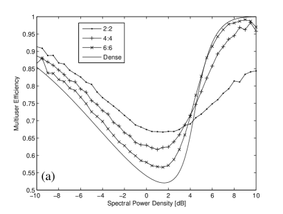
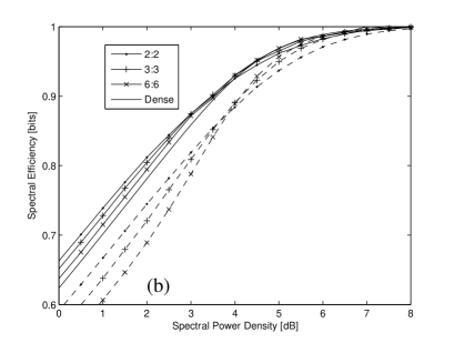
Figure 3: The effect of increasing density for the regular ensemble: (a) Multiuser efficiency, (b) spectral efficiency [——] and mutual information [– – –]. Data presented on the basis of 10 runs, error bars are omitted but of a size comparable with the smoothness of the curves. The performance of sparse codes rapidly approaches that of the dense code everywhere. The $PSD$ threshold beyond which the dense code outperforms the sparse code is fairly stable.

Figure 4 indicates the effect of channel load $\alpha$ on performance. We first explain results for codes in which only a single solution was found (no solution coexistence). For small values of the load a monotonic increase in the bit error rate, and capacity are observed as $\alpha$ is increased with $C$ constant, as shown in figures 4(a) and  4(b), respectively. This matches the trend in the dense case, the dense code becoming superior in performance to the sparse codes as $PSD$ increases. We found that for all sparse ensembles there existed regimes with $\alpha>1.49$ for which only a single stable solution existed, although the equivalent dense systems are known to have two stable solutions in some range of $PSD$ [3]. In all single valued regimes we observed positive entropy, and a negative stability parameter. However, in cases of large $\alpha$ many features became more pronounced close to the dense case solution coexistence regime: notably the cusp in the stability parameter, gap between $MI$ and $\nu$ and the gradient in $P_{b}$.

4.1 Solution Coexistence Regimes

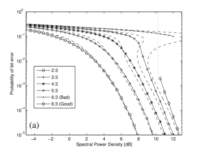
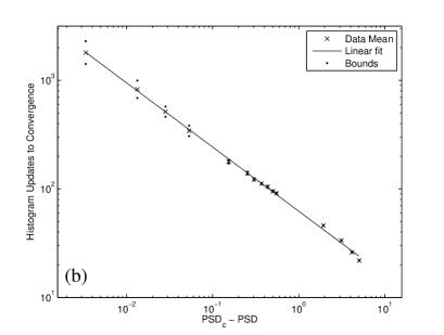
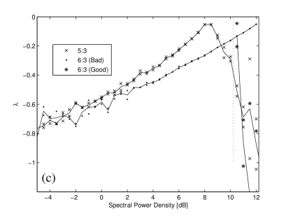
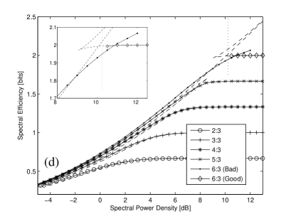
Figure 4: The effect of channel load $\alpha$ on performance for the regular ensemble. Data presented on the basis of 10 runs, error bars omitted but characterised by the smoothness of curves. Dashed lines indicate the dense code analogues. The vertical dotted line indicates the point beyond which $6:3$ random and ferromagnetic initial conditions failed to converge to the same solution, both dynamically stable solutions are shown beyond this point. (a) There is a monotonic increase in bit error rate with the increasing load. (b) Investigation of the $6:3$ code ($\alpha=2$) indicates a divergence in convergence time as $PSD\rightarrow 10.23dB$ with exponent $0.59$ based on a simple linear regression of 15 points (each point is the mean of 10 independent runs). Beyond this point different initial conditions give rise to one of two solutions. (c) The stability parameter was found to be negative for all convergent solutions, indicating the suitability of RS. Where the solution is near ferromagnetic the stability measure becomes quickly very noisy (as shown for the $5:3$ and $6:3$ codes). (d) As load $\alpha$ is increased there is a monotonic increase in capacity. The spectral efficiency for the ’bad’ solution exceeds 2 in a small interval (equivalent to negative entropy), similar to the behaviour reported for the dense case.

As in the case of dense CDMA [3], also here we observe a regime where two solutions, of quite different performance, coexist. In order to investigate the regime where two solutions coexist we investigated the states arrived at from random and ferromagnetic initial conditions (giving bad and good solutions respectively). Separate heuristic convergence criteria were found for the histograms, and these seemed to work well for the good solution. For the bad solution we simply present results after a fixed number of histogram updates ($500$) as all convergence criteria tested appeared either too stringent, to require experimentally inaccessible timescales, or did not capture the asymptotic values for important quantities like entropy. We believe $500$ updates to be sufficiently conservative to capture the properties of these solutions however.

Figure 4(a) shows the dependence of the bit error rate on the load, which is also equivalent to $L/C$. There is a monotonic increase in bit error rate with the load and the emergence and coexistence of two separate solutions above a certain point; in the case of the $6:3$ code the point above which the two solutions coexist is $PSD=10.23dB$ as indicated by the vertical dotted line.

We use the regular code $6:3$ to demonstrate the solution coexistence found above some $PSD$ in various codes. The onset of the bimodal distribution can be identified by the divergence in the convergence time in the single solution regime (the time for the ferromagnetic and random histograms to converge to a common distribution). The time for this to occur, in a heuristically chosen statistic and accuracy, is plotted in figure 4(b). By a naive linear regression across 3 decades we found a power law exponent of $0.59$ and a transition point of $PSD=10.23dB$, but cannot provide a goodness of fit measure to this data. This would represent the point at which at least two stable solutions co-exist.

Beyond $PSD\approx 12dB$ only one stable solution is found from both random and ferromagnetic initial conditions, corresponding statistically to a continuation of the good solution. A solution which statistically resembles a continuation of the bad solution is occasionally arrived at from both initial conditions, this solution had a positive stability parameter and negative entropy – so is not a viable solution. Thus we predict a second dynamical transition in the region of $12dB$, as might be guessed by comparison with the dense case and observation of the trend in the stability parameter (see figure 4(c)).

The stability results are presented in figure 4(c). Only two stable solutions were found in the region beyond this critical point and upto $12dB$, which we infer to be viable RS solutions (where entropy is positive). The bad solution upto 12dB has a well resolved negative value. The good solution has a negative value in its mean, but like other near ferromagnetic solutions investigated results are very noisy due to numerical issues relating to histogram resolution.

Both capacity and spectral efficiency monotonically increase with the load as shown in figure 4(d). For the $6:3$ code we see a separation of the two solutions at $PSD=10.23dB$ (vertical dotted line.) The dashed lines correspond to a similar behaviour observed in the dense case (the range of interest is magnified in the inset.) A cross over in the entropy of the two distinct solutions, near $PSD\approx 11dB$, is indicative of a second order phase transition. As in the dense case, only the solution of smallest spectral efficiency is thermodynamically relevant at a given $PSD$, although the other is likely to be important in decoding dynamics. The trends in the sparse case follow the dense case qualitatively, with the good solution having performance only slightly worse than the corresponding solution in the dense case (and vice versa for the bad solution).

The entropy of the bad solution becomes negative in a small interval (spectral efficiency exceeds 2) although no local instability is observed. The static and dynamic properties of the histograms appear to be well resolved in this region. However, the negative entropy indicates an instability towards either a type of solution not captured within the RS assumption, or towards some metastable configuration. We will not speculate further, the bad solution is in any case thermodynamically subdominant in its low and negative entropy form.

Our hypothesis is therefore that the trends in the sparse ensembles match those in the dense ensembles within the coexistence region and $RS$ continues to be valid for each of two distinct positive entropy solutions. The coexistence region for the sparse codes is however smaller than in the corresponding dense ensembles. Since our histogram updates mirror the properties of a belief propagation algorithm on a random graph we can suspect that the bad solution may have implications for the performance of belief propagation decoding in the coexistence region, and that convergence problems will appear near this region. In the user regular codes investigated the bad solution of the sparse ensemble outperforms the bad solution of the dense ensemble, and vice-versa for the good solution. Thus regardless of whether sparse decoding performance is good or bad, the dynamical transition point for the dense ensemble would corresponds to a $PSD$ beyond which dense CDMA outperforms sparse CDMA at a particular load.

4.2 Spectral Efficiency Lower Bound Numerical Results

Finally we present figure 5, which shows the the mutual information between a single chip and transmitted bits for sparse ensembles of differing chip connectivity in the infinite $PSD$ (zero noise) limit (15). This shows that in expectation a chip drawn from the regular ensemble contains more information on the transmitted bits than a chip drawn from any other ensemble (including the Poissonian ensemble). The difference between the regular and Poissonian ensembles becomes relatively smaller as $L$ increases. This appears consistent with the replica method results found at high $PSD$, although regular chip connectivity under performed by comparison with Poisson distributed chip connectivity in the low $PSD$ regime, which was not anticipated by the single chip approximation.

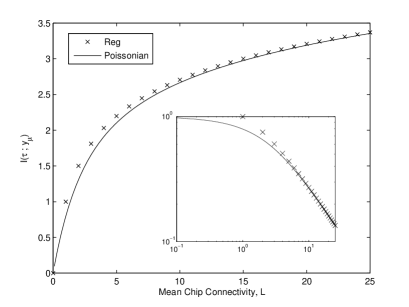
Figure 5: A $PSD\rightarrow\infty$ limit to the expected mutual information between a single chip, and the transmitted bits. Mutual Information is highest for regular chip connectivities, with the Poissonian chip connectivity result also shown, the discrepancy becoming relatively small as $L$ increases. The inset shows the mutual information/bit decoded ($\left\langle I(\mbox{\boldmath{$\tau$}};y_{\mu})\right\rangle/L$) on a log-log plot to demonstrate an asymptotic power law behaviour and show more detail in the cases of small $L$.

5 Concluding Remarks

Our results demonstrate the feasibility of sparse regular codes for use in CDMA. At moderate $PSD$ it seems the performance of sparse regular codes may be very good. With the replica symmetric assumption apparently valid at practical $PSD$ it is likely that fast algorithms based on belief propagation may be very successful in achieving the theoretical results. Furthermore for lower density sparse codes the problem of the coexistence regime, which limits the performance of practical decoding methods, seems to be less pervasive than for dense ensembles in the over saturated regime.

A direct evaluation of the properties of belief propagation may prove similar results to those shown here. In the absence of replica symmetry breaking states it is normally true that belief propagation performs very well. However, to make best use of the channel resources it may be preferable to implement high load regimes in cases of high $PSD$, and so overcoming the algorithmic problems arising from the solution coexistence is a challenge of practical importance in this case.

Other practical issues in implementation are certainly significant. Similar to the case of dense CDMA there are considerable problems relating to multipath, fading and power control, in fact it is known that these effects are more disruptive for the sparse codes, especially regular codes. However, certain situations such as broadcasting (one to many) channels and downlink CDMA, where synchronisation can be assumed, may be practical points for future implementation. There are practical advantages of the sparse case over dense and orthogonal codes in some regimes. The sparse CDMA method is likely to be particularly useful in frequency-hopping and time-hopping code division multiple access (FH and TH -CDMA) applications where the effect of these practical limitations is less emphasised.

Extensions based on our method to cases without power control or synchronisation have been attempted and are quite difficult. A consideration of priors on the inputs, in particular the effects when sparse CDMA is combined with some encoding method may also be interesting.

Bibliography

Bibliography

- [1] S. Verdu. Multiuser Detection. Cambridge University Press, New York, NY, USA, 1998.
- [2] M. Yoshida and T. Tanaka. Analysis of sparsely-spread cdma via statistical mechanics. In Proceedings - IEEE International Symposium on Information Theory, 2006., pages 2378–2382, 2006.
- [3] T. Tanaka. A statistical-mechanics approach to large-system analysis of cdma multiuser detectors. Information Theory, IEEE Transactions on, 48(11):2888–2910, Nov 2002.
- [4] D. Guo and S. Verdu. Communications, Information and Network Security, chapter Multiuser Detection and Statistical Mechanics, pages 229–277. Kluwer Academic Publishers, 2002.
- [5] H. Nishimori. Statistical Physics of Spin Glasses and Information Processing. Oxford Science Publications, Oxford, UK, 2001.
- [6] M. Mezard, G. Parisi, and M.A Virasoro. Spin Glass Theory and Beyond. World Scientific, Singapore, 1987.
- [7] A. Montanari and D. Tse. Analysis of belief propagation for non-linear problems: The example of cdma (or: How to prove tanaka’s formula). In Proceedings IEEE Workshop on Information Theory, 2006.
- [8] Y. Kabashima. A statistical-mechanical approach to cdma multiuser detection: propagating beliefs in a densely connected graph. cond-mat/0210535, 2002.
- [9] J.P Neirotti and D. Saad. Improved message passing for inference in densely connected systems. Europhys. Lett., 71(5):866–872, 2005.
- [10] A. Montanari, B. Prabhakar, and D. Tse. Belief propagation based multiuser detection. In Proceedings of the Allerton Conference on Communication, Control and Computing, Monticello, USA, 2006.
- [11] D. Guo and C. Wang. Multiuser detection of sparsely spread cdma. (unpublished), 2007.
- [12] T. Tanaka and D. Saad. A statistical-mechanical analysis of coded cdma with regular ldpc codes. In Proceedings - IEEE International Symposium on Information Theory, 2003., page 444, 2003.
- [13] D.J. MacKay. Information Theory, Inference and Learning Algorithms. Cambridge University Press, 2004.
- [14] J. Raymond and D. Saad. Randomness and metastability in cdma paradigms. arXiv:0711.4380, 2007.
- [15] R. Vicente, D. Saad, and Y. Kabashima. Advances in Imaging and Electron Physics, volume 125, chapter Low Density Parity Check Codes - A statistical Physics Perspective, pages 231–353. Academic Press, 2002.
- [16] M Talagrand. The generalized parisi formula. Comptes Rendus Mathematique, 337(2):111–114, 2003.
- [17] S. Franz, M. Leone, and F.L. Toninelli. Replica bounds for diluted non-poissonian spin systems. Journal of Physics A: Mathematical and General, 36(43):10967–10985, 2003.
- [18] F. Guerra. Broken Replica Symmetry Bounds in the Mean Field Spin Glass Model. Communications in Mathematical Physics, 233:1–12, 2003.
- [19] R. Monasson. Optimization problems and replica symmetry breaking in finite connectivity spin glasses. J. Phys. A, 31(2):513–529, 1998.
- [20] K.Y.M. Wong and D. Sherrington. Graph bipartitioning and spin-glasses on a random network of fixed finite valence. J. Phys. A, 20:L793–99, 1987.
- [21] M. Mezard and G. Parisi. The bethe lattice spin glass revisited. Euro. Phys. Jour. B, 20(2):217–233, 2001.
- [22] O. Rivoire, G. Biroli, O.C. Martin, and M. M zard. Glass models on bethe lattices. Euro. Phys. J. B, 37:55–78, 2004.
- [23] Y. Kapashima. Propagating beliefs in spin glass models. J. Phys. Soc. Jpn., 72:1645–1649, 2003.
- [24] J. Raymond, A. Sportiello, and L. Zdeborov . The phase diagram of random 1-in-3 satisfiability problem. Phys. Rev. E., 76(1):011101, 2007.