[0704.0070] Coincidence of the oscillations in the dipole transition and in the persistent current of narrow quantum rings with two electrons

* The corresponding author

Quantum rings containing only a few electrons can be now fabricated in laboratories ${}^{1,2}.$ When a magnetic field $B$ is applied, interesting physical phenomena, e.g., Aharonov-Bohm oscillation (ABO) and fractional ABO (FABO)of the ground state (GS) energy $E_{o}$ and persistent current $J_{o}$ , have been observed ^2-4,13. In the theoretical aspect, a number of calculations based on exact diagonalization^5-8, local-spin-density approximation^9,10, and the diffusion Monte Carlo method¹¹ have been performed. These calculations can in general reproduce the experimental data. For examples, in the calculation of 4-electron ring^6,11, the period of oscillation $\Phi_{0}/4$ found in experiments was recovered $(\Phi_{0}=hc/eisthefluxquantum)$ .

In addition to the oscillations in $E_{o}$ and $J_{o}$ , the oscillation in the optical properties is noticeable.^16,17. In this paper a new kind of oscillation found in the dipole transition of two-electron (2-e) narrow rings is reported. The emitted (absorbed) photon of the dipole transition of the GS was found to have essentially two energies, their difference is exactly equal to $hJ_{o}$ , where $h$ is the Planck’s constant. In other words the difference of the two photon energies appears as an oscillation which matches exactly the oscillation of $J_{o}$ . This finding is approved by both numerical calculation and analytical analysis as follows.

The narrow 2-e ring is first considered as one-dimensional, then the effect of the width of the ring is further evaluated afterward. The Hamiltonian reads

$H=T+V_{12}+H_{Zeeman}\qquad\qquad(1)$

$T=\sum\limits_{j=1}^{N}G(-i\frac{\partial}{\partial\theta_{j}}+\Phi)^{2},\;\;\;G=\frac{\hbar^{2}}{2m^{\ast}R^{2}}$

where $m^{\ast}$ the effective mass, $\theta_{j}$ the azimuthal angle of the $j-th$ electron, $\Phi=\pi R^{2}B/\Phi_{0}$ , where $B$ is a magnetic field perpendicular to the plane of the ring, $V_{12}$ the e-e Coulomb interaction, $H_{Zeeman}=-S_{Z}\mu\Phi$ the well known Zeeman energy where $S_{Z}$ is the Z-component of the total spin $S$ , and $\mu=\frac{g^{\ast}\mu_{B}}{\pi R^{2}\Phi_{0}}$ , where $g^{\ast}$ is the effective g-factor and $\mu_{B}$ is the Bohr magneton. The interaction is adjusted as ⁷ $V_{12}=e^{2}/({2\varepsilon\sqrt{d^{2}+R^{2}\sin^{2}((\theta_{1}-\theta_{2})/2)}})^{-1}$ , where $\varepsilon$ is the dielectric constant and the parameter $d$ is introduced to account for the effect of finite thickness of the ring.

We first perform a numerical calculation so that all related quantities can be evaluated quantitatively. $m^{\ast}=0.063m_{e}$ , $\varepsilon=12.4$ (for InGaAs), $d=0.05R$ , and the units $meV$ , $nm$ , $Tesla$ and $\Phi_{0}$ are used. Accordingly, $G=604.8/R^{2},$ and $\mu=33.53/R^{2}$ .

A set of basis functions $\phi_{k_{1}k_{2}}=e^{i(k_{1}\theta_{1}+k_{2}\theta_{2})}/2\pi$ is introduced to diagonalize the Hamiltonian, where $k_{1}$ and $k_{2}$ must be integers to assure the periodicity, the sum of $k_{1}$ and $k_{2}$ is just the total orbital angular momentum $L$ . $\phi_{k_{1}k_{2}}$ must be further (anti-)symmetrized when $S=0(1)$ . When about three thousand basis functions are adopted, accurate solutions (at least six effective digits) can be obtained. The low-lying spectrum is plotted in Fig.1, where the oscillation of the GS energy and the transition of the GS angular momentum $L_{o}$ can be clearly seen.

Let $\theta_{C}=(\theta_{2}+\theta_{1})/2$ , and $\varphi=\theta_{2}-\theta_{1}$ . Then

$H=H_{coll}+H_{int}\qquad\qquad(2)$

where $H_{coll}=\frac{1}{2}G(-i\frac{\partial}{\partial\theta_{C}}+2\Phi)^{2}+H_{Zeeman}$ and $H_{int}=2G(-i\frac{\partial}{\partial\varphi})^{2}+V_{12}$ , they are for the collective and internal motions, respectively. Our numerical results lead to the following points.

(i) Separability: The separability of one-dimensional ring is well known⁵. However, for the convenience of the following description, it is briefly summarized as follows. Each eigenenergy $E$ can be exactly divided as a sum of three terms

$E=\frac{1}{2}G(L+2\Phi)^{2}+E_{int}-S_{Z}\mu\Phi\qquad\qquad(3)$

where the first term is the kinetic energy of collective motion, $E_{int}$ is the internal energy .

Since the basis functions can be rewritten as

$\phi_{k_{1}k_{2}}=e^{iL\theta_{C}}e^{i\frac{1}{2}(k_{2}-k_{1})\varphi}/2\pi\qquad\qquad(4)$

the spatial part of each eigenstate $\Psi$ is strictly separable as $\Psi=\frac{1}{\sqrt{2\pi}}e^{iL\;\theta_{C}}\psi_{int}$ where the first part describes the collective motion, while $\psi_{int}$ is a normalized internal state depending only on $\varphi$ . In particular, both $E_{int}$ and $\psi_{int}$ do not depend on $B$ (or $\Phi$ ).

(ii) Classification of $\psi_{int}$ : When $L$ is even (odd), $(k_{2}-k_{1})/2$ is an integer (half-integer), thus the period of $\varphi$ as shown in (4) is $2\pi\;(4\pi)$ . Therefore, the periodicity of the internal states have two choices. In fact, the difference in the periodicity is closely related to the dependence of the domains of the new variables $\theta_{C}$ and $\varphi$ , this point has been discussed in detail in ref.[14,15]. Let $Q=(-1)^{L}$ , then the four cases $(Q,S)=$ (1,0), (-1,0), (-1,1) and (1,1) are associated with four types of states labeled by $a,\;b,\;c,$ and $d$ , respectively. The internal states of Type $a$ are denoted as $\psi_{a}$ , $\psi_{a^{\ast}}$ , $\cdot\cdot\cdot$ and the associated internal energies as $E_{a}<E_{a^{\ast}}$ , $\cdot\cdot\cdot$ and so on. Examples of $\psi_{int}$ and $E_{int}$ are plotted in Fig.2 and listed in Table 1, respectively.

Table 1, The lowest and second lowest internal energies (in $meV$ ) of Type $a$ to $d$ , $R=30nm.$

Type	$a$	$b$	$c$	$d$
$E_{int}$	$2.626$	$4.247$	2.630	4.272
$E_{int}^{\ast}$	$6.342$	$8.912$	6.435	9.158

Due to the e-e repulsion, a dumbbell shape (DB), i.e., $\varphi=180^{\circ}$ , is advantageous in energy because the two electrons are farther away from each other meanwhile. However, a rotation of this geometry by $\pi$ is equivalent to an interchange of particles, these operations will create the factors $(-1)^{L}$ and $(-1)^{S}$ , respectively, from the wave function. Therefore, the equivalence leads to a constraint, accordingly the DB is allowed only for the states with $L+S$ even, i.e., only for Type $a$ and $c$ . Otherwise, the states would have an inherent node at the DB and therefore be higher in energy as shown in Table 1, where $E_{a}<<E_{b}$ , $E_{c}<<E_{d}$ , and $E_{a}\approx E_{c}$ . In Fig.2 the patterns of Type $a$ are one-to-one similar to Type $c$ , they all have a peak at the DB. On the contrary, all those of Type ( $b$ ) and( $d$ ) have the inherent node at the DB. It is noticeable that Type $b$ and $c$ are not continuous at $\varphi=0$ and $2\pi$ due to their periods are not equal to $2\pi$ . It was found that the internal states of all the GSs are either $\psi_{a}$ or $\psi_{c}$ without exceptions because the favorable DB is allowed in them. When the dynamical parameters vary in reasonable ranges, the qualitative features of Fig.2 remain the same.

According to (3), an appropriate $L_{o}$ would be chosen to minimize the GS energy. When $\Phi$ increases, $L_{o}$ will undergo even-odd transitions repeatedly and become more negative as shown in Fig.1. Correspondingly, the total spin $S_{o}$ undergoes singlet-triplet transitions, and $\psi_{a}$ and $\psi_{c}$ appear in the GS alternatively. However, due to the Zeeman effect, when $\Phi$ is larger than a critical value $\Phi_{crit}$ , only $S_{o}=1$ states will be dominant, and accordingly only $\psi_{c}$ will appear in the GS. The region $\Phi<(>)\;\Phi_{crit}$ is called the FABO (ABO) region.

(iii) Persistent Current: Let $J_{1}$ be the current of the particle $e_{1}$ . The expression of $J_{1}$ is well known.⁵ However, since it does not depend on the azimuthal angle, it equals to its average over $\theta_{1}$ . Thus the total current $J=J_{1}+J_{2}$ is

$J=\frac{1}{4\pi}g\int d\theta_{1}d\theta_{2}\;[\Psi^{\ast}(-i\frac{\partial}{\partial\theta_{1}}-i\frac{\partial}{\partial\theta_{2}}+2\Phi)\Psi+c.c.]\ \ \ \ \ (5)$

where $g=\hbar/(m^{\ast}R^{2})$ . Using the arguments $\theta_{C}$ and $\varphi$ and making use of the separability, the integration over $\theta_{C}$ and $\varphi$ can be performed. Thus we have

$J=g(L+2\Phi)/2\pi\qquad\qquad\qquad(6)$

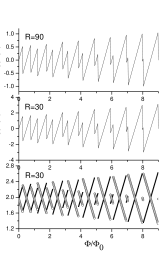
This equation demonstrates explicitly the mechanism of the oscillation of the persistent current, it is caused by the step-by-step transition of $L$ during the increase of $\Phi$ . Examples of $J$ are shown in Fig.3, where each stronger oscillation (associated with a $L$ odd and $S=1$ GS) is followed by a weaker oscillation (associated with a $L$ even and $S=0$ GS).

(iv) Relations among the internal states: Define

$O_{m}=e^{im(\theta_{1}-\theta_{C})}+$ $e^{im(\theta_{2}-\theta_{C})}=2\cos(m\varphi/2)$ . By analyzing the numerical data, we found

$\tilde{N}(O_{1}\psi_{a})=\psi_{b}+\xi_{a}$ and $\tilde{N}(O_{1}\psi_{c})=\psi_{d}+\xi_{c}\qquad(7)$

where $\tilde{N}$ is the operator of normalization, both $\xi_{a}$ and $\xi_{c}$ are very small functions and depend on the dynamical parameters very weakly. E.g., when $R$ varies from 30 to 90, the weights of $\xi_{a}$ and $\xi_{c}$ vary from $0.0004$ to $0.0002$ . They are so small that in fact can be neglected. Since $O_{1}$ contains a node at the DB, it must cause a change of type from $a$ to $b$ , or from $c$ to $d$ . Thus it is not surprising that (7) holds. Since $O_{1}$ is the operator of the dipole transition (see below), eq.(7) provides an additional rule of selection as discussed later.

(v) Dipole transition: The probability of dipole transition reads $P_{(o),\pm}^{(f)}=\frac{2e^{2}}{3\hbar}\;(\omega_{\pm}/c)^{3}R^{2}\;|A_{(o),\pm}^{(f)}|^{2}$ , where $\omega_{\pm}$ is the frequency of the photon,

$A_{(o)}^{(f)\pm}=\langle\Psi_{(f)\pm}|e^{\pm i\theta_{1}}+e^{\pm i\theta_{2}}|\Psi_{(o)}\rangle$

$=\delta_{L_{(f)},\;L_{(o)}\;\pm 1}\langle\psi_{int}^{(f)\pm}|O_{1}|\psi_{int}^{(o)}\rangle$ (8)

where $(f)$ and $(o)$ denote the final and initial states, respectively, the signs $\pm$ are associated with $L_{(f)}=L_{(o)}\;\pm 1$ .

Let the initial state be the GS with $L_{o}$ , then $\psi_{int}^{(o)}$ must be $\psi_{a}$ or $\psi_{c}$ depending on $L_{o}$ is even or odd . Let $\alpha$ denotes the type of the initial state. Due to (7) , $\langle\psi_{int}^{(f)\pm}|O_{1}|\psi_{int}^{(o)}\rangle=\delta_{(f),\alpha}<O_{1}\psi_{\alpha}|O_{1}\psi_{\alpha}>^{1/2}$ , where $\delta_{(f),\alpha}$ implies that the final state must be $\psi_{b}$ ( $\psi_{d}$ ) if $\alpha=a$ ( $c$ ), otherwise the amplitude is zero. Thus, due to the additional rule of selection eq.(7), the dipole strength of the GS is completely concentrated in two final states having $L_{(f)}=L_{(o)}\;\pm 1$ and both having the same internal state specified by eq.(7). Accordingly, only the photons with the two energies

$\hbar\omega_{\pm}=E_{(f)\pm}-E_{(o)}$

$=G[\frac{1}{2}(1\pm 2(L_{o}+2\Phi))+\Delta_{\alpha}/G]$ (9)

can be emitted (absorbed), where $\Delta_{\alpha}=E_{b}-E_{a}$ or $E_{d}-E_{c}$ depending on $\alpha=a$ or ( $c$ ). The oscillation of $\hbar\omega_{\pm}$ is plotted in the lowest panel of Fig.3. It turns out that $\Delta_{\alpha}/G$ depends on $R$ very weakly, thus $\hbar\omega_{\pm}$ is nearly proportional to $R^{-2}$ . Accordingly, a smaller ring will have a larger probability of transition with a higher energy.

(vi) FABO region: The oscillation in this region is complicated as shown in Fig.1 and 3. It is noted that the GS energy (3), persistent current (6), and the photon energies (9) all contain the factor $L_{o}+2\Phi,$ thus their FABO are completely in phase and have the same mechanism caused by the transition of $L_{o}$ against $\Phi$ . In Fig.1 the abscissa $\Phi$ can be divided into segments, in each the GS has a specific $L_{o}$ and the GS energy is given by a piece of a parabolic curve. The segment is called an even (odd) segment if $L_{o}$ is even (odd). At the border of two neighboring segments the two GS energies are equal. From the equality and based on (3), the right and left boundaries of the segment with $L_{o}$ can be obtained as

$\Phi_{right}(L_{o})=(1-(\mu/2G)^{2})^{-1}[\;1-\mu(E_{c}-E_{a})/G^{2}-2L_{o}+(-1)^{L_{o}}(2(E_{c}-E_{a})+\mu(L_{o}-1/2))/G]/4\qquad\qquad(10)$

$\Phi_{left}(L_{o})\;=(1-(\mu/2G)^{2})^{-1}[-1-\mu(E_{c}-E_{a})/G^{2}-2L_{o}-(-1)^{L_{o}}(2(E_{c}-E_{a})+\mu(L_{o}+1/2))/G]/4\qquad(11)$

where $L_{o}\leq 0$ and $\Phi_{right}(L_{o})=\Phi_{left}(L_{o}-1)$ , $\mu$ arises from the $H_{Zeeman}$ . The length of the segment reads

$d_{L_{o}}=\Phi_{right}(L_{o})-\Phi_{left}(L_{o})=(1-(\mu/2G)^{2})^{-1}[1+(-1)^{L_{o}}(2(E_{c}-E_{a})+\mu L_{o})/G]/2\qquad\qquad\qquad(12)$

which is related to the period of the FABO. When $\Phi$ increases, the magnitude of $L_{o}$ would increase. Since $\mu L_{o}$ is negative, it is clear from eq.(12) that the length of even (odd) segments would become shorter (longer) when $\Phi$ increases.

The location of a segment with a given $L_{o}$ can be known from the inequality $\Phi_{left}(L_{o})\leq\Phi\leq\Phi_{right}(L_{o})$ . Once the relation between $L_{o}$ and the segments of $\Phi$ is clear, every details of the FABO can be analytically and exactly explained via the eq.(3), (6), and (9). In particular, the extrema in each segment can be known by giving $\Phi=\Phi_{right}$ or $\Phi_{left}$ . For an example, the maximal current is $g(L_{o}+2\Phi_{right})/2\pi$ . Incidentally, the minimum of the GS energy in a segment is $E_{\min}=E_{c}-\mu^{2}/8G+\mu L_{o}/2$ (if $S_{o}=1$ ), or just equal to $E_{a}$ (if $S_{0}=0$ ).

It is noted that $E_{c}-E_{a}$ (cf. Table 1) and $\mu/G$ (it is $0.0554$ in our case) are both small. When $\Phi$ is small the magnitude of $|L_{o}|$ would be also small . In this case eq.(12) leads to $d_{L_{o}}\approx 1/2$ , i.e., the period is a half of the one of the normal ABO. In fact, (12) provides an quantitative description of the variation of the period of the FABO.

(vii) ABO region: When $\Phi$ becomes sufficiently large, $L_{o}$ will become very negative, the even segments will disappear due to their lengths $d_{L_{o}}\leq 0$ . We can define a critical odd integer $L_{crit}$ so that $d_{L_{crit}-1}\leq 0$ while $d_{L_{crit}+1}>0$ , thereby the critical flux separating the FABO and ABO region can be defined as

$\Phi_{crit}=\Phi_{left}(L_{crit})\qquad\qquad(13)$

Once $\Phi>\Phi_{crit}$ , $L_{o}$ remains odd and the system keeps polarized. Let $I_{X}$ be the largest even integer smaller than $-(G+2(E_{c}-E_{a}))/\mu$ . It turns out from eq.(12) that $L_{crit}=I_{X}+1$ . With our parameters, $L_{crit}=-19$ and accordingly $\Phi_{crit}=9.003$ ( refer to Fig.1). Both $L_{crit}$ and $\Phi_{crit}$ depend on $R$ very weakly, but sensitively on the effective mass $m^{\ast}$ .

In the ABO region ( $\Phi>\Phi_{crit}$ ), eqs.(10) to (12) do not hold. Instead we have $\Phi_{right}=-(L_{o}-1)/2,\;\Phi_{left}=-(L_{o}+1)/2,$ and $d_{L_{o}}=1$ . Thus the normal ABO recovers. Evaluated from (6), the magnitude of current is from $-g/2\pi$ to $g/2\pi$ (for a comparison, it is from $-g/4\pi$ to $g/4\pi$ for 1-e rings). From (9) the photon energies $\hbar\omega_{+}$ is from $\Delta_{c}-G/2$ to $\Delta_{c}+3G/2$ , at the same time $\hbar\omega_{-}$ is from $\Delta_{c}+3G/2$ to $\Delta_{c}-G/2$ .

(viii) Relations between the photon energies and other physical quantities: Due to (7), the emitted (absorbed) dipole photon has only two frequencies , therefore it is meaningful to define $\Delta_{\hbar\omega}=\hbar(\omega_{+}-\omega_{-})$ . Directly from (9) and (6), we have

$\Delta_{\hbar\omega}=hJ_{o}\qquad\qquad(14)$

where $h$ is the Planck’s constant and $J_{o}$ is the persistent current of the GS. To compare with 1-e rings, the latter has $\Delta_{\hbar\omega}=2hJ_{o}$ Ėq.(14) demonstrates that the oscillation of $\Delta_{\hbar\omega}$ and the oscillation of $J_{o}$ are matched with each other exactly, they keep strictly proportional to each other during the variation of $\Phi$ .

The maxima of $\Delta_{\hbar\omega}$ measured in the ABO and FABO regions, respectively, read

$(\Delta_{\hbar\omega})_{\max}^{AB}=2G\qquad\qquad(15)$

$(\Delta_{\hbar\omega})_{\max}^{FAB}=2G(L_{o}+2\Phi_{right})\qquad\qquad(16)$

Obviously, (15) provides a way to determine $G$ , $m^{\ast}$ can be thereby obtained. (16) can be rewritten as

$E_{c}-E_{a}=(G-\mu L_{o})/2-(2G-\mu)/(4G)(\Delta_{\hbar\omega})_{\max}^{FAB}\ \ \ (17)$

This equation can be used to determine $E_{c}-E_{a}$ . Furthermore, we define

$\Gamma_{\hbar\omega}=\hbar(\omega_{+}+\omega_{-})=G+2\Delta_{\alpha}\qquad\qquad(18)$

Once $G$ has been known, (18) can be used to determine $E_{b}-E_{a}$ and $E_{d}-E_{c}$ . Since the spectrum can be generated from the internal energies via (3), the evolutions of the spectrum and the persistent current against $\Phi$ can be understood simply by measuring the photon energies.

(ix) Effect of the width: We now consider a two-dimensional model in which the two electrons are strictly confined in an annular region by a potential $U(r),$ which is zero if $r_{a}<r<r_{b}$ or is infinite otherwise. Under this model we have performed numerical calculation to obtain $\Delta_{\hbar\omega}$ and $hJ_{o}$ , where $J_{o}$ is now the total angular current inside the ring (from $r_{a}$ to $r_{b}$ ). The result is shown in Fig.4 where $r_{a}=50$ and $r_{b}=120$ are assumed, and the two quantities are slightly different from each other. However, when the width becomes smaller, say $r_{b}-r_{a}<30$ , the two curves overlap. Thus (14) works not only for one-dimensional but also for two-dimensional narrow rings. Let us define $\stackrel{{\scriptstyle\_}}{{r}}$ $=\hbar/\sqrt{m^{\ast}(\Delta_{\hbar\omega})_{\max}^{AB}}$ . For one-dimensional rings and from (15), we have $\stackrel{{\scriptstyle\_}}{{r}}=R$ , where $R$ is the radius of the ring. For two-dimensional rings, it was found from our numerical calculation that $\stackrel{{\scriptstyle\_}}{{r}}$ $\approx(r_{b}+r_{a})/2$ if $r_{b}-r_{a}<30$ . E.g., when $r_{b}=100$ and $r_{a}=70$ , $\stackrel{{\scriptstyle\_}}{{r}}$ =85.03. When $r_{b}=100$ and $r_{a}=90$ , $\stackrel{{\scriptstyle\_}}{{r}}$ =95.00. Thus (15) works also well for two-dimensional narrow rings if the $R$ in $G$ is replaced by the average radius.

It is noted that the band-structure and related optical properties of 2-e rings have already been studied in detail by Wendler and coauthors¹⁸. They classify the eigenstates according to their radial motion, relative angular motion, and collective rotation. In our paper the relative angular motion is further classified into four types according to the inherent nodal structures and periodicity of their wave functions, i.e., according to whether the DB shape is allowed and whether the wave function is continuous at $\varphi=2\pi$ . The DB-accessibility turns out to be important because it affects the eigenenergies decisively. In fact, the classification of states based on inherent nodal structures was found to be crucial in atomic physics,¹⁹ this would be also true in two-dimensional systems. Furthermore, the rule of selection for the dipole transition has been proposed in ref.[18]. In our paper, an additional rule (namely,eq.(7)) is further proposed based on the possible transition of internal structures. This rule would affect the dipole spectrum seriously because the emission (absorption) is thereby concentrated into two frequencies. The difference of these two frequencies turns out to be proportional to the persistent current. Therefore the measurement of this difference can be used to determine the magnitude of the current.

In summary, we have studied the FABO both analytically and numerically. The analytical formalism provides not only a base for qualitative understanding, but also provides a number of formulae for quantitative description. The domain of $\Phi$ is divided into segments, each corresponds to a $L_{o}$ . This division describes exactly how $L_{o}$ would transit against $|Phi$ , which causes directly the FABO. Thereby the variation of the period and amplitude of the oscillation of the GS energy, persistent current, and the frequencies of dipole transition in the FABO region can be described exactly. A number of equalities to relate the physical quantities and dynamical parameters have been found. In particular, a new oscillation, namely, the oscillation of $\Delta_{\hbar\omega}$ was found to match exactly the oscillation of $J_{o}$ . Since the photon energies can be more accurately measured, other observables and parameters can be thereby determined via the equalities. Since the separability of the Hamiltonian and the existence of inherent nodes are common, the above description can be more or less generalized to $N-$ electron rings, this deserves to be further studied.

Acknowledgment, This work is supported by the NSFC of China under the grants 10574163 and 90306016.

.REFERENCES

1, A. Lorke, R.J. Luyken, A.O. Govorov, J.P. Kotthaus, J.M. Garcia, and P.M. Petroff, Phys. Rev. Lett. 84, 2223 (2000).

2, U.F. Keyser, C. Fühner, S. Borck, R.J. Haug, M. Bichler, G. Abstreiter, and W. Wegscheider, Phys. Rev. Lett. 90, 196601 (2003)

3, D. Mailly, C. Chapelier, and A. Benoit, Phys. Rev. Lett. 70, 2020 (1993)

4, A. Fuhrer, S. Lüscher, T. Ihn, T. Heinzel, K. Ensslin, W. Wegscheider, and M. Bichler, Nature (London) 413, 822 (2001)

5, S. Viefers, P. Koskinen, P.Singha Deo, M. Manninen, Physica E 21, 1(2004).

6, K. Niemelä, P. Pietiläinen, P. Hyvönen, and T. Chakraborty, Europhys. Lett. 36, 533 (1996)

7, M. Korkusinski, P. Hawrylak, and M. Bayer, Phys. Stat. Sol. B 234, 273 (2002)

8, Z. Barticevic, G. Fuster, and M. Pacheco, Phys. Rev. B 65, 193307 (2002)

9, M. Ferconi and G.Vignale, Phys. Rev. B 50, 14722 (1994).

10, Li. Serra, M. Barranco, A. Emperador, M. Pi, and E. Lipparini, Phys. Rev. B 59, 15290 (1999)

11 A. Emperador, F. Pederiva, and E. Lipparini, Phys. Rev. B 68, 115312 (2003)

12, C.G. Bao, G.M. Huang, Y.M. Liu, Phys. Rev. B 72, 195310 (2005)

13, A.E. Hansen, A. Kristensen, S. Pedersen, C.B. Sorensen, and P.E. Lindelof, Physica E (Amsterdam) 12,770 (2002).

14, K. Moulopoulos and M. Constantinou, Phys. Rev. B. 70, 235327 (2004)

15,J. Planelles, J.I. Climente, and J.L. Movilla, arXiv:cond-mat/0506691 (2005)

16, J.I. Climente and J. Planelles, Phys. Rev. B 72, 155322 (2005)

17, A.O. Govorov, S.E. Ulloa, K. Karrai, and R.J. Warburton, Phys. Rev. B 66, 081309 (2002)

18, L. Wendler, V.M. Fomin, A.V. Chaplik, and A.O. Govorov, Phys. Rev. B 54, 4794 (1996).

19, M.D. Poulsen and L.B. Madsen, Phys. Rev. A 72, 042501 (2005).

Coincidence of the oscillations in the dipole transition and in the persistent current of narrow quantum rings with two electrons

Abstract

pacs: