Order of Epitaxial Self-Assembled Quantum Dots: Linear Analysis

Abstract

Epitaxial self-assembled quantum dots (SAQDs) are of interest for nanostructured optoelectronic and electronic devices such as lasers, photodetectors and nanoscale logic. Spatial order and size order of SAQDs are important to the development of usable devices. It is likely that these two types of order are strongly linked; thus, a study of spatial order will also have strong implications for size order. Here a study of spatial order is undertaken using a linear analysis of a commonly used model of SAQD formation based on surface diffusion. Analytic formulas for film-height correlation functions are found that characterize quantum dot spatial order and corresponding correlation lengths that quantify order. Initial atomic-scale random fluctuations result in relatively small correlation lengths (about two dots) when the effect of a wetting potential is negligible; however, the correlation lengths diverge when SAQDs are allowed to form at a near-critical film height. The present work reinforces previous findings about anisotropy and SAQD order and presents as explicit and transparent mechanism for ordering with corresponding analytic equations. In addition, SAQD formation is by its nature a stochastic process, and various mathematical aspects regarding statistical analysis of SAQD formation and order are presented.

keywords: quantum dots, strained films, epitaxial growth, semiconductors

1 Introduction

Epitaxial self-assembled quantum dots (SAQDs) represent an important step in the advancement of semiconductor fabrication at the nanoscale that will allow breakthroughs in optoelectronics and electronics. [1, 2, 3, 4, 5, 6, 7, 8, 9, 10, 11, 12] Most frequent optoelectronic applications are high efficiency lasers with exotic wavelengths or photodetectors. [1, 3, 4, 5, 6, 7, 8, 10, 11, 12] SAQDs are the result of a transition from 2D growth to 3D growth in strained epitaxial films such as $\mbox{Si}_{x}$$\mbox{Ge}_{1-x}$/Si and $\mbox{In}_{x}\mbox{Ga}_{1-x}\mbox{As}$/GaAs. This process is known as Stranski-Krastanow growth or Volmer-Webber growth. [13, 1, 14, 15].

In applications, order is a key factor. There are two types of order, spatial and size. Spatial order refers to the regularity of SAQD dot placement, and it is necessary for nano-circuitry applications. Size order refers to the uniformity of SAQD size which determines the voltage and/or energy level quantization of SAQDs. It is reasonable to expect that these type of order are linked, and it is important to understand the factors that determine SAQD order. Further understanding should help in the design and simulation of both spontaneous “bottom up” self-assembly and directed or guided self-assembly to enhance SAQD order. [16, 17, 18, 19, 20, 21, 22, 23]Here, an elaboration of and further application of a linear analysis of SAQD order [24] is presented. The work reported here forms the basis of a non-linear theory and modeling of SAQD order that will be reported in future work.

In [24] it was reported that one could calculate a correlation function using a linearized model of SAQD formation. This correlation function included two correlation lengths that could be used to describe SAQD order. It was also found that one effect of a hypothesized wetting potential was to enhance SAQD order when growth occurs near the critical film height for 3D growth. Here, these results are expanded to create a more rigorous linearized theory of SAQD order that will inform non-linear theories. In particular, the model is generalized to any model that combines local energy effects such as surface energy density and non-local elastic destabilization, and the procedure for predicting order based on any linear theory with peak wavelengths is presented. The hypothesized effect of elastic anisotropy in [24] is verified with calculations using linear anisotropic elasticity theory. [25, 26] Details such as statistical fluctuation and convergence are also addressed along with a discussion of the possible forms of linear anisotropic terms in SAQD growth kinetics, and the effect of an atomic-scale cutoff in the continuum theory is addressed. Finally, the order enhancing effect of growing near the critical threshold is explored in more detail using calculations appropriate to Ge/Si SAQDs.

In the literature, two modes of SAQD formation are generally discussed, the thermal nucleation mode and the nucleationless mode. [27, 28, 29] In the thermal nucleation mode, a 2D film surface is metastable, and the formation of individual quantum dots is thermally activated. [27]. This growth mode leads to the formation of individual quantum dots as uncorrelated or loosely correlated discrete events at essentially random locations. In the nucleationless mode, the 2D film surface transitions from stable (or metastable) to unstable. In this mode, dots form everywhere at once appearing at first as a cross-hatched ripple-like disturbance on the 2D film surface and then maturing into recognizable individual dots.[27, 30, 28, 31, 32] These two modes are probably connected via an encompassing conceptual and mathematical model, and perhaps some of what is observed experimentally is in fact a hybrid mechanism. In agreement with intuition, it appears that the nucleationless mode leads to a more ordered dot pattern than the thermal nucleation mode that is dominated by randomness.  Thus, the presented analysis applies to the nucleationless mode.

There are various implementations of nucleationless growth models [28, 37, 38, 39, 40, 18, 34], although, there is also a great deal of commonality among these models. In particular, they all include a non-local elastic effect and local surface energies and/or local wetting energies. Here, a linear analysis of quantum dot order resulting from this class of model is presented. Particular note is taken of the effects of stochastic initial conditions crystal anisotropy in general, elastic anisotropy in particular, and the effect of varying film height as a control parameter as first introduced in [33]. A simple model similar to [28, 37, 38, 40, 18] is presented to produce numerical examples and explore the effects of the average film height. Concurrently, a more abstract and general model is presented and analyzed that includes non-local elastic strain effects, and a local combined surface and wetting energy. The linear model with stochastic initial conditions and deterministic film height evolution will pave the way for more sophisticated analysis involving a non-linear model of stochastic film height evolution.

As previously stated, one of the goals in the present work is to further explore the role of the wetting potential during growth near the stability threshold in film height. A wetting potential has been included in the analysis and simulations in [38, 33, 37, 28]. Although somewhat controversial, the wetting potential plays an important phenomenological role. It ensures that growth takes place in the Stranski-Krastanow mode: that a 3D unstable growth occurs only after a critical layer thickness is achieved, and that a residual wetting layer persists. The physical origins and consequences of the wetting potential are discussed in [41, 28]. The analysis presented here is usable in models that neglect the wetting potential by simply setting it to zero. Another possibility is simply that the wetting potential is simply an approximation to the stabilizing effect of intermixing. [42] That said, if the wetting potential is real, the present analysis shows that it is beneficial to SAQD order to grow near the critical layer thickness.

The presented analytic formulas and linear analysis are intended to complement existing numerical models of SAQD order. [43, 37, 44, 45] and to form a basis for future non-linear analytic analysis of SAQD order. The current findings agree with previous work on the beneficial effects of elastic anisotropy to enhance in-plane order.

The linear analysis, of course, represents a simplification of the film evolution, and it applies only to the initial stages of SAQD formation when the nominally flat film surface becomes unstable and transitions to three-dimensional growth. However, the small surface fluctuation stage of SAQD growth determines the initial seeds of order or disorder in an SAQD array; thus, the small fluctuation stage should have an important influence on the final outcome. At later stages when surface fluctuations are large, there is a natural tendency of SAQDS to either order or ripen [33, 37, 46, 39, 47] Ordering systems tend to evolve slowly due to critical slowing down [39], while ripening tends to diminish order further. [37] Thus, it is possible that the linear model could, in fact, yield good predictions of SAQD order. The simplification and linearizion facilitates the development of analytic solutions that are most transparent, easily portable to multiple material systems and have no effective limit on system size. Finally, it is virtually impossible to have a thorough understanding of the full non-linear model without first having a thorough understanding of the linear behavior.

The remainder of the paper is organized as follows. Section 2 presents the physical assumptions and mathematical approximations used to model film growth. Section 3 discusses the stochastic initial conditions and the resulting correlation functions and correlation lengths. Section 4, presents a procedure for estimating SAQD order with an application to Ge dots on a Si substrate. Section 5 presents conclusions, while Appendices A-F present additional calculational details.

2 Modeling

The formation of SAQDs is modeled as a deterministic surface diffusion process with stochastic initial conditions. The resulting equations and ultimately the sought after correlation functions are different depending on whether the film surface is treated as one-dimensional isotropic, two-dimensional isotropic or two-dimensional anisotropic. The 1D and 2D isotropic cases are discussed first, and then the essential differences of the 2D anisotropic model are presented. The stochastic initial conditions need to be expressed in terms of the correlation functions that are also use to analyze order; consequently, the discussion of the initial conditions is deferred to Sec. 3.2.

It should be noted that the results presented here are fairly general. There has been a good deal of recent work refining the modeling of nucleationless growth processes to incorporate various phenomenological aspects of SAQD growth. For example, the inclusion of orientation-dependent surface energy [38], strain-dependent surface energy [34] and explicit modeling of atomic species segregation and film-substrate inter diffusion. [48] Two models are presented here. One is a simple concrete example. It is the simplest model one can use including elastic effects surface energy and wetting energy. The second model is more abstract and describes the general case of a local potential energy that depends on both the film height and film height gradient. One effect that is not examined here is that of mixed 4-fold and two-fold symmetry. Such a mixing can occur due to diffusional anisotropy or surface energy anisotropy. (Sec. 2.2.1.2 and Appendix D). However, a similar analysis procedure should work for these cases as well. The general procedure for possible application to other models is discussed in Sec. 3.5.

The following discussion will use abstract vector notation, e.g. $\mathbf{k}$ instead of $k_{i}$, etc. Also, because it is sometimes computational expedient to perform one-dimensional modeling [24, 39, 17, 42], the case of a one dimensional surface with two dimensional volume is discussed along with the case of an isotropic 2D surface. To facilitate this combined discussion, the dimensionality of the surface will be denoted as $d$. In Secs. 3.3 and 3.4, $d=1,2$ will be substituted as appropriate. Finally, much of the calculation involves reciprocal space. The convention used for the Fourier transforms is

$$f(\mathbf{x})=\int d^{d}\mathbf{k}\,e^{i\mathbf{k}\cdot\mathbf{x}}f_{\mathbf{k}}\text{, and }f_{\mathbf{k}}=(2\pi)^{-d}\int d^{d}\mathbf{x}\,e^{-i\mathbf{k}\cdot\mathbf{x}}f(\mathbf{x})$$

following the example of [28].

2.1 1D and 2D Isotropic model

This discussion pertains to both the 1D model and the 2D isotropic model. The formation of SAQDs is modeled as a surface diffusion process where the film height is a function of the lateral position and time. The system is treated as deterministic with stochastic initial conditions. First, the general non-linear governing equations are presented. Then, the linearized form is presented. Finally, the key behavior is reviewed.

The mathematical model uses film height, $0pt(\mathbf{x},t)$ as the dependent variable and the horizontal position $\mathbf{x}$ and time $t$ as the independent variables. The film height evolves over time due to surface diffusion driven by a diffusion potential $\mu(\mathbf{x},t)$ and a flux of new material $Q$. The surface velocity is thus

$$v_{n}=n_{z}\partial_{t}0pt=-\boldsymbol{\nabla}_{S}\cdot\mathcal{D}\boldsymbol{\nabla}_{S}\mu(\mathbf{x},t)+Q$$ (1)

where $n_{z}$ is the vertical component of the surface normal $n_{z}=[1+(\boldsymbol{\nabla}0pt)^{2}]^{-1/2}$, $\boldsymbol{\nabla}_{S}$ is the surface gradient, $\mathcal{D}$ is the diffusivity, and $\boldsymbol{\nabla}_{S}\cdot$ is the surface divergence.

2.1.1 Energetics

The diffusion potential $\mu(\mathbf{x},t)$ must produce Stranski-Krastanow growth. Thus, it must contain an elastic term that destabilizes film growth, a surface energy term that stabilizes planar growth and a wetting energy that ensures a wetting layer. The diffusion potential can be derived from a total free energy.

$$\mathcal{F} = \mathcal{F}_{\text{elast}}+\mathcal{F}_{\text{surf.}}+\mathcal{F}_{\text{wet}}$$

$$= \int_{\text{volume}}dV\,\omega+\int_{\text{surface}}dA_{\text{surf.}}\,\gamma+\int dA\,W(0pt)$$

where $\omega$ is the elastic energy density, $\gamma$ is the surface energy density, $W(0pt)$ is the wetting energy density. The last integral corresponds to $\mathcal{F}_{\text{wet}}$, and whether the integral should be taken over the film surface or the substrate is ambiguous. The “simple” model (Sec. 2.1.1.1) assumes that the integral is over the substrate, while the “general” model (Sec. 2.1.1.2) can accommodate both cases.

2.1.1.1 simple form

The simplest possible model results if the integral corresponding to $\mathcal{F}_{wet}$ is taken over the lateral positions $\mathbf{x}$ rather than over the actual free-surface. In concrete terms, one can use $dV=d^{2}\mathbf{x}dz$ and $dA_{\text{surf.}}=d^{2}\mathbf{x}\left[1+\left(\boldsymbol{\nabla}0pt(\mathbf{x})\right)^{2}\right]^{1/2}$ to obtain the expression,

$$\mathcal{F}=\int_{\text{volume}}d^{2}\mathbf{x}dz\,\omega[0pt](\mathbf{x},z)+\int_{\mathbf{x}\text{-\text{plane}}}d^{2}\mathbf{x}\,\left\{\left[1+\left(\boldsymbol{\nabla}0pt(\mathbf{x})\right)^{2}\right]^{1/2}\gamma+W\left(0pt(\mathbf{x})\right)\right\},$$ (2)

where the “$\omega[0pt]$” indicates that the elastic energy density is a non-local functional of the film height, $0pt$. The diffusion potential $\mu$ can be found, similar to [15], by differentiating $\mathcal{F}$ with respect to the surface motion (Appendix A.1), $\mu(\mathbf{x})=\Omega\delta\mathcal{F}/\delta 0pt(\mathbf{x})$. Doing so for Eq. (2) (Appendix A.2),

$$\mu(\mathbf{x})=\Omega\left[\omega(\mathbf{x})-\gamma\kappa(\mathbf{x})+W^{\prime}\left(0pt(\mathbf{x})\right)\right].$$ (3)

where $\Omega$ is the atomic volume, $\omega(\mathbf{x})$ is the elastic energy density at the film surface (implicitly $\omega[0pt]\left(\mathbf{x},0pt(\mathbf{x})\right)$), $\kappa=\boldsymbol{\nabla}\cdot\left\{\boldsymbol{\nabla}0pt(\mathbf{x})\left[1+\left(\boldsymbol{\nabla}0pt(\mathbf{x})\right)^{2}\right]^{-1/2}\right\}$ is the total surface curvature, and $W^{\prime}(0pt)=\partial_{0pt(\mathbf{x})}W\left(0pt(\mathbf{x})\right)$ is the derivative of $W\left(0pt(\mathbf{x})\right)$ evaluated at $\mathbf{x}$.

2.1.1.2 general form

It should be noted that Eq. (3) is not the same diffusion potential used in [38]. The wetting potential used there can be derived by taking $W(0pt)$ as an energy density of the free surface, not a density in the $\mathbf{x}$-plane. Expressions like Eq. (3) and Eq. (1) in [38] are part of a larger class of surface evolution models with more or less the same linear behavior.

The surface and wetting energy can be combined and incorporated into a more general form, with a total free energy $\mathcal{F}_{sw}$ and a free energy density $F_{sw}(0pt,\boldsymbol{\nabla}0pt)$ that depends on the film height $0pt(\mathbf{x})$ and the film height slope or orientation $\boldsymbol{\nabla}0pt(\mathbf{x})$. The total free energy is thus

$$\mathcal{F} = \mathcal{F}_{\text{elast.}}+\mathcal{F}_{sw}$$

$$= \int_{\text{volume}}d^{2}\mathbf{x}dz\,\omega[0pt](\mathbf{x},z)+\int_{\mathbf{x}-\text{plane}}d^{2}\mathbf{x}\,F_{sw}\left(0pt(\mathbf{x}),\boldsymbol{\nabla}0pt(\mathbf{x})\right).$$

$F_{sw}$ may not necessarily be the sum of separate surface energy and wetting energy contributions. It need only be a local function of $0pt$ and $\boldsymbol{\nabla}0pt$. The corresponding diffusion potential is

$$\mu(\mathbf{x})=\Omega\left[\omega(\mathbf{x})+F_{sw}^{\left(10\right)}(\mathbf{x})-\boldsymbol{\nabla}\cdot\mathbf{F}_{sw}^{\left(01\right)}(\mathbf{x})\right],$$ (5)

where $F_{sw}^{(mn)}$ indicates the $m^{\text{th}}$ derivative with respect to $0pt$ and the $n^{\text{th}}$ derivative with respect to $\boldsymbol{\nabla}0pt$. $F_{sw}^{\left(10\right)}(\mathbf{x})=\partial_{0pt(\mathbf{x})}F_{sw}\left(0pt(\mathbf{x}),\boldsymbol{\nabla}0pt(\mathbf{x})\right)$ and each vector component of $\mathbf{F}_{sw}^{\left(01\right)}(\mathbf{x})$ is $\left[\mathbf{F}_{sw}^{\left(01\right)}(\mathbf{x})\right]_{i}=\partial_{\left[\boldsymbol{\nabla}0pt(\mathbf{x})\right]_{i}}F_{sw}\left(0pt(\mathbf{x}),\boldsymbol{\nabla}0pt(\mathbf{x})\right)$. One can obtain the results of the simple model (Eqs. (2) and (3)) by setting

$$F_{sw}=\left[1+\left(\boldsymbol{\nabla}0pt(\mathbf{x})\right)^{2}\right]^{1/2}\gamma+W\left(0pt(\mathbf{x})\right).$$ (6)

A diffusion potential like Eq. (1) in [38] can be obtained by setting

$$F_{sw}=\left[1+\left(\boldsymbol{\nabla}0pt(\mathbf{x})\right)^{2}\right]^{1/2}\left[\gamma\left(\boldsymbol{\nabla}0pt(\mathbf{x})\right)+W\left(0pt(\mathbf{x})\right)\right].$$

This is different from Eq. (6) in two ways. First, the surface energy density depends on the surface orientation. Second, the Jacobian, $J=\left[1+\left(\boldsymbol{\nabla}0pt(\mathbf{x})\right)^{2}\right]^{1/2}$ multiplies both the surface energy density and the wetting potential. Despite these differences, the common form of the diffusion potential (Eq. (5)) among different models suggests that they might all lead to similar linearized forms and behavior.

2.1.1.3 Linearization

The diffusion potential is now linearized about the average film height $\bar{0pt}$. In general, one can control the amount of deposited material, and thus the average film height $\bar{0pt}$. It is therefore useful to decompose $0pt(\mathbf{x})$ into the spatially averaged mean value and fluctuations about the average. Similar to [28],

$$0pt=\bar{0pt}+h(\mathbf{x},t).$$ (7)

In the present calculation, $\bar{0pt}$ is specified as constant in time. This assumption corresponds physically to a fast deposition and then an anneal. It is not too difficult to generalize to a time dependent $\bar{0pt}$, but that is beyond the scope of this manuscript. In [38, 49], deposition and evaporation is explicitly modeled.

All terms in $\mu(\mathbf{x},t)$ are now kept to only linear order in $h(\mathbf{x},t)$. The elastic energy density $\omega$ is a non-local functional of $h(\mathbf{x},t)$ [40]; however, the equations generating $\omega(\mathbf{x})$ are translationally invariant. Thus, it is convenient to use reciprocal space for the linearization. The curvature is trivially linearized as $\kappa(\mathbf{x})\rightarrow\nabla^{2}h(\mathbf{x})$ in real space or $\kappa_{\mathbf{k}}\rightarrow-k^{2}h_{\mathbf{k}}$ in reciprocal space. The linearized elastic strain energy $\omega$ can be found in reciprocal space as in [15] to be $\omega_{\mathbf{k}}=-2M(1+\nu)\epsilon_{m}^{2}h_{\mathbf{k}},$ where $M=E/(1-\nu)$ is the biaxial modulus, $E$ is the Young modulus, $\nu$ is the Poisson ratio, and $\epsilon_{m}$ is the film-substrate mismatch strain. This formula neglects possible differences in elastic moduli between the film and substrate as in [28], but a similar method of analysis should apply to that case as well. Linearizing Eqs. (3) and (5) in reciprocal space, $\mu_{\mathbf{k}}$ is proportional to $h_{\mathbf{k}}$ with a proportionality coefficient that depends on $\mathbf{k}$ and $\bar{0pt}$.

$$\mu_{\text{lin},\mathbf{k}}=f(\mathbf{k},\bar{0pt})h_{\mathbf{k}}$$ (8)

where $f(\mathbf{k},\bar{0pt})$ for three different isotropic cases, corresponding to Eqs. (3) and (5), and an abstracted general form, is given by

$$f(\mathbf{k},\bar{0pt})=\begin{cases}\Omega\left[-2M(1+\nu)\epsilon_{m}^{2}k+\gamma k^{2}+W^{\prime\prime}(\bar{0pt})\right]&;\text{ case a (Eq.\,\eqref{eq:mu1}})\\ \Omega\left[-2M(1+\nu)\epsilon_{m}^{2}k+F^{02}k^{2}+F^{20}\right]&;\text{ case b (Eq.\,\eqref{eq:mu2}})\\ -ak+bk^{2}+c&;\text{ case c (general)}\end{cases}.$$ (9)

Due to isotropy, $f(\mathbf{k},\bar{0pt})$ is independent of the direction of $\mathbf{k}$, and only the wave number, $k=\left\|\mathbf{k}\right\|$, appears in the right hand side. $F_{sw}^{(20)}$ is the second derivative of $F_{sw}$ with respect to $0pt$, and $F_{sw}^{(02)}$ the second derivative of $F_{sw}$ with respect to $\boldsymbol{\nabla}0pt$. $F_{sw}^{(20)}$ and $F_{sw}^{(02)}$ depend on $\bar{0pt}$ only; thus they are constants in the present analysis. See Appendix B.2 for more precise definitions and the derivation of $f(\mathbf{k},\bar{0pt})$. Using Eq. (6), produces $F_{sw}^{(02)}=\gamma$ and $F_{sw}^{(20)}=W^{\prime\prime}(\bar{0pt})$ which is identical to the simple case of Eq. (9), a. Case c, labeled as “general” where $a$, $b$, and $c$ depend implicitly on $\bar{0pt}$ shows that $f(\mathbf{k},\bar{0pt})$ for cases a and b have the same relatively simple form. It also emphasizes the dynamic effects as opposed to the physical causes. There is a destabilizing term, $-ak$, a short wavelength cutoff term, $bk^{2}$, and a term that stabilizes the entire spectrum, $c$.

Despite the label “general,” there are of course limitations to the application of Eqs. (8) and (9). For example, there has been recent work on the effects of strain-dependent surface energies. [34] The second form can not represent such an effect because the derivation assumes that the surface energy only depends on local quantities, ($0pt$ and $\boldsymbol{\nabla}0pt$) whereas the strain effect is non-local. However, it is reasonable to conjecture that a more detailed analysis of the effects of a strain dependent surface energy term would produce a coefficient function $f(\mathbf{k},\bar{0pt})$ not very different from the case c “general” form of Eq. (9). Thus, the following analysis may very well apply to this more exotic model, but more study is needed to be certain.

2.1.2 Dynamics

As discussed in Sec. 2.1.1, the dynamics are derived assuming no flux of new material $\left(Q=0\right)$ and keeping only terms to linear order in the height fluctuation, $h(\mathbf{x},t)$. Under these assumptions, Eq. (1) can be decomposed into a trivial equation for $\bar{0pt}$ and an equation for the film height fluctuation by inserting Eq. (7).

$$d\bar{0pt}/dt = 0$$ (10)

$$\partial_{t}h(\mathbf{x}) = -\boldsymbol{\nabla}\cdot\mathcal{D}\boldsymbol{\nabla}\mu_{\text{lin}}(\mathbf{x})$$ (11)

where $\mu_{\text{lin}}(\mathbf{x})$ is the inverse Fourier transform of Eqs. (8) and (9), and it depends implicitly on the average film height $\bar{0pt}$. Note that the time dependence is implicitly while the coordinate dependence is explicit. The explicit coordinate dependence serves to distinguish Assuming that the diffusivity $\mathcal{D}$ is constant, the Fourier transform of Eq. (11) gives the linearized differential equation for the evolution of each Fourier component.

$$\partial_{t}h_{\mathbf{k}} = -\mathcal{D}k^{2}\mu_{\mathbf{k}}=-\mathcal{D}k^{2}f(\mathbf{k},\bar{0pt})h_{\mathbf{k}}.$$ (12)

Solving Eq. (12),

$$h_{\mathbf{k}}(t) = h_{\mathbf{k}}(0)e^{\sigma_{\mathbf{k}}t};$$ (13)

$$\sigma_{\mathbf{k}} = -\mathcal{D}k^{2}f(\mathbf{k},\bar{0pt}).$$ (14)

The surface evolves in reciprocal space as an initial condition, $h_{\mathbf{k}}(0)$ multiplied by an envelope function, $e^{\sigma_{\mathbf{k}}t}$. For most values of $\bar{0pt}$, this envelope function has a peak. As time passes, this peak narrows and can be approximated by a gaussian. To analyze this behavior, appropriate dimensionless variables are defined. Then, the stability of the film is discussed. Finally, $\sigma_{\mathbf{k}}$ is expanded about its peak to aid analytic calculations.

Table 1: Characteristic wave-numbers, characteristic times and associated dimensionless variables for the three cases addressed in Eq. (9).

	$k_{c}$	$t_{c}$	$\boldsymbol{\alpha}$	$\beta$
case a	$\frac{2M(1+\nu)\epsilon_{m}^{2}}{\gamma}$	$\frac{\gamma^{3}}{16\mathcal{D}\Omega M^{4}(1+\nu)^{4}\epsilon_{m}^{8}}$	$\mathbf{k}/k_{c}$	$\frac{\gamma W^{\prime\prime}(\bar{0pt})}{4M^{2}(1+\nu)^{2}\epsilon_{m}^{4}}$
case b	$\frac{2M(1+\nu)\epsilon_{m}^{2}}{F_{sw}^{(02)}}$	$\frac{\left(F_{sw}^{(02)}\right)^{3}}{16\mathcal{D}\Omega M^{4}(1+\nu)^{4}\epsilon_{m}^{8}}$	$\mathbf{k}/k_{c}$	$\frac{F_{sw}^{(02)}F_{sw}^{(20)}}{4M^{2}(1+\nu)^{2}\epsilon_{m}^{4}}$
case c	$a/b$	$b^{3}/(\mathcal{D}\Omega a^{4})$	$\mathbf{k}/k_{c}$	$cb/a^{2}$

The time dependent behavior of the film height fluctuations is facilitated by using a characteristic wave number, characteristic time and related dimensionless variables. For the “general” case c of Eq. (9), the characteristic wavenumber is $k_{c}=a/b$, and the characteristic time is $t_{c}=1/(\mathcal{D}\Omega bk_{c}^{4})=b^{3}/(\mathcal{D}\Omega a^{4})$. These characteristic dimensions can be used to define a dimensionless wave vector, $\boldsymbol{\alpha}=\mathbf{k}/k_{c}$ and a dimensionless wetting parameter $\beta=c/(bk_{c}^{2})=cb/a^{2}$. One can also define a dimensionless time, $\tau=t/t_{c}$. To obtain the corresponding characteristic scales for cases a and b, one merely has to plug in the appropriate substitutes for $a$, $b$ and $c$ and follow the pattern. For example, for case a, make the substitution $a\rightarrow\Omega 2M(2+\nu)\epsilon_{m}^{2}$, etc. Table 1 summarizes these values for all three cases. For all three cases, $f(\mathbf{k},\bar{0pt})$ and the growth constant $\sigma_{\mathbf{k}}$ reduce to the following forms:

$$f(\mathbf{k},\bar{0pt}) = f(k_{c}\boldsymbol{\alpha},\bar{0pt})=\Omega bk_{c}^{2}\left(-\alpha+\alpha^{2}+\beta\right)$$ (15)

$$\sigma_{\mathbf{k}} = \sigma_{k_{c}\boldsymbol{\alpha}}=t_{c}^{-1}\alpha^{2}\left(\alpha-\alpha^{2}-\beta\right),$$ (16)

where $\alpha=\left\|\boldsymbol{\alpha}\right\|=k/k_{c}$ is the dimensionless wave number. These forms are plotted in Figs. 1a and 2.

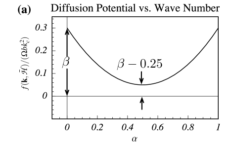
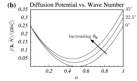
Figure 1: Dimensionless diffusion potential prefactors vs. dimensionless wave number. (a) The one dimensional or isotropic case with $\beta=0.3$. (b) The elastically isotropic case with anisotropy $\epsilon_{A}=0.1$ (see Eq. (22)).

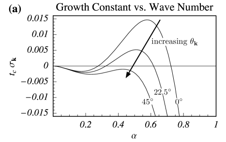
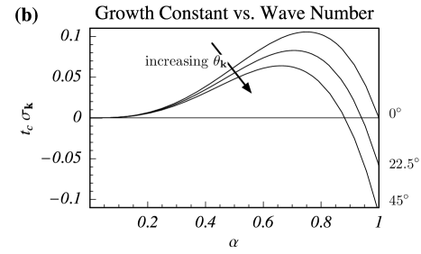
Figure 2: Dimensionless growth constant vs. dimensionless wave number. Curves are plotted for the elastically anisotropic case, but the curves marked $0^{\circ}$ are the same as for the isotropic cases. In (a), $\beta=0$. In (b) $\beta=0.2$.

Fig. 1a shows $f(\mathbf{k},\bar{0pt})/\Omega bk_{c}^{2}$ vs. $\alpha$ for an isotropic or one dimensional surface. Figs. 2 shows $t_{c}\sigma_{\mathbf{k}}$ vs. $\alpha$ for a 2D anisotropic surface (Sec. 2.2). However, the curves marked $0^{\circ}$ are identical to the dispersion relation for a 1D or 2D isotropic surface (compare Eqs. (9) and (23)).

2.1.3 Peaks

The peak growth rate and the corresponding wavenumber $k$ can be found from Eq. (16). $\sigma_{\mathbf{k}}$ has a peak at $k_{0}=k_{c}\alpha_{0}$ where

$$\alpha_{0}=\frac{1}{8}\left(3+\sqrt{9-32\beta}\right).$$ (17)

Expanding $\sigma_{\mathbf{k}}$ about this peak to second order in $k-k_{0}$,

$$\sigma_{\mathbf{k}}\approx\sigma_{0}-\frac{1}{2}\sigma_{2}(k-k_{0})^{2}$$

The two constants are

$$\sigma_{0}=\frac{1}{4}t_{c}^{-1}\alpha_{0}^{2}\left(\alpha_{0}-2\beta\right),$$ (18)

and

$$\sigma_{2}=t_{c}^{-1}k_{c}^{-2}\left(3\alpha_{0}-4\beta\right).$$ (19)

Inserting this approximation for $\sigma_{\mathbf{k}}$ into Eq. (13),

$$h_{\mathbf{k}}(t)=h_{\mathbf{k}}(0)e^{\sigma_{0}t}e^{-\frac{1}{2}\sigma_{2}t(k-k_{0})^{2}}.$$ (20)

The individual initial surface fluctuation components grow with a gaussian shaped envelope. An example of this envelope is plotted in Fig. 3(a).

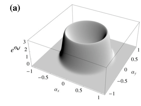
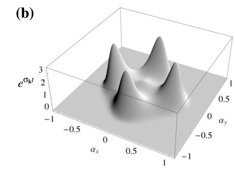
Figure 3: Exponential Envelope $e^{\sigma_{\mathbf{k}}t}$ as function of $\boldsymbol{\alpha}$ for $\beta=0.208$ and $t/t_{c}=100$. (a) 2D isotropic surface. (b) 2D anisotropic surface with $\epsilon=0.1236$.

Notice that in two dimensions, the envelope forms a ring as the peak is about the wave-number $k_{0}$ but not about any particular point in the $\mathbf{k}$-plane.

2.1.4 Stability and wetting potential

Stranski-Krastanow growth is marked by a transition from stable two-dimensional growth to unstable three-dimensional growth once a critical height $0pt_{c}$ is reached. [1] Eqs. (17), (18) and (20) are useful for analyzing the transition from stable to unstable growth. In order for this transition to occur, there must be some stabilizing term in the diffusion potential. In the present model, this means that there must be some surface energy-like term that varies strongly with film height. This condition equates to stating that $W^{\prime\prime}(\bar{0pt})$ or $F_{sw}^{20}$ or $c$ (Eq. (9)) must be rather large if $\bar{0pt}<0pt_{c}$. However, as $\bar{0pt}$ increases, these terms are reduced. Finally, when $\bar{0pt}>0pt_{c}$, this term is no longer capable of stabilizing the film against fluctuations of all possible wavelengths.

The critical value $0pt_{c}$ can be found using the analysis from [33]. By inspection of Eqs. (8), (9) and (12), modes with $f>0$ increase the total free energy $\mathcal{F}$ as they grow; thus, they are stable and decay with time. Modes with $f<0$ decrease the total free energy $\mathcal{F}$ as they grow; thus, they are unstable and grow with time. This growth and decay rule is easily verified by inspection of Eq. (14). Thus, stable growth occurs when $f(\mathbf{k},\bar{0pt})>0$ for all values of $\mathbf{k}$, and unstable growth occurs when $f(\mathbf{k},\bar{0pt})<0$ for some values of $\mathbf{k}$. Thus, the transition from stable to unstable growth occurs when the minimum value of $f(\mathbf{k},\bar{0pt})$ just becomes negative. Using the same dimensional analysis as in the previous section and following the discussion of [33], one finds that the minimum value, $f_{\text{min}}=\Omega bk_{c}^{2}\left(\beta-1/4\right)$, occurs at $k_{\min}/k_{c}=\alpha_{\text{min}}=1/2$. $f_{\text{min}}$ first becomes negative, and the transition to unstable growth occurs when the dimensionless wetting parameter (Table 1) drops to a critical value, $\beta=1/4$ . $\beta>1/4$ stable 2D growth, and $\beta<1/4$ unstable 3D growth. It is reasonable to suppose that $W(\bar{0pt})$, $W^{\prime\prime}(\bar{0pt})$, and thus $\beta$ are positive monotonically decreasing functions of $\bar{0pt}$ so that the interface becomes less important for large values of $\bar{0pt}$. For example, in [50] it is assumed that $W(0pt)=B/0pt$, where $B$ is constant. When $\beta\rightarrow 0$, corresponding to large $\bar{0pt}$, the case discussed in [28] is obtained. A similar analysis can be done for cases b and c once one specifies how the terms $F_{sw}^{(20)}$ and $F_{sw}^{(02)}$ or $a$, $b$ and $c$ depend on $\bar{0pt}$.

Using a guessed form for a wetting potential, one can find the critical film height $0pt_{c}$ by setting $\beta=1/4$ . Applying this condition to case a in Eq. (3)

$$W^{\prime\prime}(0pt_{c})=\gamma k_{c}^{2}/4.$$

Using the wetting potential of  [50] as an example, $W(0pt)=B/0pt$,

$$0pt_{c}=\sqrt[3]{8B/(\gamma k_{c}^{2})}=\sqrt[3]{8B\gamma/(2M(1+\nu)\epsilon_{m}^{2})^{2}}.$$ (21)

Conversely, one can fit a wetting potential to an observed or reasonable critical layer thickness from the same condition. Using the example wetting potential from [50],

$$B=\frac{(2M(1+\nu)\epsilon_{m}^{2})^{2}0pt_{c}^{3}}{8\gamma},$$

as stated in [50].

2.2 2D Anisotropic case

Crystal anisotropy leads to a dispersion relation $\sigma_{\mathbf{k}}$ that is both quantitatively and qualitatively different from the isotropic case. Here the effect of elastic anisotropy is discussed in most detail. Other sources of anisotropy are the surface and wetting energies. For example, in [38] the surface energy density is orientation dependent which introduces a possible anisotropy in the dispersion relation. Possible sources of anisotropy are an anisotropic elastic stiffness tensor, an orientation dependent surface energy or wetting potential or anisotropic diffusion. As discussed below, the form of anisotropy to linear order in the height fluctuation, $h$, is somewhat restricted. Results are presented for 4-fold symmetric surfaces, that is surfaces that have invariant dynamic evolution laws when rotated by $90^{\circ}$. Possible complications arising from 2-fold symmetric anisotropic terms (with $180^{\circ}$ rotational symmetry) are also discussed. As for the isotropic case, first the energetics are discussed, then the dynamics, and finally the expansion about the peaks in the dispersion relation, $\sigma_{\mathbf{k}}$.

2.2.1 Energetics

The discussion of energetics will first treat the effects of elastic anisotropy and then anisotropy resulting from surface or wetting like terms.

2.2.1.1 Elastic anisotropy

One would like to obtain a simple symbolic expression for the elastic energy density at the free surface, $\omega_{\mathbf{k}}$, to first order in $h_{\mathbf{k}}$ for the elastically anisotropic case. Similar discussions can be found in [25, 26]. For the isotropic case, $\omega_{\mathbf{k}}=-2M(1+\nu)\epsilon_{m}^{2}h_{\mathbf{k}}$. For the anisotropic case,

$$\omega_{\mathbf{k}}=-\mathcal{E}_{\theta_{\mathbf{k}}}kh_{\mathbf{k}}$$

where the prefactor $\mathcal{E}_{\theta_{\mathbf{k}}}$ is the decrease in elastic energy at the surface per unit wave number ($k\rightarrow 1$) and unit amplitude ($h_{\mathbf{k}}\rightarrow 1$) . It is not constant, but instead depends on the $\theta_{\mathbf{k}}$, the angle that $\mathbf{k}$ makes with the $x-$direction. The case of a cube-symmetry elastic stiffness tensor such as for Si is considered where one must specify three elastic constants $c_{11}$, $c_{12}$ and $c_{44}$. [51]. Growth on a (100) surface will produce an elastic energy prefactor $\mathcal{E}_{\theta_{\mathbf{k}}}$ that is four-fold symmetric (symmetric upon rotations by $90^{\circ}$). A procedure similar to [25, 26] based on a first order perturbation analysis is followed (Appendix C). A relatively simple interpolation formula [24] is hypothesized and then verified numerically.

Figure 4: Plot of $\mathcal{E}_{\theta_{\mathbf{k}}}/(M\epsilon_{m}^{2})$ for various materials. Symbols indicate values calculated using Appendix C. Solid lines are the interpolation (Eq. (22)) using the values from Table 2.

Table 2: Elastic constants [51] and calculated values (see Appendix C) for various materials of interest at $T=300\mbox{K}$.

	$c_{11}$	$c_{12}$	$c_{44}$	$M$	$\frac{\mathcal{E}_{0^{\circ}}}{M\epsilon_{0}^{2}}$	$\frac{\mathcal{E}_{45^{\circ}}}{M\epsilon_{0}^{2}}$	$\epsilon_{A}$
	$10^{11}\frac{\text{erg}}{\text{cm}^{3}}$	$10^{11}\frac{\text{erg}}{\text{cm}^{3}}$	$10^{11}\frac{\text{erg}}{\text{cm}^{3}}$	$10^{11}\frac{\text{erg}}{\text{cm}^{3}}$
Ge	12.60	4.40	6.77	13.93	2.16	1.906	0.1176
Si	16.60	6.40	7.96	18.07	2.22	1.997	0.1005
InAs	8.34	4.54	3.95	7.94	2.70	2.09	0.226
GaAs	11.90	5.34	5.96	12.45	2.15	1.87	0.1302

The interpolation procedure, suggested in [24] uses the lowest possible order expansion in $\sin(\theta_{\mathbf{k}})$ and $\cos(\theta_{\mathbf{k}})$ that has the appropriate four-fold symmetry and then interpolates between $\theta_{\mathbf{k}}=0^{\circ}$ and $\theta_{\mathbf{k}}=45^{\circ}$. Thus,

$$\mathcal{E}_{\theta_{\mathbf{k}}}=\mathcal{E}_{0^{\circ}}\left(1-\epsilon_{A}\sin^{2}\left(2\theta_{\mathbf{k}}\right)\right)$$ (22)

where $\epsilon_{A}=(\mathcal{E}_{0^{\circ}}-\mathcal{E}_{45^{\circ}})/\mathcal{E}_{0^{\circ}}$ is an anisotropy factor. This lowest order form turns out to be a very good fit to numerical calculations (Fig. 4). Table 2 gives values of $\mathcal{E}_{0^{\circ}}$ and $\epsilon_{A}$ for some systems of interest. In the elastically isotropic case, $\mathcal{E}_{0^{\circ}}=\mathcal{E}_{45^{\circ}}=2M(1+\nu)$ so that $\epsilon_{A}=0$.

There are two important differences from the elastically isotropic case. The first is obvious, that $\mathcal{E}_{\theta_{\mathbf{k}}}$ depends on angular orientation, $\theta_{\mathbf{k}}$. The second is that the peak value of $\omega_{\mathbf{k}}$ is not the same as that for the elastically isotropic case because in general, $\mathcal{E}_{0^{\circ}}\neq 2M(1+\nu)$. In [24], where the purpose was simply to investigate the mechanism by which elastic anisotropy effects order, this second difference was neglected.

2.2.1.2 Surface and Wetting Energy Anisotropy

The surface energy and wetting potential can be additional sources of anisotropy if they depend on the surface orientation so that $\gamma\rightarrow\gamma(\boldsymbol{\nabla}0pt)$ or $W(0pt)\rightarrow W(0pt,\boldsymbol{\nabla}0pt)$ (for example, [52, 38]). Then, to first order in $h$ ,

$$\mu_{\text{surf.},\mathbf{k}}=\Omega\left(\gamma k^{2}+\mathbf{k}\cdot\tilde{\boldsymbol{\gamma}}^{\prime\prime}\cdot\mathbf{k}\right)h_{\mathbf{k}}$$

where $\tilde{\boldsymbol{\gamma}}^{\prime\prime}$ is the ($2\times 2$) matrix or Hessian matrix that results from taking the second derivatives of $\gamma(\boldsymbol{\nabla}0pt)$ with respect to the two components of $\boldsymbol{\nabla}0pt$ (Appendix B.1). Similarly

$$\mu_{\text{wet},\mathbf{k}}=\Omega\left(W^{(20)}+\mathbf{k}\cdot\tilde{\mathbf{W}}^{(02)}\cdot\mathbf{k}\right)h_{\mathbf{k}}$$

where $W^{(20)}$ and $\tilde{\mathbf{W}}^{(02)}$ are the second derivatives of $W(0pt,\boldsymbol{\nabla}0pt)$ with respect to $0pt$ and $\boldsymbol{\nabla}0pt$ (Appendix B.1). For both $\mu_{\text{surf.},\mathbf{k}}$ and $\mu_{\text{wet},\mathbf{k}}$, the first term is isotropic, and the second term contains any possible anisotropy.

The rank of the $\tilde{\boldsymbol{\gamma}}^{\prime\prime}$ and $\tilde{\mathbf{W}}^{(02)}$ matrices greatly restricts the possible forms of the additional anisotropy. These $(2\times 2)$ matrices must be either two-fold symmetric or perfectly isotropic. Thus, if the surface energy and wetting potential are four-fold symmetric as $\mathcal{E}_{\theta_{\mathbf{k}}}$ is, then $\tilde{\boldsymbol{\gamma}}^{\prime\prime}\rightarrow\gamma^{\prime\prime}$, a scalar, and $\tilde{\mathbf{W}}^{(02)}\rightarrow W^{(02)}$, a scalar, and neither one contributes any additional anisotropy. They do, however, help to stabilize or further destabilize the 2D surface as they add terms proportional to $k^{2}$. The effect of these additional terms is indistinguishable from the effect of varying the value of the surface energy density, $\gamma$. [52, 31]

It should be noted that the (100) surface of a diamond or zinc-blend structures allows for anisotropy that is only 2-fold symmetric (rotations by $180^{\circ}$). Thus, they could “break” the four-fold symmetry that occurs when one considers the elastic anisotropy alone. However, this “broken” symmetry is somewhat dubious because even the diamond and zinc-blend structures have a screw symmetry (rotations by $90^{\circ}$ and translation in the [100] direction by half a lattice vector). Thus, if for example, $W(0pt,\boldsymbol{\nabla}0pt)$ is anisotropic with two-fold symmetry to linear order, there must be a fast oscillation with changes in the film height $0pt$. In Appendix D, a similar term related to anisotropic diffusion is discussed. There does not appear to be any evidence for this two-fold symmetry in the case of (100) surfaces of IV/IV systems such as Ge/Si, but in III-V/III-V systems the four-fold symmetry of the (100) surface may indeed be “broken” in this way corresponding to either a surface energy anisotropy or a diffusional anisotropy. [53, 54]. Further analysis of such terms in any more detail would greatly complicate the present discussion, so it is left for future work. Most of the modeling literature avoids this complication by not including the symmetry-breaking of the zinc-blend surface, for example [25, 26, 38].

One can perform a similar analysis of the combined surface and wetting potential, $F_{sw}(0pt,\boldsymbol{\nabla}0pt)$ (case b). To linear order the resulting anisotropic diffusion potential is (Appendix B.2)

$$\mu_{sw,\mathbf{k}}=\Omega\left(F_{sw}^{(20)}+\mathbf{k}\cdot\tilde{\mathbf{F}}_{sw}^{(02)}\cdot\mathbf{k}\right)h_{\mathbf{k}}.$$

Again, $\tilde{\mathbf{F}}_{sw}^{(02)}$ is a rank 2 tensor, and all of the same symmetry considerations apply here as well.

Because the two-fold symmetry anisotropic terms are excluded from the current discussion, and isotropic terms simply “renormalize” the effective of surface energy, there will be no further consideration of anisotropy resulting from the surface energy or wetting potential in this discussion. Further calculations will proceed assuming that the surface energy density, $\gamma$, nor the wetting potential, $W(0pt)$, depend on $\boldsymbol{\nabla}0pt$ or similarly that $F_{sw}(0pt,\boldsymbol{\nabla}0pt)$ has a purely isotropic dependence on $\boldsymbol{\nabla}0pt$. This assumption can be made without affecting any of the qualitative results.

2.2.1.3 total diffusion potential

Having dispensed with the discussion of the various sources of anisotropy, the total diffusion potential is stated for the case of 4-fold symmetric elastic anisotropy and a completely isotropic surface energy and wetting potential. $\mu_{\mathbf{k}}=f(\mathbf{k},\bar{0pt})$ with

$$f(\mathbf{k},\bar{0pt})=\begin{cases}\Omega\left[-\mathcal{E}_{0^{\circ}}\left(1-\epsilon_{A}\sin^{2}(2\theta_{\mathbf{k}})\right)k+\gamma k^{2}+W^{\prime\prime}(\bar{0pt})\right]&;\text{ case a (Eq.\,\eqref{eq:mu1})}\\ \Omega\left[-\mathcal{E}_{0^{\circ}}\left(1-\epsilon_{A}\sin^{2}(2\theta_{\mathbf{k}})\right)k+F_{sw}^{(02)}k^{2}+F_{sw}^{(20)}\right]&;\text{ case b (Eq.\,\eqref{eq:mu2}})\\ -a\left(1-\epsilon_{A}\sin^{2}(2\theta_{\mathbf{k}})\right)+bk^{2}+c&;\text{ case c (general)}\end{cases}.$$ (23)

2.2.2 Dynamics

Table 3: Characteristic wave-numbers, characteristic times and associated dimensionless variables for the three cases addressed in Eq. (9)

	$k_{c}$	$t_{c}$	$\boldsymbol{\alpha}$	$\beta$
case a	$\mathcal{E}_{0^{\circ}}/\gamma$	$\gamma^{3}/(\mathcal{D}\Omega\mathcal{E}_{0^{\circ}}^{4})$	$\mathbf{k}/k_{c}$	$\gamma W^{\prime\prime}(\bar{0pt})/\mathcal{E}_{0^{\circ}}^{2}$
case b	$\mathcal{E}_{0^{\circ}}/F_{sw}^{(02)}$	$\left(F_{sw}^{(02)}\right)^{3}/(\mathcal{D}\Omega\mathcal{E}_{0^{\circ}}^{4})$	$\mathbf{k}/k_{c}$	$F_{sw}^{(02)}F_{sw}^{(20)}/\mathcal{E}_{0^{\circ}}^{2}$
case c	$a/b$	$b^{3}/(\mathcal{D}\Omega a^{4})$	$\mathbf{k}/k_{c}$	$cb/a^{2}$

The dynamics is governed by surface diffusion, just as for the fully isotropic case. It is assumed that the diffusivity is isotropic as was done for the surface energy and the wetting energies; thus, all anisotropy in the film evolution dynamics comes from elastic effects alone. The possibility and effects of an anisotropic diffusion potential is discussed in Appendix D (also see [54]). The time dependence of the surface perturbations simply follows Eqs. (13) and (14), but with Eq. (23) used for $f(\mathbf{k},\bar{0pt})$. As for the isotropic case, appropriate characteristic wave numbers ($k_{c}$) and time scales ($t_{c}$) can be found for each of the three cases along with the associated dimensionless wave vector $\boldsymbol{\alpha}$ and dimensionless wetting parameter $\beta$. These are listed in Table 3. The dispersion relation, $\sigma_{\mathbf{k}}$ can be expressed in terms of these dimensionless variables ($\boldsymbol{\alpha}$ and $\beta$), giving

$$\sigma_{\mathbf{k}}=\sigma_{k_{c}\boldsymbol{\alpha}}=t_{c}^{-1}\alpha^{2}\left[\alpha\left(1-\epsilon_{A}\sin^{2}(2\theta_{\mathbf{k}})\right)-\alpha^{2}-\beta\right].$$ (24)

The stability behavior is essentially the same as for the isotropic case with a transition occurring at $\beta=1/4$ corresponding to $\bar{0pt}=0pt_{c}$.

2.2.3 Expansion about peaks

$\sigma_{\mathbf{k}}$ has $4$ peaks at $(\mathbf{k},\theta_{\mathbf{k}})=(k_{0},\pi[n-1]/2)$ with $k_{0}=k_{c}\alpha_{0}$ (Eq. (17)) and $n=1\dots 4$. In vector form, there are four peaks at

$$\mathbf{k}_{n}=k_{0}\left(\cos(\pi(n-1)/2)\mathbf{i}+\sin(\pi(n-1)/2)\mathbf{j}\right).$$

Similar to the isotropic case, $\sigma_{\mathbf{k}}$ can be expanded about individual peaks so that in the vicinity of peak $n$, $\sigma_{\mathbf{k}}\approx\sigma_{n}$ with

$$\sigma_{n}=\sigma_{0}-\frac{1}{2}\sigma_{\parallel}(k-k_{0})^{2}-\frac{1}{2}\sigma_{\perp}k_{0}^{2}(\theta_{\mathbf{k}}-n\pi/2)^{2},$$

where $\sigma_{0}$ is given by Eq. (18), $\sigma_{\parallel}=\sigma_{2}$ given by Eq. (19), and

$$\sigma_{\perp}=8\epsilon_{A}\alpha_{0}t_{c}^{-1}k_{c}^{-2}.$$

In terms of the vector components parallel and perpendicular to $\mathbf{k}_{n}$, $k_{\parallel}$ and $k_{\perp}$ respectively,

$$\sigma_{n}=\sigma_{0}-\frac{1}{2}\sigma_{\parallel}(k_{\parallel}-k_{0})^{2}-\frac{1}{2}\sigma_{\perp}k_{\perp}^{2},$$

$k_{\parallel}=\cos[\pi(n-1)/2]k_{x}+\sin[\pi(n-1)/2]k_{y}$, and $k_{\perp}=-\sin[\pi(n-1)/2]k_{x}+\cos[\pi(n-1)/2]k_{y}$ . The time evolution of $h_{\mathbf{k}}$in the vicinity of one of the $\mathbf{k}_{n}$ is

$$h_{\mathbf{k}}(t)\approx h_{\mathbf{k}}(0)e^{t\left(\sigma_{0}-\frac{1}{2}\sigma_{2}(k_{\parallel}-k_{0})^{2}-\frac{1}{2}\sigma_{\perp}k_{\perp}^{2}\right)}.$$

3 Correlation Functions

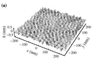
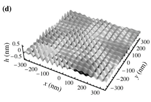
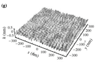
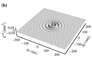
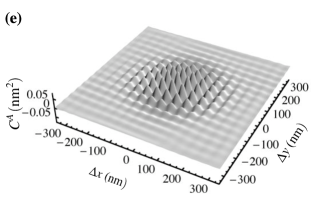
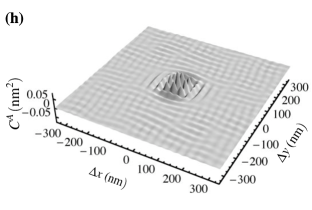
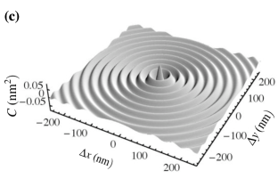
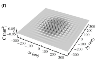
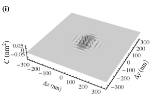
Figure 5: Film heights and real-space correlation functions for Ge/Si as discussed in Sec. 4. All units are in nm or $\text{nm}^{2}$. (a-c) show respectively example $h(\mathbf{x})$ , corresponding $C^{A}(\boldsymbol{\Delta}\mathbf{x})$ and calculated $C(\boldsymbol{\Delta}\mathbf{x})$ for the 2D isotropic surface with $\beta=0.208$ and $t/t_{c}=306$. Fig. c uses Eq. (48) because the corresponding formula for $C(\boldsymbol{\Delta}\mathbf{x})$ with finite $L_{\text{cor}}$ is not available. (d-f) show the same for the 2D anisotropic surface with $\beta=0.208$ and $t/t_{c}=430$. Eq. (50) is used for plot (f). (g-i) show the same for $\beta=0$ and $t/t_{c}=40.3$. Eq. (50) is used for plot (i).

Correlation functions and associated constants such as correlation lengths can be very useful for characterizing order. In particular, the autocorrelation function (Eq. (25)) and its Fourier transform (Eq. (26)) also known as the spectrum function can give a very good characterization of dot order (Figs. 6a and c and 5b, e and h). The autocorrelation function is denoted $C^{A}(\boldsymbol{\Delta}\mathbf{x})$ where $\boldsymbol{\Delta}\mathbf{x}$ is the difference vector between two points in the $\mathbf{x}-$plane. The spectrum function is a function of $\mathbf{k}$, and it is denoted $C_{\mathbf{k}}^{A}$. The goal here is to be able to predict these two functions and to describe them quantitatively in a manner that can be used to characterize SAQD order with just a few numbers. The autocorrelation function is the result of a spatial average over one experiment or one simulation (numerical experiment). It is regular and repeatable because it is closely tied to the correlation function and spectrum function that results from an ensemble average (Eqs. X and X). These are denoted as $C(\boldsymbol{\Delta}\mathbf{x})$ and the spectrum $C_{\mathbf{k}}$ respectively. Note that the ensemble averaged functions do not have a superscript “$A$.” These ensemble average correlation functions are useful in the analysis of stochastic ordinary and partial differential equations. [55, 56]. From a strictly technical viewpoint, the spatial average and the ensemble average are not exactly the same; however, they are closely enough connected that it is reasonable to use one as a substitute for the other (Sec. 3.1 and Appendix 3).

In the following, the analysis of SAQD order via autocorrelation and correlation functions is discussed (Sec. 3.1). Then, the stochastic initial conditions are discussed (Sec. 3.2). Then, the prediction of the Fourier transforms of the correlation functions is discussed (Sec. 3.3). The real-space correlation functions are presented (Sec. 3.4). Finally, there are some notes regarding generalizing the analysis method to any dispersion relation that has peaks (Sec. 3.5), for example, peaks related to broken four-fold symmetry or growth on a miscut substrate.

3.1 Correlation Functions and SAQD order

Auto-correlation functions are well-suited for investigating SAQD order. The autocorrelation function is defined as

$$C^{A}(\boldsymbol{\Delta}\mathbf{x})=\frac{1}{A}\int d^{2}\mathbf{x}^{\prime}\,h(\boldsymbol{\Delta}\mathbf{x}+\mathbf{x^{\prime}})h(\mathbf{x}^{\prime})^{*}.$$ (25)

Its Fourier transform sometimes called the spectrum [56], spectrum function or power spectrum is

$$C_{\mathbf{k}}^{A}=\frac{1}{(2\pi)^{d}}\int d^{2}\boldsymbol{\Delta}\mathbf{x}\,e^{-i\mathbf{k}\cdot\boldsymbol{\Delta}\mathbf{x}}C(\boldsymbol{\Delta}\mathbf{x})=\frac{(2\pi)^{d}}{A}\left|h_{\mathbf{k}}\right|^{2},$$ (26)

where $A$ is the projected area of the film in the $x-y-$plane. A periodic array of SAQDs leads to a periodic auto-correlation function. A nearly periodic array leads to a range-limited periodic auto-correlation function. The ensemble-mean of these autocorrelation functions can be calculated, and it is a good predictor of a SAQD order.

3.1.1 Periodic array

Consider a perfectly periodic height fluctuation corresponding to a perfect lattice of SAQDs,

$$h(\mathbf{x})=\frac{h_{0}}{N}\sum_{i=n}^{N}\exp\left[i\mathbf{k}_{n}\cdot\left(\mathbf{x}-\mathbf{x}_{O}\right)\right]$$ (27)

plus higher order harmonic, where the dots have a height proportional to $h_{0}$, $N$ is the degree of symmetry, probably, 4-fold or 6-fold, $\mathbf{x}_{O}$ is a random origin offset.

$$\mathbf{k}_{n}=k_{0}\left(\cos\left(\frac{2\pi(n-1)}{N}\right)\mathbf{i}+\sin\left(\frac{2\pi(n-1)}{N}\right)\mathbf{j}\right),$$

In a linear analysis, the higher order harmonics do not come into play, so they are neglected here. In reciprocal space,

$$h_{\mathbf{k}}=\frac{h_{0}}{N}\sum_{n=1}^{N}e^{-i\mathbf{k}_{n}\cdot\mathbf{x}_{O}}\delta^{d}(\mathbf{k}-\mathbf{k}_{n})$$

plus higher order harmonic. The autocorrelation function is found by plugging Eq. (27) into Eq. (25) and simplifying,

$$C^{A}(\boldsymbol{\Delta}\mathbf{x})=\left(\frac{h_{0}}{N}\right)^{2}\sum_{n=1}^{N}\exp\left[i\mathbf{k}_{n}\cdot\boldsymbol{\Delta}\mathbf{x}\right]$$ (28)

plus higher order harmonic. In finding Eq. (28), the relation

$$\int d^{2}\mathbf{x}^{\prime}\,e^{i\left(\mathbf{k}_{m}-\mathbf{k}_{n}\right)\cdot\mathbf{x}^{\prime}}=A\delta_{\mathbf{k}_{m}\mathbf{k}_{n}}=(2\pi)^{d}\delta^{d}(\mathbf{k}_{m}-\mathbf{k}_{n})$$ (29)

has been used. $\delta_{\mathbf{k}\mathbf{k}^{\prime}}$ is the Kronecker Delta, and $\delta^{d}(\mathbf{k}-\mathbf{k}^{\prime})$ is the Dirac Delta. Eq. (29) will be helpful whenever it is necessary to take an areal average or sum over Dirac Delta functions. In reciprocal space,

$$C_{\mathbf{k}}^{A} = \frac{(2\pi)^{2}}{A}\frac{h_{0}^{2}}{N^{2}}\sum_{m,n=1}^{N}\delta^{2}(\mathbf{k}-\mathbf{k}_{m})\delta^{2}(\mathbf{k}-\mathbf{k}_{n})$$ (30)

$$= \frac{h_{0}^{2}}{N^{2}}\sum_{i=1}^{N}\delta^{2}(\mathbf{k}-\mathbf{k}_{i})$$

plus higher order harmonics, where $\delta^{d}(\mathbf{k}-\mathbf{k}_{n})=(A/(2\pi)^{d})\delta_{\mathbf{k}\mathbf{k}_{n}}$.. Thus, the order of the SAQD lattice manifests itself as periodic functions in real-space (Eq. (28)) and sharp peaks in reciprocal space (Eq. (30)).

3.1.2 Nearly Periodic array

A nearly periodic arrays shows deviation from perfect order. This deviation is shows itself by broadening of the peaks of the spectrum function, $C_{\mathbf{k}}^{A}$, and by range limited periodicity of the real-space autocorrelation function, $C^{A}(\boldsymbol{\Delta}\mathbf{x})$. These two measure of disorder are naturally related.

The disorder in lateral dot size $\Delta_{\text{size}}$ and spacing, $\Delta_{\text{spacing}}$ are related to each other and to the broadening of the peaks in $C_{\mathbf{k}}^{A}$ (Fig. 6.a and c). Prior to ripening, the size and spatial order should be related, as the volume of a dot should be proportional to the amount of nearby material. If the SAQDs have nearly uniform size and spacing (peak-to-peak distance) $L_{0}$, the reciprocal space autocorrelation function will be tightly clustered around the wavenumber characterizing the dot spacing $k_{0}=2\pi/L_{0}$. There are a number of such peaks depending on the system symmetry (Fig. 6.a and c), but consider just one. Since the order is not perfect, the peak will have a finite width. Consequently, there will be a scatter in the dot size. Since $L_{\text{0}}=2\pi/k_{0}$, the scatter in dot spacing ($\Delta_{\text{spacing}}$) is related to the scatter in Fourier components ($\Delta_{k}$). Taking the derivative of the spacing-wavenumber relation and rearranging,

$$\frac{\Delta_{\text{spacing}}}{L_{0}}\approx\frac{\Delta_{k}}{k_{0}}.$$

It is reasonable to expect that the fractional disorder in size ($\Delta_{\text{size }}/L_{\text{size}}$) is given by a similar (if not exactly the same) number.

Another way to view spatial order (periodicity) is not by dot-dot distances, but the distance over which the dot array can be considered periodic. This limited periodicity is evident in the film height autocorrelation function (Eq. (25) and Figs. 5.b, e and h). Consider two distant dots. Their position will be completely uncorrelated, so it will be completely random as to whether one position corresponds to a peak or a valley. Thus, for a large differences in position the autocorrelation function tends to zero.

$$C^{A}(\boldsymbol{\Delta}\mathbf{x}_{\text{large}})=0$$

Similarly, the mean-square fluctuation of the film height can be large so that

$$C^{A}(\boldsymbol{\Delta}\mathbf{x}=0)\gg 0.$$

The distance over which the autocorrelation function, $C^{A}(\boldsymbol{\Delta}\mathbf{x})$ decays to $0$ is the correlation length, $L_{\text{cor}}$. Thus, $L_{\text{cor}}$ is a reasonable measure of spatial order.

The two measures of order $\Delta_{\text{spacing}}$ and $L_{\text{cor}}$ are intrinsically linked. The well known rule of Fourier transforms states that the product of the real-space and reciprocal space widths must be greater than or equal to unity. Thus, $\Delta_{k}L_{\text{cor}}\geq 1$, or $\Delta_{\text{spacing}}\geq 2\pi L_{0}^{2}/L_{\text{cor}}$. Similarly, one can expect that $\Delta_{\text{size}}\sim L_{\text{size}}^{2}/L_{\text{cor}}$. Thus, assuming that dot size is governed by the amount of nearby material, small dispersions in dot size are only possible if there is long correlation length.

3.1.3 Ensemble Correlation Functions / ergodicity

SAQDs are seeded by random fluctuations. Consequently, each experiment or simulation must be treated as just one possible realization, and the autocorrelation function will be different for each realization. Thus, for analytic predictions, one must rely on ensemble averages. In [24], it was assumed that the ensemble average correlation function was a good description of a SAQD order, an assumption that was born out by numerical calculations. Now, this relation is put on a more solid ground. In particular, it is found that the ensemble correlation functions provide good estimates of the auto correlation function and spectrum function produced by any particular realization. First, it is shown that the mean value of the film-height fluctuation is zero. Then the method to calculate the ensemble-averaged autocorrelation function and spectrum function is presented. Additional mathematical details are presented in Appendix 3.

3.1.3.1 Mean fluctuation

It is fairly straightforward to show that the ensemble mean film-height fluctuation is zero. The governing dynamics (Eq. (12)) is invariant upon the substitution $h(\mathbf{x},t)\rightarrow-h(\mathbf{x},t)$. Thus, assuming that one does not bias the initial conditions the mean fluctuations must be zero for all time,

$$\left\langle h(\mathbf{x},t)\right\rangle=\left\langle-h(\mathbf{x},t)\right\rangle=0\text{, and }\left\langle h_{k}(t)\right\rangle=0.$$

This is a common situation, and it is most appropriate to characterize the film height fluctuations using the two-point correlation function (or simply “the correlation function”). [55]

3.1.3.2 Correlation Function

The autocorrelation function can be estimated by its ensemble average. Furthermore, this ensemble average is equivalent to the correlation function that can be easily calculated analytically. These relations are first discussed for the real-space correlation functions and then their Fourier transforms. First, the statistical properties of the autocorrelation function are discussed. Then the statistical properties of the spectrum function. Finally, the method to The main results are reported here, and details of derivations are reported in Appendix E.

First it is noted that the autocorrelation function averaged over all realizations is equal to the ensemble correlation function.

$$\left\langle C^{A}(\boldsymbol{\Delta}\mathbf{x})\right\rangle=C(\boldsymbol{\Delta}\mathbf{x})\text{, where }C(\boldsymbol{\Delta}\mathbf{x})=\left\langle h(\boldsymbol{\Delta}\mathbf{x})h(\mathbf{0})\right\rangle,$$ (31)

where $\left\langle\dots\right\rangle$ indicate an ensemble average. Eq. (31) assumes that the model of film-growth is translationally invariant. This relationship is fortunate, in that it allows one to predict the “typical” autocorrelation function using analytic tools that apply only to ensemble averages.

Second, it is noted that as the area that is used to calculate the autocorrelation function becomes large, the autocorrelation function tends towards it mean value,

$$C^{A}(\boldsymbol{\Delta}\mathbf{x})\approx C(\boldsymbol{\Delta}\mathbf{x})+O[A^{-1/2}],$$ (32)

where $O[A^{-1/2}]$ indicates statistical fluctuations about the mean value that become smaller and smaller as the area in an experiment or the simulation area in a numerical experiment becomes larger. These fluctuations or noise die out as $A^{1/2}$. For example, the autocorrelation functions in Figs. 5.e and h are very close to the ensemble average autocorrelation functions Figs. 5.f and h, but have random fluctuations that are most visible far from the origin. This property, that averaging over a parameter such as position is equivalent to averaging over all realizations, is known as ergodicity. Individual realizations are tightly distributed about a “typical” behavior. This tight distribution lends credibility to the notion that one can have representative experiments or simulations. Unfortunately, the “demonstration” of Eq. (32) in Appendix E is not as general as one might like. Rigorously, it applies when the Fourier components of film height ($h_{\mathbf{k}}$) are independent and normally distributed; however, it is reasonable to conjecture that a relationship like Eq. (32) holds whenever the statistical distribution of film heights is suitably bounded as the boundedness of $C_{\mathbf{k}}^{A}$ plays an important role in the derivations.

In reciprocal space, one finds that the ensemble-mean spectrum function is

$$\left\langle C_{\mathbf{k}}^{A}\right\rangle=C_{\mathbf{k}},$$ (33)

where $C_{\mathbf{k}}$ is defined as the prefactor appearing in the reciprocal-space two-point correlation function.

$$C_{\mathbf{k}\mathbf{k}}=\left\langle h_{\mathbf{k}}h_{\mathbf{k}}^{*}\right\rangle=C_{\mathbf{k}}\delta^{d}(\mathbf{k}-\mathbf{k}^{\prime})=C_{\mathbf{k}}\frac{A}{(2\pi)^{d}}\delta_{\mathbf{k}\mathbf{k}^{\prime}},$$ (34)

where Eq. (29) has been used. This form for the two-point correlation function in reciprocal space occurs if and only if the system is translationally invariant. Eq. (33) is valuable because one can solve for $C_{\mathbf{k}}$ analytically in the linear case or using various analytic approximations in the non-linear case. Unlike the autocorrelation function, the spectrum function fluctuates greatly about its mean. In fact, the fluctuations are about 100% (Appendix E.2). These large fluctuations result in the commonly observed speckle pattern for the spectrum function $C_{\mathbf{k}}^{A}$(Figs. 6.a and c). Contrast this pattern with ensemble-mean spectrum function $C_{\mathbf{k}}$ shown in Figs. 6.b and d. These speckles can be removed by a smoothing operation, and a relation similar to Eq. (32) results (Appendix E.2.2). Finally, it should be noted that just as $C_{\mathbf{k}}^{A}$ is the Fourier transform of $C^{A}(\boldsymbol{\Delta}\mathbf{x})$, $C_{\mathbf{k}}$ is the Fourier transform of $C(\boldsymbol{\Delta}\mathbf{x})$ (Appendix E.1).

3.2 Stochastic Initial Conditions

To model or simulate the formation of SAQDs, it is absolutely essential to include some sort of stochastic effect. An initially flat film $h(\mathbf{x},0)=0$ is in unstable equilibrium. Thus, to seed the formation of quantum dots, it is necessary to perturb the flat surface. The simplest method to do this is to use stochastic initial conditions with deterministic evolution. One can tenuously suppose that white noise initial conditions do not “bias” the ultimate evolution of the film. [57] Thus, the initial conditions are taken from an ensemble with zero mean,

$$\left\langle h(\mathbf{x},0)\right\rangle=0.$$ (35)

and a spatial correlation function,

$$C(\mathbf{x},\mathbf{x}^{\prime},0)=\left\langle h(\mathbf{x},0)h(\mathbf{x}^{\prime},0)^{*}\right\rangle=\Delta^{2}\delta^{d}\left(\mathbf{x}-\mathbf{x}^{\prime}\right),$$ (36)

where the brackets $\left\langle\dots\right\rangle$ indicate an ensemble average, $\Delta$ is the noise amplitude, and $\delta^{d}(x)$ is the $d-$dimensional Dirac Delta function. White noise conditions have an infinite amplitude which is not physical. Thus, a minimum modification can be made to “cut off” the infinite fluctuations.

$$C(\mathbf{x},\mathbf{x}^{\prime},0)=\frac{\Delta^{2}}{(2\pi b_{0}^{2})^{d/2}}\exp\left(-\frac{\left(\mathbf{x}-\mathbf{x}^{\prime}\right)^{2}}{2b_{0}^{2}}\right)$$ (37)

In the limit $b_{0}\rightarrow 0$, this correlation function reverts to the white noise correlation functions.

In reciprocal space,

$$C_{\mathbf{k}\mathbf{k}^{\prime}}(0) = \left\langle h_{\mathbf{k}}(0)h_{\mathbf{k}^{\prime}}^{*}(0)\right\rangle$$

$$= (2\pi)^{-2d}\int d^{d}\mathbf{x}\int d^{d}\mathbf{x}^{\prime}\,e^{\left(-i\mathbf{k}\cdot\mathbf{x}+i\mathbf{k}^{\prime}\cdot\mathbf{x}^{\prime}\right)}C(\mathbf{x},\mathbf{x}^{\prime},0)$$

$$= \frac{\Delta^{2}}{(2\pi)^{d}}e^{-\frac{1}{2}b_{0}^{2}k^{2}}\delta^{d}(\mathbf{k}-\mathbf{k}^{\prime})$$

Letting $b_{0}\rightarrow 0$, the white noise reciprocal space correlation function is obtained. Thus, the initial spectrum function is

$$C_{\mathbf{k}}(0)=\frac{\Delta^{2}}{(2\pi)^{d}}e^{-\frac{1}{2}b_{0}^{2}k^{2}}.$$

The atomic-scale has a small and short-lived influence on the final film morphology (Appendix F), but the cutoff procedure is useful for choosing a reasonable value of $\Delta^{2}$. It seems reasonable to choose $\Delta^{2}$ so that the initial r.m.s. fluctuation $\sqrt{C(\mathbf{0},0)}=\left\langle h(\mathbf{0},0)h(\mathbf{0},0)^{*}\right\rangle^{1/2}$is one monolayer ($1\text{ ML}$). Also, choosing $b_{0}=1\mbox{\text{ ML}}$ as the atomic scale cutoff is

$$\Delta^{2}=(2\pi)^{d/2}(1\text{ ML})^{2+d},$$ (38)

where the natural unit $1\mbox{\text{ ML}}$ is, of course, material dependent.

Using stochastic initial conditions, one can integrate individual initial conditions to obtain representative samples and then average over many realizations, the Monte Carlo approach, or one can calculate analytically, the statistical measures of the ensemble. The ensemble statistical measures are strongly related to the statistical measures of order for an individual realization, so the second approach is opted for here. Thus, the predicted SAQD order is ultimately stated in terms of ensemble correlation functions.

3.3 Reciprocal Space Correlation Functions

The reciprocal space correlation function, $C_{\mathbf{k}\mathbf{k}^{\prime}}$, and spectrum function, $C_{\mathbf{k}}$, are calculated for the 1D and 2D isotropic case and then for the 2D anisotropic case. Generally $C_{\mathbf{k}}$ includes the length scales introduced in Sec. 2.1.3 as well as the atomic scale cutoff $b_{0}$.

$$C_{\mathbf{k}\mathbf{k}^{\prime}} = \left\langle h_{\mathbf{k}}(t)h_{\mathbf{k}^{\prime}}^{*}(t)\right\rangle=e^{(\sigma_{\mathbf{k}}+\sigma_{\mathbf{k}^{\prime}})t}\left\langle h_{\mathbf{k}}(0)h_{\mathbf{k}^{\prime}}(0)^{*}\right\rangle$$ (39)

$$= \frac{\Delta^{2}}{(2\pi)^{2}}e^{(\sigma_{\mathbf{k}}+\sigma_{\mathbf{k}^{\prime}})t-\frac{1}{2}b_{0}^{2}k^{2}}\delta^{2}(\mathbf{k}-\mathbf{k}^{\prime}).$$

Without much error, $b_{0}$ can be neglected in the exponential (Appendix F). Using Eq. (34), the spectrum function is then identified as

$$C_{\mathbf{k}}=\frac{\Delta^{2}}{(2\pi)^{d}}e^{2\sigma_{\mathbf{k}}t}.$$ (40)

$C_{\mathbf{k}}$ is now calculated for each model: 1D isotropic, 2D isotropic and 2D anisotropic.

3.3.1 one-dimensional

The one dimensional surface is the simplest, so it is treated first. The spectrum function is simply

$$C_{\mathbf{k}}=\frac{\Delta^{2}}{2\pi}e^{2\sigma_{0}t-\frac{1}{2}(2\sigma_{2}t)(k-k_{0})^{2}}.$$

$C_{\mathbf{k}}$ has a peak at $\mathbf{k}=\pm k_{0}\mathbf{i}$. One can easily read off the correlation length as

$$L_{\text{cor}}=\sqrt{2\sigma_{2}t}=k_{c}^{-1}\sqrt{2(3\alpha_{0}-4\beta)(t/t_{c})}.$$ (41)

so that

$$C_{\mathbf{k}}=\frac{\Delta^{2}}{2\pi}e^{2\sigma_{0}t-\frac{1}{2}L_{\text{cor}}^{2}(k-k_{0})^{2}}.$$

This approximation is valid when $k_{0}L_{\text{cor}}\gg 1$. In terms of $k_{x}$,

$$C_{\mathbf{k}}=\frac{\Delta^{2}}{2\pi}e^{2\sigma_{0}t}\left(e^{-\frac{1}{2}L_{\text{cor}}^{2}(k_{x}-k_{0})^{2}}+e^{-\frac{1}{2}L_{\text{cor}}^{2}(k_{x}+k_{0})^{2}}\right)$$

3.3.2 2D isotropic

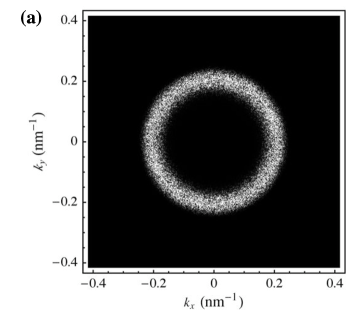
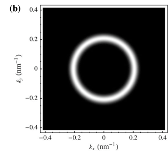
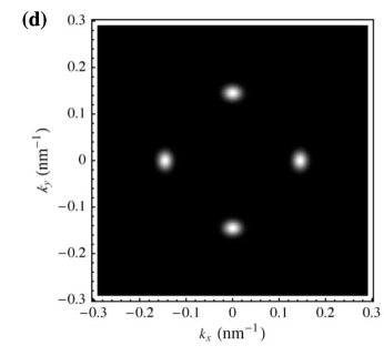
Figure 6: $C_{\mathbf{k}}^{A}$ and $C_{\mathbf{k}}$ for Ge/Si as discussed in Sec. 4. (a,b) 2D isotropic surface. Eq. (42) is used for $C_{\mathbf{k}}$. (c,d) 2D anisotropic surface. Eq. (43) is used for $C_{\mathbf{k}}$.

The 2D isotropic case is very similar;

$$C_{\mathbf{k}}=\frac{\Delta^{2}}{(2\pi)^{2}}e^{2\sigma_{0}t-\frac{1}{2}L_{\text{cor}}^{2}(k-k_{0})^{2}},$$ (42)

where $L_{\text{cor}}$ is the same as in Eq. (41). It has maximum that forms a ring in the $\mathbf{k}-$plane as graphed in Fig. 6.b.

3.3.3 anisotropic

The anisotropic spectrum function is

$$C_{\mathbf{k}} = \frac{\Delta^{2}}{(2\pi)^{2}}e^{2\sigma_{0}t}\sum_{n=1}^{4}e^{-\frac{1}{2}L_{\parallel}^{2}\left(k_{\parallel}-k_{0}\right)^{2}-\frac{1}{2}L_{\perp}^{2}k_{\perp}^{2}},$$ (43)

where

$$L_{\parallel}=\sqrt{2\sigma_{\parallel}t}=k_{c}^{-1}\sqrt{(6\alpha_{0}-8\beta)(t/t_{c})},$$ (44)

$$L_{\perp}=\sqrt{2\sigma_{\perp}t}=k_{c}^{-1}\sqrt{16\epsilon\alpha_{0}(t/t_{c})},$$ (45)

$k_{\parallel}=\cos[\pi(n-1)/2]k_{x}+\sin[\pi(n-1)/2]k_{y}$, and $k_{\perp}=-\sin[\pi(n-1)/2]k_{x}+\cos[\pi(n-1)/2]k_{y}$ and it is graphed in Fig. 6.d. This approximation is valid when $k_{0}L_{\parallel}\gg 1$ and $k_{0}L_{\perp}\gg 1$.

Loosely speaking, one can argue that the isotropic case is similar to letting $\epsilon_{A}\rightarrow 0$ in Eq. (45) so that the perpendicular correlation length is always 0 regardless of time. A more conservative approach would be to argue that $L_{\perp}\approx 2\pi/k_{0}$ for the isotropic model via inspection of Figs. 6(a) and (b). Even still, the more conservative result guarantees that the perpendicular correlation length will always be the same as the dot spacing; thus, it will always limit SAQD order to the first nearest neighbor at best.

3.4 Real Space Correlation Functions

The real space correlation functions $C(\boldsymbol{\Delta}\mathbf{x})$ are now calculated for the 1D and 2D isotropic cases and the 2D elastically anisotropic case.

3.4.1 one-dimensional

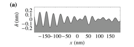
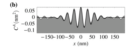
Figure 7: 1D isotropic surface in real space for Ge/Si as discussed in Sec. 4. (a) Example of $h(\mathbf{x})$ plotted over a length of $8L_{\text{cor}}$. (b) corresponding reals space correlation functions plotted for range $\pm 4L_{\text{cor}}$. Filled plot is an example of $C^{A}(\boldsymbol{\Delta}\mathbf{x})$. Solid line is$C(\boldsymbol{\Delta}\mathbf{x})$ (Eq. (46)).

In one dimension,

$$C(\boldsymbol{\Delta}\mathbf{x}) = \int_{-\infty}^{\infty}dk_{x}\,e^{ik_{x}\boldsymbol{\Delta}\mathbf{x}}C_{\mathbf{k}}$$ (46)

$$= \frac{\Delta^{2}}{\sqrt{2\pi}}\frac{1}{L_{\text{cor}}}e^{2\sigma_{0}t-\frac{1}{2}\Delta x^{2}/L_{\text{cor}}^{2}}2\cos\left(k_{0}x\right).$$

Thus, $C(\boldsymbol{\Delta}\mathbf{x})$ has a damped periodicity indicating that it is imperfectly periodic (Fig. 7).

3.4.2 2D isotropic

In two dimensions with elastic isotropy,

$$C(\boldsymbol{\Delta}\mathbf{x}) = \int d^{2}\mathbf{k}\,e^{i\mathbf{k}\cdot\boldsymbol{\Delta}\mathbf{x}}C_{\mathbf{k}}$$

$$= \frac{\Delta^{2}}{(2\pi)^{2}}e^{2\sigma_{0}t}\int_{0}^{2\pi}d\theta_{\mathbf{k}}\int_{0}^{\infty}dk\,ke^{i(k\Delta x\cos(\theta_{\mathbf{k}}-\theta_{\boldsymbol{\Delta}\mathbf{x}})}e^{-\frac{1}{2}L_{\text{cor}}^{2}(k-k_{0})^{2}}.$$

Performing the angular integration first,

$$C(\boldsymbol{\Delta}\mathbf{x})=\frac{\Delta^{2}}{2\pi}e^{2\sigma_{0}t}\int_{0}^{\infty}dk\,kJ_{0}(k\Delta x)e^{-\frac{1}{2}L_{\text{cor}}^{2}(k-k_{0})^{2}},$$

where $J_{0}$ is the zeroth Bessel function. In general, this integral is best performed numerically; however, it can be solved in two important cases: $\boldsymbol{\Delta}\mathbf{x}\rightarrow\mathbf{0}$ and $L_{\text{cor}}\rightarrow\infty$ (corresponding to long times). In the first case,

$$C(\boldsymbol{\Delta}\mathbf{x}) = \frac{\Delta^{2}}{2\pi}e^{2\sigma_{0}t}\int_{0}^{\infty}dk\,ke^{-\frac{1}{2}L_{\text{cor}}^{2}(k-k_{0})^{2}}.$$

Under the same conditions that Eq. (42) is valid ($k_{0}L_{\text{cor}}\gg 1$), the lower limit of the integral can be approximated as $-\infty$ so that

$$C(\boldsymbol{\Delta}\mathbf{x}=\mathbf{0})=\frac{\Delta^{2}k_{0}}{\sqrt{2\pi}L_{\text{cor}}}e^{2\sigma_{0}t}.$$ (47)

This function gives the mean square surface height fluctuation. In the second case where $L_{\text{cor}}\rightarrow\infty$, $e^{-\frac{1}{2}L_{\text{cor}}^{2}(k-k_{0})^{2}}\rightarrow(2\pi)^{1/2}L_{\text{cor}}^{-1}\delta(k-k_{0})$, so that

$$C(\boldsymbol{\Delta}\mathbf{x}) = \frac{\Delta^{2}k_{0}}{\sqrt{2\pi}L_{\text{cor}}}e^{2\sigma_{0}t}J_{0}\left(k_{0}\Delta x\right).$$ (48)

This correlation function is the most ordered case for a 2D isotropic surface. It is graphed in Fig. 5c.

3.4.3 anisotropic

To find the real-space correlation function for the elastically anisotropic case, it is best to find the contribution from each peak and then sum so that

$$C(\boldsymbol{\Delta}\mathbf{x})=\frac{\Delta^{2}}{(2\pi)^{2}}e^{2\sigma_{0}t}\sum_{n=1}^{4}C^{n}(\boldsymbol{\Delta}\mathbf{x})$$ (49)

where

$$C^{n}(\boldsymbol{\Delta}\mathbf{x})=\int d^{2}\mathbf{k}\,e^{i\mathbf{k}\cdot\mathbf{x}}e^{-\frac{1}{2}L_{\parallel}^{2}\left(k_{\parallel}-k_{0}\right)^{2}-\frac{1}{2}L_{\perp}^{2}k_{\perp}^{2}}.$$

$\boldsymbol{\Delta}\mathbf{x}$ can be decomposed into the directions parallel and perpendicular to $\mathbf{k}_{n}$, so that $\Delta x_{\parallel}=\cos(\pi(n-1)/2)\Delta x+\sin(\pi(n-1)/2)\Delta y$ and $\Delta x_{\perp}=-\sin(\pi(n-1)/2)\Delta x+\cos(\pi(n-1)/2)\Delta y$. Thus,

$$C^{n}(\boldsymbol{\Delta}\mathbf{x}) = \left(\int dk_{\parallel}\,e^{ik_{\parallel}\Delta x_{\parallel}-\frac{1}{2}L_{\parallel}^{2}\left(k_{\parallel}-k_{0}\right)^{2}}\right)\left(\int dk_{\perp}\,e^{ik_{\perp}\Delta x_{\perp}-\frac{1}{2}L_{\perp}^{2}k_{\perp}^{2}}\right)$$

$$= \frac{2\pi}{L_{\parallel}L_{\perp}}e^{-\frac{1}{2}\left(x_{\parallel}^{2}/L_{\parallel}^{2}+x_{\perp}^{2}/L_{\perp}^{2}\right)}e^{ik_{0}x_{\parallel}}.$$

Plugging into Eq. (49),

$$C(\boldsymbol{\Delta}\mathbf{x})=\frac{\Delta^{2}}{\pi L_{\parallel}L_{\perp}}e^{2\sigma_{0}t}\left[e^{-\frac{1}{2}\left(x^{2}/L_{\parallel}^{2}+y^{2}/L_{\perp}^{2}\right)}\cos(k_{0}x)+e^{-\frac{1}{2}\left(x^{2}/L_{\perp}^{2}+y^{2}/L_{\parallel}^{2}\right)}\cos(k_{0}y)\right].$$ (50)

3.5 Generalizability

The dynamics and analysis used here were for a specific model, but the general procedure for analyzing the order resulting from a linearized model should hold for any model with well-separated peaks in the dispersion relation, $\sigma_{\mathbf{k}}$. The procedure to follow is:

1. Generate the dispersion relation, $\sigma_{\mathbf{k}}$ as some function of $\mathbf{k}$.

2. Find the peaks in the dispersion relation, $\mathbf{k}_{n}$, ($n=1\dots N$)

3. Expand about the peaks to generate the peak values, $\sigma_{n}$, and local Hessian matrix,

   $$\left(\tilde{H}_{n}\right)_{ij}=\left.\frac{\partial^{2}}{\partial k_{i}\partial k_{j}}\sigma_{\mathbf{k}}\right|_{\mathbf{k}=\mathbf{k}_{n}}.$$

   The spectrum function is then approximately

   $$C_{\mathbf{k}}(t)\approx\frac{\Delta^{2}}{(2\pi)^{2}}\sum_{n=1}^{N}e^{2\sigma_{n}t}\exp\left[t\,\left(\mathbf{k}-\mathbf{k}_{n}\right)\cdot\tilde{H}_{n}\cdot\left(\mathbf{k}-\mathbf{k}_{n}\right)\right].$$ (51)

4. Find the Eigenvalues of the local Hessian matrix, $\left(H_{n}\right)_{I}$ and $\left(H_{n}\right)_{II}$ . They should be negative, if there is a peak at $\mathbf{k}_{n}$

5. Use the eigenvalues to determine the correlation lengths, $\left(L_{n}\right)_{I}=\sqrt{2\left|\left(H_{n}\right)_{I}\right|t}$ and $\left(L_{n}\right)_{II}=\sqrt{2\left|\left(H_{n}\right)_{II}\right|t}$. The real-space correlation function is

   $$C(\boldsymbol{\Delta}\mathbf{x},t)\approx\frac{\Delta^{2}}{(2\pi)}\sum_{n=1}^{N}\frac{1}{4t\sqrt{\left(H_{n}\right)_{I}\left(H_{n}\right)_{II}}}e^{2\sigma_{n}t}\exp\left(\frac{\mathbf{x}\cdot\tilde{H}_{n}^{-1}\cdot\mathbf{x}}{4t}\right)e^{i\mathbf{k}_{n}\cdot\mathbf{x}}.$$ (52)

   The “goodness” of these approximate forms requires that $\left(L_{n}\right)_{I}^{-1}$ and $\left(L_{n}\right)_{II}^{-1}$ be much less than the spacing between peaks in the correlation function so that the gaussians do not overlap greatly. A reasonable test for this no-overlap condition is $\left\|\mathbf{k}_{n}\right\|\left(L_{n}\right)_{I}\ll 1$ and $\left\|\mathbf{k}_{n}\right\|\left(L_{n}\right)_{II}\ll 1$, assuming that the peaks are not large in number or very closely spaced.

4 Order Predictions

The real-space correlation function formulas (Eqs. (46), (47), and (50)) and correlation length formulas (Eqs. (41), (44) and (45)) can now be used to estimate the order of SAQDs. Ge on Si is chosen for this example because this system has received the most attention from theoretical work [58, 38, 31, 18, 39, 41, 27, 25, 26, and others], and it is the simplest since it involves the diffusion of a single species. The procedure described below tries to predict the amount of order when an initial atomic-scale fluctuation becomes “large”. “Large” is taken to be greater than atomic-scale. Beyond this point, one would expect non-linear terms to become important. An example is presented for Ge on Si at $600\text{K}$ to compare and contrast the 2D anisotropic results with the 1D isotropic and 2D isotropic results. The predictions are also compared with a linear numerical calculation on a discrete reciprocal-space grid to test the approximations made and to illustrate the relation between the surface profile ($h(\mathbf{x})$), the example autocorrelation functions ($C^{A}(\mathbf{x})$ and $C_{\mathbf{k}}^{A}$) and the ensemble correlation functions ($C(\boldsymbol{\Delta}\mathbf{x})$ and $C_{\mathbf{k}}$). Figs. 6, 7 and 5 show these results. Finally, the relation between average film height and order is investigated.

4.1 Ge at 600K

The formulations for the three discussed cases are implemented for Ge/Si at $600\text{K}$. The correlation lengths are estimated for the end of the linear regime where fluctuations become large (greater than atomic scale). First, appropriate physical constants are used to give the corresponding correlation length and correlation functions vs. time. These include an initial average film height $\bar{0pt}$ and a white noise amplitude $\Delta$ (Eq. (38)). These initial conditions approximate a film at the beginning of an anneal that immediately follows a rapid deposition. The time $t_{\text{large}}$ is found by solving for the time where the mean-square fluctuations are atomic scale, $\left\langle h(\mathbf{x},t)^{2}\right\rangle=C(\boldsymbol{\Delta}\mathbf{x}=\mathbf{0})=1\text{ ML}^{2}$. At this point, the correlation lengths are calculated.

Physical constants for the 2D anisotropic calculation are taken as follows. The elastic constants for Ge at $600\text{ K}$ are $c_{11}=1.199\times 10^{12}$, $c_{12}=4.01\times 10^{11}$(from $c_{S}=3.991$), $c_{44}=6.73$. [51] Using $a_{\text{Ge}}=0.5658\text{nm}$ and $a_{\text{Si}}=0.5431\text{nm}$, it is found that $\epsilon_{m}=0.0418$. Using the procedure from (Appendix C), $M=1.332\times 10^{12}\text{dyn/cm}^{2}$. $\mathcal{E}_{0^{\circ}}=4.96\times 10^{9}\text{erg/cm}^{3}$, and $\mathcal{E}_{45^{\circ}}=4.35\times 10^{9}\text{erg/cm}^{3}$ , giving $\epsilon_{A}=0.1236$. The atomic volume is $\Omega=2.27\times 10^{-23}\text{ cm}^{3}$. The estimated surface energy density is $\gamma=1927\text{ erg/cm}^{2}$. The wetting potential is estimated by picking a plausible critical surface height, $0pt_{c}\approx 4\text{ ML}=1.132\text{ nm}$ and setting $W(0pt)=\mathcal{E}_{0^{\circ}}^{2}0pt_{c}^{3}/(8\gamma 0pt)=2.315\times 10^{-6}/0pt\text{ erg/cm}^{2}$. The resulting characteristic wave number is $k_{c}=0.257\text{ nm}^{-1}$. The initial film height is taken to be $\bar{0pt}=0pt_{c}+0.25\text{ ML}=1.203\text{ nm}$ and then allowed to evolve naturally. Thus, $\beta=0.208$, $\alpha_{0}=0.5658$, $k_{0}=0.1456\text{ nm}^{-1}$, $\sigma_{0}=0.1192/t_{c}$, $\sigma_{\parallel}=0.864/(k_{c}^{2}t_{c})$, $\sigma_{\perp}=0.559/(k_{c}^{2}t_{c})$, $L_{\parallel}=0.744k_{0}^{-1}(t/t_{c})^{1/2}$, and $L_{\perp}=0.599k_{0}^{-1}(t/t_{c})^{1/2}$. The unspecified diffusivity has been absorbed into the characteristic time $t_{c}$. From Eq. (38), $\Delta^{2}=0.0403\text{ nm}^{4}$, and Eq. (50) gives

$$C(\mathbf{0})=\left(1.223\times 10^{-3}t_{c}/t\right)e^{0.02385t/t_{c}}\text{ nm}^{2}.$$

The initial infinitely rough surface undergoes a smoothing described by the $t_{c}/t$ factor. Then the surface roughens due to the exponential. The initial divergent roughness is an artifact of the non-physical white noise with the atomic scale cutoff $b_{0}$ neglected (Appendix F). The time for the fluctuations to become “large” again are found by setting

$$C(\mathbf{0})=h_{\text{large}}^{2}$$ (53)

where $h_{\text{large}}=1\text{ ML}=0.283\text{ nm}$. The solutions are $t_{1}=0.01527t_{c}$ or $t_{2}=430t_{c}$. The first solution is discarded since it is due to the non-physical white noise. At $t_{\text{large}}=t_{2}$, $L_{\parallel}=105.8\text{ nm}$, and $L_{\perp}=85.2\text{ nm}$. Taking $L_{\perp}$ as more limiting, the correlation spans about $n=k_{0}L_{\perp}/\pi=3.95$ islands across. The corresponding reciprocal space (Eq. (43)) and real-space correlation function (Eq. (50)) are shown in Figs. 6.d and 5.f respectively.

A corresponding numerical experiment is performed. A periodic surface of size $l=96(2\pi/k_{0})$ is used. Random initial conditions consistent with Eq. (38) are used for $k-$space points on a square grid bounded by $k_{x},\,k_{y}=\pm 2k_{0}$. The relation between discrete and continuous Fourier components is used, $(h_{\mathbf{k}})_{\text{discrete}}=[(2\pi)^{d}/A]h_{\mathbf{k}}$. Eqs. (13) and (14) are used without any additional approximation to find $h_{\mathbf{k}}$ at time $t=t_{\text{large}}$. The resulting $C_{\mathbf{k}}^{A}$, a portion of the height profile $h(\mathbf{x})$ and $C^{A}(\boldsymbol{\Delta}\mathbf{x})$ are plotted in Figs. 6(c), 5(d) and 5(f) respectively.

Similar calculations can be performed for the one-dimensional and two-dimensional elastically isotropic cases. Isotropic values used previously [58, 24] are about $E=1.361\times 10^{12}\text{ dyn/cm}^{2}$ and $\nu=0.198$ giving $M=E/(1-\nu)=1.697\times 10^{12}\text{ dyn/cm}^{2}$ and $\mathcal{E}=2M(1+\nu)=7.10\times 10^{9}\text{ erg/cm}^{3}$. Using the same critical surface height, $0pt_{c}=4\text{ ML}$, $W(0pt)=4.74\times 10^{-6}/0pt\text{ erg/cm}^{2}$. The resulting characteristic wave number is $k_{c}=0.368\text{ nm}^{-1}$. If the film is grown to $\bar{0pt}=0pt_{c}+0.25\text{ ML}=1.203\text{ nm}$ and then allowed to evolve naturally, $\beta=0.208$; thus, $\alpha_{0}=0.5658$, $k_{0}=0.208\text{ nm}^{-1}$, $\sigma_{0}=0.1192/t_{c}$, $\sigma_{2}=0.864/(k_{c}^{2}t_{c})$, and $L_{\text{cor}}=0.744k_{0}^{-1}(t/t_{c})^{1/2}$. In one dimension, Eq. (46) is used to find the mean square height fluctuation. Using Eq. (38) with $d=1$, $\Delta^{2}=0.0568\text{ nm}^{3}$, and

$$C(\mathbf{0},t)=0.01271(t/t_{c})^{-1/2}e^{0.0238t/t_{c}}.$$

Setting $C(\mathbf{0},t)=(1\text{ ML})^{2}=0.0801\text{ nm}^{2}$, $t_{1}=0.0252t_{c}$, and $t_{2}=186.9t_{c}$. At $t_{2}$, $L_{\text{cor}}=48.8\text{ nm}$, and $n=k_{0}L_{\text{cor}}/\pi=3.24$, so about 3 dots in a row should be well correlated. The corresponding numerical calculation of size $l=96(2\pi/k_{0})$ is performed. A portion of $h(\mathbf{x})$, $C^{A}(\boldsymbol{\Delta}\mathbf{x})$ and $C(\boldsymbol{\Delta}\mathbf{x})$ are shown in Fig. 7. In two dimensions, Eq. (47) is used to find $\left\langle h(\mathbf{x},t)^{2}\right\rangle$,

$$C(\mathbf{0},t)=9.40\times 10^{-4}(t/t_{c})^{-1/2}e^{0.0238t/t_{c}}.$$

Setting $C(\mathbf{0},t)=0.0801\text{ nm}^{2}$, $t_{1}=1.376\times 10^{-4}t_{c}$, and $t_{2}=306t_{c}$. At $t_{2}$, $L_{\text{cor}}=62.4\text{ nm}$, and $n=k_{0}L_{\text{cor}}/\pi=4.14$, and correlation is expected to extend about 4 dots. However, it should be noted that this correlation is not lattice-like. Corresponding numerical results and ensemble correlation functions are shown in Figs. 6 and 5.a-c.

4.2 General case of $\beta$

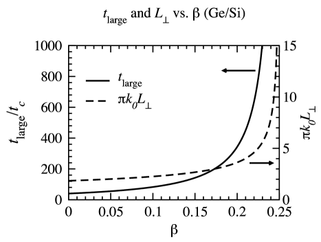
Figure 8: $t_{\text{large}}$ and $L_{\perp}$ vs. $\beta$ for Si/Ge using the 2D anisotropic model as described in Sec. 4. Units are normalize to characteristic time $t_{c}$ and predicted number of correlated dots ($n=k_{0}L_{\perp}/\pi$).

In [24] it was suggested that allowing the film to evolve with $\beta$ close to the stability threshold could enhance the SAQD correlation. It is interesting to note what happens for different values of $\beta$. Similar analytic and numerical calculations are performed for the large film-height limit, $\beta=0$, for the 2D anisotropic Ge/Si surface. For $\beta=0$, $t_{\text{large}}=40.3t_{c}$, $L_{\perp}=30.0\text{ nm}$, and $n=k_{0}L_{\perp}/\pi=1.84$, so one to two dots in a row are expected to be well correlated. $h(\mathbf{x})$ and real-space correlation functions are shown in Figs. 5g-i. The range of order is significantly less than for the case $\beta=0.208$ (Sec. 4.1). For Si/Ge at $600\text{K}$, the 2D anisotropic predictions for $t_{\text{large}}$ and $L_{\perp}$ are shown in Fig. 8. In general, the closer $\beta$ is to the critical value $0.25$, the longer the correlation length. One can manipulate equation (53) to find that $t_{\text{large}}/t_{c}$ varies approximately but not exactly as $(\beta-1/4)^{-1}\times\ln[h_{\text{large}}^{2}\sqrt{\epsilon_{A}}/(\Delta^{2}k_{c}^{2})]$. Consequently, $L_{\perp}\sim(\beta-1/4)^{-1/2}$. Furthermore, the appearance of $h_{\text{large}}$ and $\Delta^{2}$ inside the logarithm shows that the final order estimates are not overly sensitive to the guesses for $\Delta^{2}$ and $h_{\text{large}}^{2}$. The divergence of $L_{\perp}$ with $\beta-1/4$ is initially encouraging, but it is clear that for the parameters used for Ge/Si, subatomic control of the film height is needed to yield significantly enhanced long range correlations. Also as one approaches this threshold, one can probably expect thermal activation to nucleate subcritical SAQDs whose effect on supercritically formed SAQDs is uncertain. There should be some interesting phenomena at the the $0pt\rightarrow 0pt_{c}$.

5 Discussion/Conclusions

The order of epitaxial self-assembled quantum dots during initial stages of growth has been studied using a common model of surface diffusion with stochastic initial conditions. It has been shown that correlation functions of small surface height fluctuations can be predicted analytically using corresponding ensemble average correlation functions. These correlation functions are characterized by correlation lengths that can be predicted by analytic formulas given certain reasonable assumptions about the diffusion potential and the height and lateral scale of initial atomic scale random fluctuations. Thus, the linear model of film surface height evolution via surface diffusion has enabled analytic predictions of epitaxial SAQD order that are valid for small film height fluctuations. To what extent the initial degree of order persists into later stages of growth remains to be studied, but the order of initial stages should certainly have a strong influence on final outcomes. Furthermore, the linear analysis should provide insight into the less tractable non-linear behavior. These predictions of SAQD order have been used to investigate the role of crystal anisotropy and initial film height.

Crystal anisotropy has been shown to play an important role in enhancing SAQD order as observed in previous numerical simulations continuum and atomistic numerical simulations. [43, 37, 44, 45] If a four-fold symmetry is assumed for the governing dynamics, the effect of crystal anisotropy to linear order is felt through elastic anisotropy alone. It is shown that elastic anisotropy is required to produce a lattice-like structure of SAQDs. The enhanced spatial order should in turn lead to enhanced size order, a consequence that must be confirmed with non-linear studies, but appears to be true based on the present available literature.

The role of initial film height has been shown to greatly influence order. Growth near the critical film height for dot formation can enhance order. This order enhancement comes from increasing the duration of the linear small-fluctuation stage of growth. In fact, the predicted correlation lengths diverge when the initial film height approaches the critical film height from above. Achieving large correlation lengths in this manor is of course practically limited by ability to control film heights to subatomic accuracy. Additionally, one should be careful when interpreting the continuum model in such a context, as the effect of atomic discreteness might be greater at the transition film height. Finally, it is likely that additional randomizing effects of thermal activation will effectively cut off this divergence when the critical film height is approached from below during deposition.

Finally, the presented method may be useful as a first step in the analysis of methods to enhance SAQD order. It is reasonable to suppose that under some circumstances initial growth stages will be very important while for others they will not. For example, prior work on vertical stacking appears to confirm the presented ordering mechanism. [44]. Vertical stacking not only achieves vertical correlation of dots, but each layer is more ordered horizontally than the one below. Additionally, a “growth window” was found, whereby to achieve enhanced order, the evolution of each layer be terminated before ripening begins. The reported simulation [44] supports the following scenario for SAQD order development. Order is enhanced during the small fluctuation stage as described here. Once the fluctuations are sufficiently large, the seeded dots evolve towards their equilibrium shapes. Finally, the dots begin to ripen and order diminishes. Order is transfered via strain to the next layer so that the next layer gets a head start on its initial ordering. Thus, the multiple layers of dots effectively draws out the linear growth stage. It may be possible to modify the present model to predict the correlation length of each SAQD layer.

Appendix A Diffusion Potential

The diffusion potential is calculated in terms of the film height $0pt$ that is a function of the in plane coordinates $\mathbf{x}=x\mathbf{i}+y\mathbf{j}$. The elastic and surface energy portions of the diffusion potential can be found in [15]

$$\mu_{\text{elast}}(\mathbf{x})=\Omega\omega(\mathbf{x})\text{, and }\mu_{surf}=-\Omega\gamma\kappa(\mathbf{x}),$$

where $\Omega$ is the atomic volume, $\omega(\mathbf{x})$ is the elastic energy density at the film surface, $\gamma$ is the surface energy density, and $\kappa$ is the total surface curvature. However, other calculations need to be included:

1. $\mu_{\text{wet}}$ for the two wetting potential cases, Eq. (3) and (5),

2. and $\mu_{\text{surf}}$ and $\mu_{\text{wet}}$ when the surface energy density $\gamma$ and wetting energy density $W$ also depend on surface orientation.

Before these case are addressed, a general form for the diffusion potential is justified.

A.1 General Form $\mu=\Omega\delta\mathcal{F}/\delta 0pt(\mathbf{x})$

The diffusion potential, $\mu(\mathbf{x})$, is the change in free energy, $\mathcal{F}$, when a particle is added at a position, $\mathbf{x}$. Note that $\mu(\mathbf{x})$ and $\mathcal{F}$ are relative energies. They can be used to compare the binding energy of one site on the surface in comparison with another site, but should not be interpreted as an absolute binding energy or total formation energy of the surface. If a particle has a volume $\Omega$, then the diffusion potential at $\mathbf{x}$ is related to the variation of free energy with volume,

$$\delta\mathcal{F}=\Omega^{-1}\int d^{d}\mathbf{x}\,\mu(\mathbf{x})\delta V(\mathbf{x}),$$ (54)

where $\delta V(\mathbf{x})$ is the volume variation at $\mathbf{x}$. Calculating $\delta V(\mathbf{x})$, $V=\int d^{d}\mathbf{x}\,0pt(\mathbf{x}).$Therefore, $\delta V(\mathbf{x})=\delta 0pt(\mathbf{x}).$ Substituting into $\delta\mathcal{F}$ (Eq. (54)), $\delta\mathcal{F}=\Omega^{-1}\int d^{d}\mathbf{x}\,\mu(\mathbf{x})\delta 0pt(\mathbf{x})$ or $\mu(\mathbf{x})=\Omega\delta\mathcal{F}/\delta 0pt(\mathbf{x}).$

A.2 Simple Model

Starting from Eq. (2), $\mu(\mathbf{x})$ is found by taking the variational derivative,

$$\mu_{\text{elast.}}(\mathbf{x})=\Omega\frac{\delta}{\delta 0pt(\mathbf{x})}\int_{\text{volume}}d^{d}\mathbf{x}dz\,\omega[0pt](\mathbf{x},z)=\Omega\omega\left(\mathbf{x}\right)$$

where the “$[0pt]$” indicates that the elastic energy, $\omega$, is a nonlocal functional of the film height $0pt$, and $\omega(\mathbf{x})=\omega[0pt]\left(\mathbf{x},0pt(\mathbf{x})\right)$, the elastic energy density evaluated above lateral position $\mathbf{x}$ at the free surface ($z=0pt(\mathbf{x})$). See [15] for details of the derivation. The surface energy diffusion potential is

$$\mu_{\text{surf.}}(\mathbf{x,}t) = \Omega\frac{\delta}{\delta 0pt(\mathbf{x})}\int d^{d}\mathbf{x}\,\left[1+(\boldsymbol{\nabla}0pt(\mathbf{x}))^{2}\right]^{1/2}\gamma$$

$$= -\Omega\boldsymbol{\nabla}\cdot\left[1+(\boldsymbol{\nabla}0pt(\mathbf{x}))^{2}\right]^{1/2}\gamma=-\Omega\gamma\kappa(\mathbf{x}).$$

The wetting energy diffusion potential is

$$\mu_{\text{wet}}(\mathbf{x}) = \Omega\frac{\delta}{\delta 0pt(\mathbf{x})}\int d^{d}\mathbf{x}\,W(0pt(\mathbf{x}))$$

$$= \Omega W^{\prime}(0pt(\mathbf{x}))$$

Putting these three terms together, one obtains Eq. (3)

A.3 General Model

Consider the general form for the combined surface energy and wetting potential,

$$\mathcal{F}_{sw}=\int d^{d}\mathbf{x}\,F_{sw}(0pt(\mathbf{x}),\boldsymbol{\nabla}0pt(\mathbf{x}))$$

as in Eq. (2.1.1.2) so that the free energy is an integral over the $\mathbf{x}-$plane of an energy density that depends on $0pt(\mathbf{x})$ and $\boldsymbol{\nabla}0pt(\mathbf{x})$ locally. The corresponding diffusion potential is

$$\mu(\mathbf{x})=\Omega\frac{\delta\mathcal{F}_{sw}}{\delta 0pt(\mathbf{x})}=\Omega\left[F_{sw}^{(10)}(0pt(\mathbf{x}),\boldsymbol{\nabla}0pt(\mathbf{x}))-\boldsymbol{\nabla}\cdot\mathbf{F}_{sw}^{(10)}(0pt(\mathbf{x}),\boldsymbol{\nabla}0pt(\mathbf{x}))\right]$$

Appendix B Linearized Diffusion Potential and Anisotropy

The linearized diffusion potential $\mu_{\text{lin, }\mathbf{k}}$ is found by finding $\mu(\mathbf{x})$ to first order in height fluctuations ($h$), to get $\mu_{\text{lin}}(\mathbf{x})$ and then taking the Fourier transform to get $\mu_{\text{lin},\mathbf{k}}$. The linearization of the simple isotropic diffusion potential corresponding to Eqs. (2) and (3) was discussed in Sec. 2.1.1.1. Here, the more general diffusion potential corresponding to Eqs (2.1.1.2) and (5) is linearized and then applied to the anisotropic simple model and the anisotropic general model. Only the surface and wetting parts of the diffusion potential are discussed in this appendix. See ref. [15], Sec. 2.2.1.1 and Appendix C for discussion of $\mu_{\text{elast.}}$.

B.1 Linearizing the simple model

Consider a wetting potential and diffusion potential that both depend on the film height gradient $\boldsymbol{\nabla}0pt$, $\gamma\rightarrow\gamma(\boldsymbol{\nabla}0pt$) and $W(0pt)\rightarrow W(0pt,\boldsymbol{\nabla}0pt)$. Starting from Eq. (6) and expanding to second order in the film height fluctuation using $0pt(\mathbf{x})=\bar{0pt}+h(\mathbf{x})$ (Eq. (7)),

$$\left[1+\left(\boldsymbol{\nabla}0pt\right)^{2}\right]^{-1/2}\gamma(\boldsymbol{\nabla}0pt) = \left(1-\frac{1}{2}\left(\boldsymbol{\nabla}h\right)^{2}+\dots\right)\left(\gamma+\mathbf{\boldsymbol{\gamma}}^{\prime}\cdot\boldsymbol{\nabla}h+\tilde{\boldsymbol{\gamma}}^{\prime\prime}:\boldsymbol{\nabla}h\boldsymbol{\nabla}h+\dots\right)$$

$$= \gamma+\mathbf{\boldsymbol{\gamma}}^{\prime}\cdot\boldsymbol{\nabla}h-\frac{1}{2}\gamma\left(\boldsymbol{\nabla}h\right)^{2}+\tilde{\boldsymbol{\gamma}}^{\prime\prime}:\boldsymbol{\nabla}h\boldsymbol{\nabla}h+O[h^{3}]$$

where $\gamma$ is $\gamma(\mathbf{0})$, and the primes indicate the derivatives with respect to the surface height gradient.

$$\boldsymbol{\gamma}^{\prime}=\left.\partial_{\boldsymbol{\nabla}0pt}\gamma(\boldsymbol{\nabla}0pt)\right|_{\boldsymbol{\nabla}0pt=\mathbf{0}}\text{, and }\tilde{\boldsymbol{\gamma}}^{\prime\prime}=\left.\partial_{\boldsymbol{\nabla}0pt}\partial_{\boldsymbol{\nabla}0pt}\gamma(\boldsymbol{\nabla}0pt)\right|_{\boldsymbol{\nabla}0pt=\mathbf{0}}.$$

Taking the derivative with respect to $\boldsymbol{\nabla}h$ results in a tensor of rank equal to the order of the derivative because $\boldsymbol{\nabla}h$ is a vector (tank 1 tensor). Taking the variational derivative, $\mu_{\text{surf.}}(\mathbf{x})=\Omega\delta\mathcal{F}_{\text{surf.}}/\delta h(\mathbf{x})$,

$$\mu_{\text{surf., lin}}(\mathbf{x})=\Omega\left[\gamma\nabla^{2}h(\mathbf{x})-\tilde{\boldsymbol{\gamma}}^{\prime\prime}:\boldsymbol{\nabla}\boldsymbol{\nabla}h(\mathbf{x})\right]$$

The term with $\boldsymbol{\gamma}^{\prime}$ vanishes because it is the divergence of a constant ($\boldsymbol{\nabla}\cdot\boldsymbol{\gamma}^{\prime}$). Taking the inverse Fourier transform,

$$\mu_{\text{surf., lin},\mathbf{k}}=\Omega\left(-\gamma k^{2}+\mathbf{k}\cdot\tilde{\boldsymbol{\gamma}}^{\prime\prime}\cdot\mathbf{k}\right)h_{\mathbf{k}}.$$ (55)

The first term is isotropic. The second term is parameterized by a rank 2 symmetric tensor.

Going through the same process, one finds essentially the same result for an orientation dependent wetting energy. The step details are so close to the details for linearizing the more general form, $F_{sw}(0pt,\boldsymbol{\nabla}0pt)$, they are deferred to (Appendix B.2). One finds that

$$\mu_{\text{wet,lin},\mathbf{k}}=\Omega\left(W^{(20)}+\mathbf{k}\cdot\tilde{\mathbf{W}}^{(02)}\cdot\mathbf{k}\right).$$ (56)

where $W^{(mn)}=\left.\partial_{0pt}^{m}\partial_{\boldsymbol{\nabla}0pt}^{n}W(0pt,\boldsymbol{\nabla}0pt)\right|_{0pt=\bar{0pt},\boldsymbol{\nabla}0pt=\mathbf{0}}$ is the $m^{\text{th}}$ and $n^{\text{th}}$ derivative of the wetting energy density with respect to $0pt$ and $\boldsymbol{\nabla}0pt$ evaluated for a perfectly flat film of height $\bar{0pt}$. $W^{(mn)}$ is a tensor of rank $n$.

B.1.1 isotropic case

In the isotropic case, $\tilde{\boldsymbol{\gamma}}^{\prime\prime}\rightarrow\gamma^{\prime\prime}\tilde{\mathbf{I}}$, where $\tilde{\mathbf{I}}$ is the identity operator, and $\gamma^{\prime\prime}$ is a scalar. Similarly, $\tilde{\mathbf{W}}^{(02)}\rightarrow W^{(02)}\tilde{\mathbf{I}}$. One thus gets for the combined surface and wetting parts of the diffusion potential,

$$\mu_{sw,\text{lin},\mathbf{k}}=\Omega\left[\left(-\gamma+\gamma^{\prime\prime}+W^{(02)}\right)k^{2}+W^{(20)}\right]h_{\mathbf{k}}.$$

Thus, in the isotropic case, the linear order effect of introducing a surface orientation to either the surface energy or the wetting potential is simply to change the apparent surface energy density by $\gamma\rightarrow\gamma-\gamma^{\prime\prime}-W^{(02)}$.

B.1.2 anisotropic case

The surface and wetting parts of the diffusion potential (Eqs. (55) and (56)) can admit only a limited anisotropy. They both contain rank 2 symmetric tensors, $\tilde{\boldsymbol{\gamma}}^{\prime\prime}$ and $\tilde{\mathbf{W}}^{(02)}$ in the $\mathbf{x}-$plane. For a two-dimensional surface, this means that they can either have two-fold-symmetric (rotations by $180^{\circ}$) anisotropy or none at all. Thus, for the case considered in Sec. 2.2.1.2, four-fold-symmetric anisotropy , the surface and wetting parts of the diffusion potential must be completely isotropic. As discussed in Sec. 2.2.1.2, the (100) surface of zinc-blend structures, such as the mentioned Ge, Si, InAs and GaAs present a rather complicated situation. For simplicity, it is assumed here that the surface and wetting energies are at least four-fold symmetric. Consequently, they are completely isotropic.

Finally, it should be noted that if $F_{sw}$ depends on higher order derivatives, then the discussion is greatly complicated and a larger class of anisotropic terms is admissible. For example, when $F_{sw}\rightarrow F_{sw}(0pt,\boldsymbol{\nabla}0pt,\boldsymbol{\nabla}\boldsymbol{\nabla}0pt,\boldsymbol{\nabla}\boldsymbol{\nabla}\boldsymbol{\nabla}0pt,\dots)$ is expanded about $0pt(\mathbf{x})=\bar{0pt}$ to quadratic order in $h$, it would contains tensors of rank 6 and maybe even higher.

B.2 Linearizing the general model

The elastic part of the linearized diffusion potential was discussed in Sec. 2.2.1.1 and Appendix C . Eq. (56) can be found by using all of the following steps with the substitution $F_{sw}\rightarrow W$. The surface-wetting part of the diffusion potential $\mu(\mathbf{x})$ is found by expanding $F_{sw}$ to second order in the film-height fluctuation, $h$, and then taking the variational derivative. Expanding $F_{sw}$ about $h=0$ and $\boldsymbol{\nabla}h=\mathbf{0}$,

$$F_{sw}(\bar{0pt}+h,\boldsymbol{\nabla}h) = F_{sw}^{(00)}+F_{sw}^{(10)}h+\mathbf{F}_{sw}^{(01)}\cdot\boldsymbol{\nabla}h+{h\mathbf{F}}_{sw}^{(11)}\cdot\boldsymbol{\nabla}h\dots$$

$$\dots+\frac{1}{2}F_{sw}^{(20)}h^{2}+\frac{1}{2}\tilde{\mathbf{F}}_{sw}^{(02)}:\boldsymbol{\nabla}h\boldsymbol{\nabla}h+O[h^{3}].$$

Note that in this expansion, all the $F_{sw}^{(mn)}$ terms are constant with respect to $h$ and depend implicitly on the average film height, $\bar{0pt}$. The first index indicates the $m^{\text{th}}$ derivative with respect to $h$. The second index indicates the $n^{\text{th}}$ derivative with respect to $\boldsymbol{\nabla}h$. The derivatives are evaluated for a perfectly flat surface of height $\bar{0pt}$. Thus,

$$F_{sw}^{\left(mn\right)}=\left.\partial_{0pt}^{m}\partial_{\boldsymbol{\nabla}0pt}^{n}F_{sw}\left(0pt,\boldsymbol{\nabla}0pt\right)\right|_{0pt=\bar{0pt},\,\boldsymbol{\nabla}0pt=\mathbf{0}}.$$

Since $\boldsymbol{\nabla}h$ is a vector in the $\mathbf{x}-$plane, $F_{sw}^{(mn)}$ is a tensor of rank $n$. Taking the variational derivative of $\mathcal{F}_{sw}=\int d^{d}\mathbf{x}\,F_{sw}(0pt,\boldsymbol{\nabla}0pt)$ and keeping terms to order $h^{1}$,

$$\frac{\delta\mathcal{F}}{\delta h(\mathbf{x})}=F_{sw}^{(10)}-\boldsymbol{\nabla}\cdot\mathbf{F}_{sw}^{(01)}+F_{sw}^{(20)}h-\boldsymbol{\nabla}\cdot\left(\tilde{\mathbf{F}}_{sw}^{(02)}\cdot\boldsymbol{\nabla}h\right).$$

Note that the $F_{sw}^{(00)}$ term vanishes because it is constant, and the $\mathbf{F}_{sw}^{(11)}$ term vanishes upon simplification. Additionally, the $F_{sw}^{(10)}$ can be neglected if one enforces the condition that the film-height fluctuations do not add or subtract material from the surface, namely that $\int d^{d}\mathbf{x}\,\delta h(\mathbf{x},t)=0$. Alternatively, one can discard it in anticipation of taking the gradient of the diffusion potential, since it is a constant. The term $\boldsymbol{\nabla}\cdot\mathbf{F}_{sw}^{(01)}=0$ for the same reasons, or because $F_{sw}^{(01)}$ is a constant. Multiplying through by the atomic volume,

$$\mu_{\text{lin}}(\mathbf{x})=\Omega\left[F_{sw}^{(20)}h-\tilde{\mathbf{F}}_{sw}^{(02)}:\boldsymbol{\nabla}\boldsymbol{\nabla}h\right].$$ (57)

B.2.1 isotropic case

In the isotropic case, $\tilde{\mathbf{F}}_{sw}^{(02)}$ must be proportional to the identity so that $\tilde{\mathbf{F}}_{sw}^{(02)}=F_{sw}^{(02)}\tilde{\mathbf{I}}$; thus,

$$\mu_{sw,\text{lin}}(\mathbf{x})=\Omega\left[F_{sw}^{(20)}h(\mathbf{x})-F_{sw}^{(02)}\nabla^{2}h(\mathbf{x})\right].$$

Taking the inverse Fourier transform of this equation,

$$\mu_{sw,\text{lin},\mathbf{k}}=\Omega\left[F_{sw}^{(20)}+F_{sw}^{(02)}k^{2}\right]h_{\mathbf{k}}.$$

This gives case b in Eq. (9).

B.2.2 anisotropic case

If the surface is anisotropic, then $\tilde{\mathbf{F}}_{sw}^{(02)}$ in Eq. (57) is a rank 2 symmetric tensor in the $\mathbf{x}-$plane. Thus, it can have two distinct eigenvalues, and automatically has 2-fold rotational symmetry (rotations by $180^{\circ}$). If any other symmetry is assumed such as 4-fold symmetry (rotations by $90^{\circ}$), then $\tilde{\mathbf{F}}_{sw}^{(02)}$ must be fully isotropic. Taking the inverse Fourier transform,

$$\mu_{sw,\text{lin},\mathbf{k}}=\Omega\left[F_{sw}^{(20)}+\mathbf{k}\cdot\tilde{\mathbf{F}}_{sw}^{(02)}\cdot\mathbf{k}\right]h_{\mathbf{k}}.$$

In Eq. (23), case b, it is assumed that there is four-fold symmetry, resulting in a surface-wetting part of the diffusion potential that is completely isotropic.

Appendix C Elastic Anisotropy

In principal, the anisotropic elastic energy $\omega_{\mathbf{k}}$ is found in the same fashion as the isotropic elastic energy. [15] The flat film, initially in a state of biaxial stress, is perturbed by a small periodic surface fluctuation of amplitude $h_{0}$. An appropriate elastic field is added to satisfy the perturbed traction-free boundary condition at the free surface. Finally, the elastic energy is evaluated at the free surface to first order in $h_{0}$. The coefficient $h_{0}$ is the sought after $\omega_{\mathbf{k}}$. The equations themselves are cumbersome and best solved using a numeric implementation, so an abstract procedure for calculating $\omega_{\mathbf{k}}$ is outlined here. $\omega_{\mathbf{k}}$ is found for $k=1$ but arbitrary $\theta_{\mathbf{k}}$.

Let the surface have a height variation

$$h(\mathbf{x})=h_{0}e^{ikx}.$$

To first order in $h_{0}$, the surface normal is

$$\mathbf{n}(\mathbf{x})=-ikh_{0}e^{ikx}\mathbf{i}+\mathbf{k}.$$

The elastic energy needs to be calculated to first order in $h_{0}$. To find the elastic energy, it is necessary to find the perturbing elastic field to first order in $h_{0}$.

The initial unperturbed stress state is

$$\tilde{\sigma}_{m}=\left[\begin{array}[]{ccc}\sigma_{m}&0&0\\ 0&\sigma_{m}&0\\ 0&0&0\end{array}\right],$$

where $\sigma_{m}=\left(c_{11}+c_{12}-2c_{12}^{2}/c_{11}\right)\epsilon_{m}$. Note that this stress state is isotropic in the $x-y$-plane and thus independent of rotations about the vertical axis. Under this stress state, a flat surface is traction-free. With the height perturbation, the traction is

$$t_{j}=\left(\mathbf{n}\cdot\tilde{\sigma}_{m}\right)_{j}=-ikh_{0}M\epsilon_{m}\delta_{j1}e^{ikx}.$$ (58)

Next to find the perturbing elastic fields. These are not isotropic in the $x-y-$plane, and it is necessary to take into account the angle. First, the $3\times 3\times 3\times 3$ elastic stiffness tensor $c_{ijkl}$ is constructed for the cube orientation from the compact $9\times 9$ matrix $c_{ij}$. The tensor representation aids in rotation. The stiffness tensor is then passively rotated in the $x-y-$plane by an angel $\theta_{\mathbf{k}}$,

$$c_{ijkl}(\theta_{\mathbf{k}})=\sum_{m,n,p,q=1}^{3}R(\theta_{\mathbf{k}})_{im}R(\theta_{\mathbf{k}})_{jn}R(\theta_{\mathbf{k}})_{kp}R(\theta_{\mathbf{k}})_{lq}c_{mnpq}$$

where

$$R(\theta_{\mathbf{k}})=\left[\begin{array}[]{ccc}\cos(\theta_{\mathbf{k}})&\sin(\theta_{\mathbf{k}})&0\\ -\sin(\theta_{\mathbf{k}})&\cos(\theta_{\mathbf{k}})&0\\ 0&0&1\end{array}\right].$$

This passive rotation of $c_{ijkl}$ is equivalent to actively rotating the wave vector $\mathbf{k}=k\mathbf{i}$ by $\theta_{\mathbf{k}}$.

The appropriate form for the perturbing displacement field is found. Assume a displacement of the form

$$u_{i}(x,y,z)=U_{i}e^{k(ix+\kappa z)},$$

where $\kappa$ can have a complex value. The elastic equilibrium equations are

$$\sum_{i,k,l=1}^{3}\frac{\partial}{\partial x_{i}}c_{ijkl}(\theta_{\mathbf{k}})\frac{\partial}{\partial x_{k}}u_{l}=0;\,j=1\dots 3.$$

$$\left(\sum_{l=1}^{3}C_{jl}(\theta_{\mathbf{k}},\kappa)U_{l}\right)k^{2}e^{k(ix+\kappa z)}=0$$ (59)

where

$$C_{jl}(\theta_{\mathbf{k}},\kappa)=\sum_{i,k=1}^{3}c_{ijkl}(\theta_{\mathbf{k}})(i\delta_{i1}+\delta_{i3}\kappa)(i\delta_{k1}+\delta_{k3}\kappa).$$

Factoring out $k^{2}e^{k(ix+\kappa z)}$, the part in parenthesis must be identically zero.

To obtain a non-trivial solution, the determinant of $C_{jl}(\theta_{\mathbf{k}},\kappa)$ to zero. Six complex values of $\kappa$ are found. The values of $\kappa$ with $\text{Re}[\kappa]<0$ are discarded since the corresponding displacements blow up as $z\rightarrow-\infty$. Each of the remaining values $\kappa=\kappa^{p}$ with $p=1\dots 3$ is substituted back into $C_{jl}(\theta_{\mathbf{k}},\kappa)$, and Eq. (59) is solved to find the corresponding eigenvectors, $U_{l}^{p}$. The total displacement is thus

$$u_{l}(x,y,z)=i\epsilon_{m}h_{0}\sum_{p=1}^{3}A_{p}U_{l}^{p}e^{k(ix+\kappa^{p}z)},$$

where it is assumed that the perturbing elastic displacement field is proportional to $h_{0}$and $\sigma_{m}$, and the factor of $i$ is put in for convenience. The coefficients $A_{p}$ can be found from the traction-free boundary condition at the free surface. The traction formula is

$$t_{j} = \sum_{i,k,l=1}^{3}n_{i}c_{ijkl}(\theta_{\mathbf{k}})\frac{\partial}{\partial x_{k}}u_{l}(x,y,z)=ik\epsilon_{m}h_{0}\sum_{i,k,l,p=1}^{3}n_{i}c_{ijkl}(\theta_{\mathbf{k}})A_{p}U_{l}^{p}(i\delta_{k1}+\kappa^{p}\delta_{k3})e^{k(ix+\kappa^{p}z)}$$ (60)

The traction is already proportional to $h_{0}$. Thus, all terms in the sum must be kept to zeroth order in $h_{0}$ so that

$$h(\mathbf{x})=0\text{, and }\mathbf{n}(\mathbf{x})=\mathbf{k}.$$

Thus, plugging $z=0$ to Eq. (60),

$$t_{j}=ik\epsilon_{m}h_{0}\sum_{p=1}^{3}\sum_{l=1}^{3}\left(ic_{3j1l}(\theta_{\mathbf{k}})+\kappa^{p}c_{3j3l}(\theta_{\mathbf{k}})\right)A_{p}U_{l}^{p}e^{ikx}.$$ (61)

Since the total traction (Eqs. (58) and (61)) must be zero, the coefficients $A_{p}$ are found from

$$K_{jp}A_{p}=R_{j},$$

where

$$K_{jp}=\sum_{l=1}^{3}\left(ic_{3j1l}(\theta_{\mathbf{k}})+\kappa^{p}c_{3j3l}(\theta_{\mathbf{k}})\right)U_{l}^{p},$$

and

$$R_{j}=M\delta_{j1}$$

for $j=1\dots 3$. It is worth noting that only for the symmetry directions, $\theta_{\mathbf{k}}=0^{\circ}$ and $\theta_{\mathbf{k}}=45^{\circ}$ is the strain purely plane-strain as it is for the elastically isotropic case.

The elastic energy at the film surface is found to order $O(h_{0})$. If the stress and strain are expanded to first order in $h_{0}$, $\tilde{\sigma}=\tilde{\sigma}_{0}+\tilde{\sigma}_{1}$, and $\tilde{\epsilon}=\tilde{\epsilon}_{0}+\tilde{\epsilon}_{1}$, then

$$U=\frac{1}{2}\tilde{\epsilon}:\tilde{c}:\tilde{\epsilon}=\frac{1}{2}\tilde{\sigma}_{0}:\epsilon_{0}+\tilde{\sigma}_{0}:\tilde{\epsilon}_{1}+O(h_{0}^{2}).$$

Thus,

$$U=U_{0}+M\epsilon_{m}\left((\epsilon_{1})_{11}+(\epsilon_{1})_{22}\right)$$

$$(\epsilon_{1})_{11}=\frac{\partial u_{1}}{\partial x}=-\epsilon_{m}kh_{0}\sum_{p=1}^{3}A_{p}U_{1}^{p}.$$

$(\epsilon_{1})_{22}=\partial u_{2}/\partial y=0$. Thus,

$$U=U_{0}-\mathcal{E}_{\theta_{\mathbf{k}}}kh_{0}e^{ikx}$$

where

$$\mathcal{E}_{\theta_{\mathbf{k}}}=M\epsilon_{m}^{2}\sum_{p=1}^{3}A_{p}U_{1}^{p}$$

where $A_{p}$and $U_{1}^{p}$ are implicitly functions of $\theta_{\mathbf{k}}$. This procedure has been used to find the values of $\mathcal{E}_{0^{\circ}}$ and $\mathcal{E}_{45^{\circ}}$ for Table. 2 and Sec. 4.

Appendix D Diffusional Anisotropy

In general, the surface diffusivity can depend on the film height $0pt(\mathbf{x})$ and the surface orientation $\boldsymbol{\nabla}0pt(\mathbf{x})$ so that the surface current is

$$\mathbf{J}_{S}(\mathbf{x})=\tilde{\mathbf{D}}(0pt(\mathbf{x}),\boldsymbol{\nabla}H(\mathbf{x}))\cdot\boldsymbol{\nabla}s\mu(\mathbf{x})$$

where $\boldsymbol{\nabla}s$ is the surface gradient, and $\tilde{\mathbf{D}}$ is a rank 2 tensor in the two-dimensional space tangent to the film surface at $\mathbf{x}$. Linearizing the surface current about a flat surface,

$$\mathbf{J}_{S}(\mathbf{x})=\tilde{\mathbf{D}}(\bar{0pt})\cdot\boldsymbol{\nabla}\mu_{\text{lin}}(\mathbf{x})$$

where the diffusivity must be evaluated for $h=0$ and $\boldsymbol{\nabla}h=0$, since $\mu_{\text{lin}}(\mathbf{x})$ is already proportional to $h(\mathbf{x})$. The linearized diffusivity is a symmetric rank 2 tensor in the $\mathbf{x}-$plane. Thus, it is similar to $\tilde{\mathbf{F}}_{sw}$ discussed in Appendix B.2.2. It is automatically either two-fold symmetry (rotations by $180^{\circ}$) or it is completely isotropic. In Eq. (23), four-fold symmetry of the surface is assumed. Thus, the diffusivity must be completely isotropic; $\tilde{\mathbf{D}}\rightarrow\mathcal{D}$, a scalar. Section 2.2.1.2 and Appendix B.2.2 contain discussions of the symmetry properties of the various rank 2 tensors that appear in the linear evolution equations. A limited case of diffusional anisotropy has been modeled via kinetic Monte Carlo technique. [54]

Appendix E Correlation Functions

E.1 Mean Values

Equations (31) and (33) are central to the presented analysis. Here, they are derived. The two-point correlation functions for a stochastic system are introduced. Then, the average of the autocorrelation function is taken and expressed in terms of the two-point correlation functions. Finally, this average is simplified using the translational invariance of the system (governing equations and ensemble of initial conditions).

The two-point real-space space correlation function is

$$C(\mathbf{x},\mathbf{x}^{\prime})=\left\langle h(\mathbf{x})h(\mathbf{x}^{\prime})^{*}\right\rangle,$$

and the reciprocal space correlation function is

$$C_{\mathbf{k}\mathbf{k}^{\prime}}=\left\langle h_{\mathbf{k}}h_{\mathbf{k}^{\prime}}^{*}\right\rangle.$$

These are related by the double Fourier transform,

$$C_{\mathbf{k}\mathbf{k}^{\prime}}=\frac{1}{(2\pi)^{2d}}\int d^{d}\mathbf{x}d^{d}\mathbf{x}^{\prime}\,e^{-i\mathbf{k}\cdot\mathbf{x}+i\mathbf{k}^{\prime}\cdot\mathbf{x}^{\prime}}C(\mathbf{x},\mathbf{x}^{\prime});$$ (62)

$$C(\mathbf{x},\mathbf{x}^{\prime})=\int d^{d}\mathbf{k}d^{d}\mathbf{k}^{\prime}\,e^{i\mathbf{k}\cdot\mathbf{x}-i\mathbf{k}^{\prime}\cdot\mathbf{x}^{\prime}}C_{\mathbf{k}\mathbf{k}^{\prime}}.$$ (63)

These ensemble correlation functions can be used to give the ensemble-mean autocorrelation function and spectrum function. In real space,

$$\left\langle C^{A}(\boldsymbol{\Delta}\mathbf{x})\right\rangle = \frac{1}{A}\int d^{2}\mathbf{x}^{\prime}\,\left\langle h(\boldsymbol{\Delta}\mathbf{x}+\mathbf{x}^{\prime})h(\mathbf{x}^{\prime})\right\rangle$$ (64)

$$= \frac{1}{A}\int d^{2}\mathbf{x}^{\prime}\,C(\boldsymbol{\Delta}\mathbf{x}+\mathbf{x}^{\prime},\mathbf{x}^{\prime}).$$

$$\left\langle C_{\mathbf{k}}^{A}\right\rangle=\frac{(2\pi)^{d}}{A}\left\langle h_{\mathbf{k}}h_{\mathbf{k}}^{*}\right\rangle=\frac{(2\pi)^{d}}{A}C_{\mathbf{k}\mathbf{k}}.$$ (65)

Fortunately, the translational invariance of the system simplifies these relations. Inspecting the governing equations and invoking the translational invariance of the stochastic initial conditions, the resulting ensemble and its statistical measures must also be translationally invariant. Thus under the translation by $\mathbf{x}^{\prime}$,

$$C(\boldsymbol{\Delta}\mathbf{x}+\mathbf{x}^{\prime},\mathbf{x}^{\prime})=C(\boldsymbol{\Delta}\mathbf{x},\mathbf{0})=C(\boldsymbol{\Delta}\mathbf{x}),$$ (66)

so that the independent variable is reduced to just the difference vector $\boldsymbol{\Delta}\mathbf{x}=\mathbf{x}-\mathbf{x}^{\prime}$. This relation can be used to simplify both the real and reciprocal space relations.

The real space relation simplifies as follows.Inserting Eq. (66) into Eq. (64),

$$\left\langle C^{A}(\boldsymbol{\Delta}\mathbf{x})\right\rangle=\frac{1}{A}\int d^{2}\mathbf{x}^{\prime}\,C(\boldsymbol{\Delta}\mathbf{x},\mathbf{0})=C(\boldsymbol{\Delta}\mathbf{x}).$$ (67)

The reciprocal space relation (Eq. (62)) simplifies to

$$C_{\mathbf{k}\mathbf{k}^{\prime}}=C_{\mathbf{k}}\delta^{2}(\mathbf{k}-\mathbf{k}^{\prime})=C_{\mathbf{k}}\frac{A}{(2\pi)^{d}}\delta_{\mathbf{k}\mathbf{k}^{\prime}},$$ (68)

where

$$C_{\mathbf{k}}=\frac{1}{(2\pi)^{d}}\int d^{2}\boldsymbol{\Delta}\mathbf{x}\,e^{-i\mathbf{k}\cdot\boldsymbol{\Delta}\mathbf{x}}C(\boldsymbol{\Delta}\mathbf{x}).$$

One can see immediately from Eq. (67) that $C_{\mathbf{k}}$ is the Fourier transform of $\left\langle C^{A}(\boldsymbol{\Delta}\mathbf{x})\right\rangle=C(\boldsymbol{\Delta}\mathbf{x})$, or one can plug Eq. (68) into Eq. (65), to get $\left\langle C_{\mathbf{k}}^{A}\right\rangle=C_{\mathbf{k}}.$

E.2 Variance and Convergence

The ergodic hypothesis is that an average with respect to a parameter such as position or time tends towards an ensemble average. In this case,

$$C_{\mathbf{k}}^{A}\approx\left\langle C_{\mathbf{k}}^{A}\right\rangle=C_{\mathbf{k}},$$ (69)

and $$C^{A}(\boldsymbol{\Delta}\mathbf{x})\approx\left\langle C^{A}(\boldsymbol{\Delta}\mathbf{x})\right\rangle=C(\boldsymbol{\Delta}\mathbf{x}).$$

when the surface area is very large. The ensemble average is a good substitute if the variance about the average vanishes as the substrate area $A$ becomes large. It is found that in reciprocal space,

$$\text{Var}(C_{\mathbf{k}}^{A})=\left\langle\left(C_{\mathbf{k}}^{A}\right)^{2}\right\rangle-\left\langle C_{\mathbf{k}}^{A}\right\rangle^{2}=C_{\mathbf{k}}^{2}.$$ (70)

Thus, the ergodic hypothesis does not hold for $C_{\mathbf{k}}^{A}$. In practice, $C_{\mathbf{k}}^{A}$ is a speckled version of $C_{\mathbf{k}}$ (Fig. 6) However, if one smooths $C_{\mathbf{k}}^{A}$ by averaging over a small patch in reciprocal space of size $k_{\text{smooth}}=1/\Delta_{s}$, so that

$$C_{\mathbf{k}}^{A}(\Delta_{s})=\left(\frac{\Delta_{s}^{2}}{2\pi}\right)^{d/2}\int d^{d}\mathbf{k}^{\prime}\,e^{-\frac{1}{2}\Delta_{s}^{2}(\mathbf{k}^{\prime}-\mathbf{k})^{2}}C_{\mathbf{k}^{\prime}}^{A},$$ (71)

then $\text{Var}\left(C_{\mathbf{k}}^{A}(\Delta_{s})\right)$ diminishes as $1/A$. For sufficiently large $\Delta_{s}$,

$$\left\langle C_{\mathbf{k}}^{A}(\Delta_{s})\right\rangle\approx C_{\mathbf{k}},$$ (72)

and

$$\text{Var}\left(C_{\mathbf{k}}^{A}(\Delta_{s})\right)\approx\frac{\pi^{d/2}\Delta_{s}^{d}}{A}C_{\mathbf{k}}^{2}.$$ (73)

Thus, the ergodic hypothesis (Eq. (69)) only holds for a smoothed version of $C_{\mathbf{k}}^{A}$.

In real space,

$$\text{Var}\left(C^{A}(\boldsymbol{\Delta}\mathbf{x})\right) = \left\langle\left(C^{A}(\boldsymbol{\Delta}\mathbf{x})\right)^{2}\right\rangle-\left\langle C^{A}(\boldsymbol{\Delta}\mathbf{x})\right\rangle^{2}$$ (74)

$$= \frac{(2\pi)^{d}}{A}\int d^{d}\mathbf{k}\,\left(e^{2i\mathbf{k}\cdot\boldsymbol{\Delta}\mathbf{x}}C_{\mathbf{k}}^{2}+C_{\mathbf{k}}^{2}\right),$$

where the integral is bounded (finite) provided that either $t>0$ or the atomic scale cutoff $b_{0}>0$. Thus, the ergodic hypothesis holds for the real space autocorrelation function.

E.2.1 Eq. (70)

First, $\left\langle C_{\mathbf{k}}^{A}C_{\mathbf{k}^{\prime}}^{A}\right\rangle$ is calculated.

$$\left\langle C_{\mathbf{k}}^{A}C_{\mathbf{k}^{\prime}}^{A}\right\rangle=\left(\frac{(2\pi)^{d}}{A}\right)^{2}\left\langle h_{\mathbf{k}}h_{\mathbf{k}}^{*}h_{\mathbf{k}^{\prime}}h_{\mathbf{k}^{\prime}}^{*}\right\rangle.$$

Assume that he distribution of $h_{\mathbf{k}}$ is gaussian. Also, assume that $h(\mathbf{x})$ is real so that $h_{\mathbf{k}}h_{-\mathbf{k}}=\left|h_{\mathbf{k}}\right|^{2}$. Then,

$$\left\langle h_{\mathbf{k}_{1}}h_{\mathbf{k}_{2}}^{*}h_{\mathbf{k}_{3}}h_{\mathbf{k}_{4}}^{*}\right\rangle = C_{\mathbf{k}_{1}}C_{\mathbf{k}_{2}}\delta^{d}(\mathbf{k}_{1}-\mathbf{k}_{4})\delta^{d}(\mathbf{k}_{2}-\mathbf{k}_{3})\dots$$

$$\dots +C_{\mathbf{k}_{1}}C_{\mathbf{k}_{2}}\delta^{d}(\mathbf{k}_{1}+\mathbf{k}_{3})\delta^{d}(\mathbf{k}_{2}+\mathbf{k}_{4})\dots$$

$$\dots +C_{\mathbf{k}_{1}}C_{\mathbf{k}_{3}}\delta^{d}(\mathbf{k}_{1}-\mathbf{k}_{2})\delta^{d}(\mathbf{k}_{3}-\mathbf{k}_{4}).$$

Thus,

$$\left\langle C_{\mathbf{k}}^{A}C_{\mathbf{k}^{\prime}}^{A}\right\rangle = \left(\frac{(2\pi)^{d}}{A}\right)^{2}\left(C_{\mathbf{k}}^{2}\left[\delta^{d}(\mathbf{k}-\mathbf{k}^{\prime})\right]^{2}\dots\right.$$ (75)

$$\dots\left.+C_{\mathbf{k}}^{2}\left[\delta^{d}(\mathbf{k}+\mathbf{k}^{\prime})\right]^{2}+C_{\mathbf{k}}C_{\mathbf{k}^{\prime}}\left[\delta^{d}(\mathbf{0})\right]^{2}\right).$$

$$= C_{\mathbf{k}}^{2}\left(\delta_{\mathbf{k}\mathbf{k}^{\prime}}+\delta_{\mathbf{k}(-\mathbf{k}^{\prime})}\right)+C_{\mathbf{k}}C_{\mathbf{k}^{\prime}},$$ (76)

where Eq. (29) has been used liberally. Setting $\mathbf{k}=\mathbf{k}^{\prime}$, results in Eq. (70).

E.2.2 Eq. (73)

Now consider $C_{\mathbf{k}}^{A}$ smoothed over a length $\Delta_{s}$ (Eq. (71)). The mean value is

$$\left\langle C_{\mathbf{k}}^{A}(\Delta_{s})\right\rangle = \left(\frac{\Delta_{s}^{2}}{2\pi}\right)^{d/2}\int d^{d}\mathbf{k}^{\prime}\,e^{-\frac{1}{2}\Delta_{s}^{2}(\mathbf{k}^{\prime}-\mathbf{k})^{2}}\left\langle C_{\mathbf{k}^{\prime}}^{A}\right\rangle.$$

$$= \left(\frac{\Delta_{s}^{2}}{2\pi}\right)^{d/2}\int d^{d}\mathbf{k}^{\prime}\,e^{-\frac{1}{2}\Delta_{s}^{2}(\mathbf{k}^{\prime}-\mathbf{k})^{2}}C_{\mathbf{k}^{\prime}}.$$

For sufficiently small $k_{\text{smooth}}$, (sufficiently large $\Delta_{s}$), Eq. (72) results.

The variance of $C_{\mathbf{k}}^{A}(\Delta_{s})$ is now calculated. First, it is necessary to calculate $\left\langle\left[C_{\mathbf{k}}^{A}(\Delta_{s})\right]^{2}\right\rangle$.

$$\left\langle\left[C_{\mathbf{k}}^{A}(\Delta_{s})\right]^{2}\right\rangle = \left(\frac{\Delta_{s}^{2}}{2\pi}\right)^{d}\int d^{d}\mathbf{k}^{\prime}\,e^{-\frac{1}{2}\Delta_{s}^{2}(\mathbf{k}^{\prime}-\mathbf{k})^{2}}\dots$$

$$\dots \times\int d^{d}\mathbf{k}^{\prime\prime}\,e^{-\frac{1}{2}\Delta_{s}^{2}(\mathbf{k}^{\prime\prime}-\mathbf{k})^{2}}\left\langle C_{\mathbf{k}^{\prime}}^{A}C_{\mathbf{k}^{\prime\prime}}^{A}\right\rangle.$$

Using Eq. (75) and Eq. (29) as needed,

$$\left\langle\left[C_{\mathbf{k}}^{A}(\Delta_{s})\right]^{2}\right\rangle = \left(\frac{\Delta_{s}^{2}}{2\pi}\right)^{d}\int d^{d}\mathbf{k}^{\prime}d^{d}\mathbf{k}^{\prime\prime}\,e^{-\frac{1}{2}\Delta_{s}^{2}(\mathbf{k}^{\prime}-\mathbf{k})^{2}}e^{-\frac{1}{2}\Delta_{s}^{2}(\mathbf{k}^{\prime\prime}-\mathbf{k})^{2}}\left(\frac{(2\pi)^{d}}{A}\right)^{2}\dots$$

$$\dots\times\left\{C_{\mathbf{k}}^{2}\left[\delta^{d}(\mathbf{k}^{\prime}-\mathbf{k}^{\prime\prime})\right]^{2}+C_{\mathbf{k}}^{2}\left[\delta^{d}(\mathbf{k}^{\prime}+\mathbf{k}^{\prime\prime})\right]^{2}+C_{\mathbf{k}}C_{\mathbf{k}^{\prime}}\left[\delta^{d}(\mathbf{0})\right]^{2}\right\}$$

$$= \frac{\Delta_{s}^{2d}}{A}\int d^{d}\mathbf{k}^{\prime}\,\left\{e^{-\Delta_{s}^{2}(\mathbf{k}^{\prime}-\mathbf{k})^{2}}C_{\mathbf{k}^{\prime}}^{2}+e^{-\frac{1}{2}\Delta_{s}^{2}\left[(\mathbf{k}^{\prime}-\mathbf{k})^{2}+(\mathbf{k}^{\prime}+\mathbf{k})^{2}\right]}C_{\mathbf{k}^{\prime}}^{2}\right\}\dots$$

$$\dots+\left[\left(\frac{\Delta_{s}^{2}}{2\pi}\right)^{d/2}\int d^{d}\mathbf{k}^{\prime}\,e^{-\frac{1}{2}\Delta_{s}^{2}(\mathbf{k}^{\prime}-\mathbf{k})^{2}}C_{\mathbf{k}^{\prime}}\right]^{2}$$

The first integral is bounded (finite) because $C_{\mathbf{k}}$ is bounded. Let its finite value be denoted $I$. The second integral is simply $\left\langle C_{\mathbf{k}}^{A}(\Delta_{s})\right\rangle.$Thus,

$$\text{Var}(C_{\mathbf{k}}^{A}(\Delta_{s}))=\frac{\Delta_{s}^{2d}I}{A},$$

a finite value that decreases as $A^{-1}$ as required for the ergodic hypothesis to hold. For sufficiently small $k_{\text{smooth }}$ (large $\Delta_{s}$), $I\approx(\pi/\Delta_{s}^{2})^{d/2}C_{\mathbf{k}}^{2}$, and Eq. (73) results. It should also be noted that the large $\Delta_{s}$ required for this approximation also creates a more stringent requirement that $A$ be large.

E.2.3 Eq. (74)

Now, consider the real space auto-correlation function. First, $\left\langle C^{A}(\boldsymbol{\Delta}\mathbf{x})C^{A}(\boldsymbol{\Delta}\mathbf{x})\right\rangle$ is needed.

$$\left\langle C^{A}(\boldsymbol{\Delta}\mathbf{x})C^{A}(\boldsymbol{\Delta}\mathbf{x})\right\rangle=\int d^{d}\mathbf{k}d^{d}\mathbf{k}^{\prime}\,e^{i(\mathbf{k}+\mathbf{k}^{\prime})\cdot\boldsymbol{\Delta}\mathbf{x}}\left\langle C_{\mathbf{k}}^{A}C_{\mathbf{k}^{\prime}}^{A}\right\rangle$$

Proceeding in a fashion similar to the previous section (making use of Eqs. (75) and (29) as needed) ,

$$\left\langle C^{A}(\boldsymbol{\Delta}\mathbf{x})C^{A}(\boldsymbol{\Delta}\mathbf{x})\right\rangle = \frac{(2\pi)^{2d}}{A^{2}}\int d^{d}\mathbf{k}d^{d}\mathbf{k}^{\prime}\,e^{i(\mathbf{k}+\mathbf{k}^{\prime})\cdot\boldsymbol{\Delta}\mathbf{x}}\left(C_{\mathbf{k}}^{2}\left[\delta^{d}(\mathbf{k}-\mathbf{k}^{\prime})\right]^{2}\dots\right.$$

$$\left.\dots+C_{\mathbf{k}}^{2}\left[\delta^{d}(\mathbf{k}+\mathbf{k}^{\prime})\right]^{2}+C_{\mathbf{k}}C_{\mathbf{k}^{\prime}}\left[\delta^{d}(\mathbf{0})\right]^{2}\right)$$

$$= \frac{(2\pi)^{d}}{A}\int d^{d}\mathbf{k}\,\left(e^{2i\mathbf{k}\cdot\boldsymbol{\Delta}\mathbf{x}}C_{\mathbf{k}}^{2}+C_{\mathbf{k}}^{2}\right)\dots$$

$$\dots+\left(\int d^{d}\mathbf{k}\,e^{i\mathbf{k}\cdot\boldsymbol{\Delta}\mathbf{x}}C_{\mathbf{k}}\right)\left(\int d^{d}\mathbf{k}^{\prime}\,e^{i\mathbf{k}^{\prime}\cdot\boldsymbol{\Delta}\mathbf{x}}C_{\mathbf{k}}\right)$$

$$= \frac{(2\pi)^{d}}{A}\int d^{d}\mathbf{k}\,\left(e^{2i\mathbf{k}\cdot\boldsymbol{\Delta}\mathbf{x}}C_{\mathbf{k}}^{2}+C_{\mathbf{k}}^{2}\right)+\left\langle C^{A}(\boldsymbol{\Delta}\mathbf{x})\right\rangle^{2}$$

Thus, Eq. (74) results. For the variance to be vanishing, the integral in Eq. (74) must be bounded (finite). If time, $t>0$, the exponential in Eq. (77) guarantees that the integral is bounded. For time $t=0$, the integral is only bounded if the atomic scale cutoff $b_{0}>0$.

Appendix F Atomic Scale Cutoff

Starting from Eq. (39),

$$C_{\mathbf{k}}=\frac{\Delta^{2}}{(2\pi)^{d}}e^{2\sigma_{\mathbf{k}}t-\frac{1}{2}b_{0}^{2}k^{2}}.$$ (77)

The effect of the small scale cutoff is both small and short-lived, as it only works to suppress fluctuations with large wavenumbers. The most important fluctuations have wavenumbers between $0$ and $2k_{c}$. Thus, the typical size of the cutoff term is about $b_{0}^{2}k_{c}^{2}.$ If a typical dot size or spacing size $10\text{ nm}$, and a typical atomic scale is $10^{-1}\text{ nm}$, a typical value for this term is about $10^{-3}-10^{-2}$. To calculate the effect of the cutoff, it can absorbed into the time-dependent part with the substitution

$$b\rightarrow b\left(1+\frac{b_{0}^{2}}{4b\mathcal{D}t}\right)$$

so that its effect lasts only as long as a perturbation with atomic scale curvature ($\kappa=b_{0}$). Thus, Eq. (40) is a good approximation.

References

- [1] D. Bimberg, M. Grnudmann, and N. N. Ledentsov. Quantum Dot Heterostructures. John Wiley & Sons, 1999.
- [2] O. P. Pchelyakov, Yu. B. Bolkhovityanov, A. V. Dvurechenski, L. V. Sokolov, A. I. Nikiforov, A. I. Yakimov, and B. Voigtländer. SiliconGermanium nanostructures with quantum dots: Formation mechanisms and electrical properties. Semiconductors, 34(11):122947, 2000. [doi:10.1134/1.1325416].
- [3] M. Grundmann. The present status of quantum dot lasers. Physica E, 5:167, 2000. [doi:10.1016/S1386-9477(99)00041-7].
- [4] Pierre M. Petroff, Axel Lorke, and Atac Imamoglu. Epitaxially self-assembled quantum dots. Physics Today, pages 46–52, May 2001.
- [5] Hui-Yun Liu, Bo Xu, Yong-Qiang Wei, Ding Ding, Jia-Jun Qian, Qin Han, Ji-Ben Liang, and Zhan-Guo Wang. High-power and long-lifetime InAs/GaAs quantum-dot laser at 1080 nm. Applied Physics Letters, 79(18):2868–70, 2001. [doi:10.1063/1.1415416].
- [6] F. Heinrichsdorff, M.H. Mao, N. Kirstaedter, A. Krost, D. Bimberg, A. O. Kosogov, and P. Werner. Room-temperature continuous-wave lasing from stacked InAs/GaAs quantum dots grown by metalorganic chemical vapor deposition. Applied Physics Letters, 71(1):22–4, 1997. [doi:doi:10.1063/1.120556].
- [7] D. Bimberg, N.N. Ledentsov, and J.A. Lott. Quantum-dot vertical-cavity surface-emitting laser. MRS Bulletin, 27(7):531–7, 2002.
- [8] N. N. Ledentsov. Long-wavelength quantum-dot lasers on GaAs substrates: From media to device concepts. IEEE Journal of Selected Topics in Quantum Electronics, 8(5):1015–23, September/October 2002. [doi:10.1109/JSTQE.2002.804236].
- [9] M Friesen, P Rugheimer, D. E. Savage, M. G. Lagally, D. W. van der Weide, R Joynt, and M. A. Eriksson. Practical design and simulation of silicon-based quantum-dot qubits. Physical Review B, 67(12):121301 (R), 2003. [doi:10.1103/PhysRevB.67.121301].
- [10] Yi-Chang Cheng, San-Te (Cing-Ming) Yang, Jyh-Neng Yang, Liann-Be Chang, and Li-Zen Hsieh. Fabrication of a far-infrared photodetector based on InAs/GaAs quantum-dot superlattices. Optical Engineering, 42(1):11923, 2003. [doi:doi:10.1117/1.1525277].
- [11] R. Krebs, S. Deubert, J.P. Reithmaier, and A. Forchel. Improved performance of MBE grown quantum-dot lasers with asymmetricdots in a well design emitting near 1.3 m. Journal of Crystal Growth, 251:7427, 2003. [doi:10.1016/S0022-0248(02)02385-0].
- [12] Hiroyuki Sakaki. Progress and prospects of advanced quantum nanostructures and roles of molecular beam epitaxy. Journal of Crystal Growth, 251:9–16, 2003. [doi:10.1016/S0022-0248(03)00831-5].
- [13] B. J. Spencer, P. W. Voorhees, and S. H. Davis. Morphological instability in epitaxially strained dislocation-free films. Physical Review Letters, 67(26):3696–3699, 1991. [doi:10.1103/PhysRevLett.67.3696].
- [14] Karl Brunner. Si/ge nanostructures. Reports on Progress in Physics, 65(1):27–72, 2002. [doi:10.1088/0034-4885/65/1/202].
- [15] L. B. Freund and S. Suresh. Thin Film Materials: Stress, Defect Formation and Surface Evolution, chapter 8. Cambridge University Press, 2003.
- [16] S. Yu Shiryaev, E. Verstlund Pedersen, F. Jensen, J. Wulff Petersen, J. Lundsgaard Hansen, and A. Nylandsted Larson. Dislocation patterning - a new tool for spatial manipulation of Ge islands. Thin solid films, 294(1-2):311–314, 1997. [doi: 10.1016/S0040-6090(96)09240-1].
- [17] C. Kumar and L. H. Friedman. Simulation of thermal field directed self assembly of epitaxial self-assembled Ge quantum dots. Journal of Applied Physics, in press.
- [18] Lawrence H. Friedman and Jian Xu. Feasibility study for thermal-field directed self-assembly of heteroepitaxial quantum dots. Applied Physics Letters, 88:093105, 2006. [doi:10.1063/1.2179109].
- [19] S. Krishna, D. Zhu, J. Xu, and P. Bhattacharya. Structural and luminescence characteristics of cycled submonolayer InAs/GaAs quantum dots with room-temperature emission at 1.3 m. Journal of Applied Physics, 86:6135–8, 1999. [doi:10.1063/1.371664].
- [20] R. Hull, J.L. Gray, M. Kammler, T. Vandervelde, T. Kobayashi, P. Kumar, T. Pernell, J.C. Bean, J.A. Floro, and F.M. Ross. Precision placement of heteroepitaxial semiconductor quantum dots. Materials Science and Engineering B, 101:1–8, 2003. [doi:10.1016/S0921-5107(02)00680-3].
- [21] O. Guise, Jr. J. T. Yates, J. Levy, J. Ahner, V. Vaithyanathan, and D. G. Schlom. Patterning of sub-10nm ge islands on si(100) by direct self-assembly. Applied Physics Letters, 87:171902, 2005. [doi:10.1063/1.2112198].
- [22] X. Niu, R. Vardavas, R. E. Caflisch, and C. Ratsch. Level set simulation of directed self-assembly during epitaxial growth. Physical Review B, 74(19):193403, Nov 2006. [doi:10.1103/PhysRevB.74.193403.
- [23] Z. M. Zhao, T. S. Yoon, W. Feng, B. Y. Li, J. H. Kim, J. Liu, O. Hulko, Y. H. Xie, H. M. Kim, K. B. Kim, H. J. Kim, K. L. Wang, C. Ratsch, R. Caflisch, D. Y. Ryu, and T. P. Russell. The challenges in guided self-assembly of ge and inas quantum dots on si. THIN SOLID FILMS, 508(1-2):195–199, Jun 2006. [doi:10.1016/j.tsf.2005.08.407].
- [24] Lawrence H. Friedman. Anisotropy and order of epitaxial self-assembled quantum dots. Physical Review B, in press.
- [25] Y. Obayashi and K. Shintani. Directional dependence of surface morphological stability of heteroepitaxial layers. Journal of Applied Physics, 84(6):3141, 1998. [doi:10.1063/1.368468].
- [26] C. S. Ozkan, W. D. Nix, and H. J. Gao. Stress-driven surface evolution in heteroepitaxial thin films: Anisotropy of the two-dimensional roughening mode. JOURNAL OF MATERIALS RESEARCH, 14(8):3247–3256, Aug 1999. [doi:10.1557/JMR.1999.043].
- [27] J. Tersoff and F. K. LeGoues. Competing relaxation mechanisms in strained layers. Physical Review Letters, 72(22):3570–3573, May 1994. [doi:10.1103/PhysRevLett.72.3570].
- [28] B. J. Spencer, P. W. Voorhees, and S. H. Davis. Morphological instability in epitaxially strained dislocation-free solid films: Linear stability theory. Journal of Applied Physics, 73(10):4955–4970, 1993. [doi: 10.1063/1.353815].
- [29] J. M. Baribeau, X. Wu, N. L. Rowell, and D. J. Lockwood. Ge dots and nanostructures grown epitaxially on si. JOURNAL OF PHYSICS-CONDENSED MATTER, 18(8):R139–R174, Mar 2006. [doi:10.1088/0953-8984/18/8/R01].
- [30] D. J. Srolovitz. On the stability of surfaces of stressed solids. Acta Metallurgica, 37(2):621–625, 1989. [doi:10.1016/0001-6160(89)90246-0].
- [31] H. J. Gao and W. D. Nix. Surface roughening of heteroepitaxial thin films. ANNUAL REVIEW OF MATERIALS SCIENCE, 29:173–209, 1999. [doi:0.1146/annurev.matsci.29.1.173].
- [32] P. Sutter and M. G. Lagally. Nucleationless three-dimensional island formation in low-misfit heteroepitaxy. Physical Review Letters, 84(20):4637, 2000. [doi:10.1103/PhysRevLett.84.4637.
- [33] A. A. Golovin, S. H. Davis, and P. W. Voorhees. Self-organization of quantum dots in epitaxially strained solid films. Physical Review E, 68:056203, 2003. [doi:10.1103/PhysRevE.68.056203].
- [34] A. Ramasubramaniam and V. B. Shenoy. Growth and ordering of si-ge quantum dots on strain patterned substrates. JOURNAL OF ENGINEERING MATERIALS AND TECHNOLOGY-TRANSACTIONS OF THE ASME, 127(4):434–443, Oct 2005. [doi:10.1115/1.1924559].
- [35] I. Berbezier, A. Ronda, F. Volpi, and A. Portavoce. Morphological evolution of SiGe layers. Surface Science, 531:231–243, 2003. [doi:10.1016/S0039-6028(03)00488-6].
- [36] J. R. R. Bortoleto, H. R. Gutierrez, M. A. Cotta, J. Bettini, L. P. Cardoso, and M. M. G. de Carvalho. Spatial ordering in InP/InGaP nanostructures. Applied Physics Letters, 82(20):3523–3525, 2003. [doi:10.1063/1.1572553].
- [37] P. Liu, Y. W. Zhang, and C. Lu. Formation of self-assembled heteroepitaxial islands in elastically anisotropic films. Physical Review B, 67:165414, 2003. [doi: 10.1103/PhysRevB.67.165414].
- [38] Y.W. Zhang, A.F. Bower, and P. Liu. Morphological evolution driven by strain induced surface diffusion. Thin solid films, 424:9–14, 2003. [doi:10.1016/S0040-6090(02)00897-0].
- [39] Yu U. Wang, Yongmei M. Jin, and Armen G. Khachaturyan. Phase field microelasticity modeling of surface instability of heteroepitaxial thin films. Acta Materialia, 52:81–92, 2004. [doi:10.1016/j.actamat.2003.08.027].
- [40] W. T. Tekalign and B. J. Spencer. Evolution equation for a thin epitaxial film on a deformable substrate. Journal of Applied Physics, 96(10):5505–5512, 2004. [doi:10.1063/1.1766084].
- [41] M. J. Beck, A. van de Walle, and M. Asta. Surface energetics and structure of the ge wetting layer on si(100). Physical Review B, 70(20):205337, Nov 2004. [doi:10.1103/PhysRevB.70.205337].
- [42] Y. H. Tu and J. Tersoff. Origin of apparent critical thickness for island formation in heteroepitaxy. Physical Review Letters, 93(21):216101, Nov 2004. [doi:10.1103/PhysRevLett.93.216101.
- [43] V. Holy, G. Springholz, M. Pinczolits, and G. Bauer. Strain induced vertical and lateral correlations in quantum dot superlattices. Physical Review Letters, 83(2):356–359, 1999. [doi:10.1103/PhysRevLett.83.356].
- [44] P. Liu, Y. W. Zhang, and C. Lu. Three-dimensional finite-element simulations of the self-organized growth of quantum dot superlattices. Physical Review B, 68:195314, 2003. [doi:10.1103/PhysRevB.68.195314].
- [45] G. Springholz, M. Pinczolits, V. Holy, S. Zerlauth, I. Vavra, and G. Bauer. Vertical and lateral ordering in self-organized quantum dot superlattices. Physica E, 9:149–163, 2001. [doi:10.1016/S1386-9477(00)00189-2.
- [46] P. Liu, Y. W. Zhang, and C. Lu. Coarsening kinetics of heteroepitaxial islands in nucleationless stranski-krastanov growth. Physical Review B, 68:035402, 2003. [doi:10.1103/PhysRevB.68.035402].
- [47] F. M. Ross, J. Tersoff, and R. M. Tromp. Coarsening of self-assembled ge quantum dots on Si(001). Physical Review Letters, 80(5):984–7, 1998. [doi:10.1103/PhysRevLett.80.984].
- [48] J. Tersoff. Kinetic surface segregation and the evolution of nanostructures. Applied Physics Letters, 83(2):353–355, 2003. [doi:doi:10.1063/1.1592304].
- [49] A. Ramasubramaniam and V. B. Shenoy. A spectral method for the nonconserved surface evolution of nanocrystalline gratings below the roughening transition. Journal of Applied Physics, 97(11):114312, 2005. [doi: 10.1063/1.1897837].
- [50] Y. W. Zhang and A. F. Bower. Three-dimensional analysis of shape transitions in strained-heteroepitaxial islands. Applied Physics Letters, 78(18):2706–2708, 2001. [doi:10.1063/1.1354155].
- [51] L. E. Vorbyev. Handbook Series On Semiconductor Parameters, volume 1. World Scientific, 1996.
- [52] A. A. Golovin, M. S. Levine, T. V. Savina, and S. H. Davis. Faceting instability in the presence of wetting interactions: A mechanism for the formation of quantum dots. Physical Review B, 70:235342, 2004. [doi:10.1103/PhysRevB.70.235342].
- [53] B L Liang, Zh M Wang, Yu I Mazur, V V Strelchuck, K Holmes, J H Lee, and G J Salamo. Ingaas quantum dots grown on b-type high index gaas substrates: surface morphologies and optical propertiesmorphologies and optical properties. Nanotechnology, 17(11):2736–2740, 2006. [doi:10.1088/0957-4484/17/11/004].
- [54] M. Meixner, R. Kunert, and E. Scholl. Control of strain-mediated growth kinetics of self-assembled semiconductor quantum dots. Physical Review B, 67:195301, 2003. [doi: 10.1103/PhysRevB.67.195301].
- [55] Robert Zwanzig. Nonequilbrium Statistical Mechanics. Oxford University Press, New York, 2001.
- [56] C. W. Gardiner. Handbook of Stochastic Methods for Physics Chemistry and the Natural Sciences. Springer, New York, 3rd edition, 2004.
- [57] M. C. Cross and P. C. Hohenberg. Pattern formation outside equilibrium. Reviews of Modern Physics, 65(3):851–1112, 1993. [doi:10.1103/RevModPhys.65.851].
- [58] B. J. Spencer, S. H. Davis, and P. W. Voorhees. Morphological instability in epitaxially strained dislocation-free solid films: Nonlinear evolution. Physical Review B, 47(15):9760, 1993. [doi: 10.1103/PhysRevB.47.9760].