On-line Viterbi Algorithm and Its Relationship to Random Walks

Abstract

In this paper, we introduce the on-line Viterbi algorithm for decoding hidden Markov models (HMMs) in much smaller than linear space. Our analysis on two-state HMMs suggests that the expected maximum memory used to decode sequence of length $n$ with $m$-state HMM can be as low as $\Theta(m\log n)$, without a significant slow-down compared to the classical Viterbi algorithm. Classical Viterbi algorithm requires $O(mn)$ space, which is impractical for analysis of long DNA sequences (such as complete human genome chromosomes) and for continuous data streams. We also experimentally demonstrate the performance of the on-line Viterbi algorithm on a simple HMM for gene finding on both simulated and real DNA sequences.

Keywords:

hidden Markov models, on-line algorithms, Viterbi algorithm, gene finding

1 Introduction

Hidden Markov models (HMMs) are generative probabilistic models that have been succesfuly used for annotation of sequence data, such as DNA and protein sequences, natural langauge texts, and sequences of observations or measurements. Their numerous applications include gene finding [1], protein secondary structure prediction [2], and speech recognition [3]. The linear-time Viterbi algorithm [4] is the most commonly used algorithm for these tasks. Unfortunately, the space required by the Viterbi algorithm grows linearly with the length of the sequence (with a high constant factor), which makes it unsuitable for analysis of continuous or very long sequences. For example, DNA sequence of a single chromosome can be hundreds of megabases long. In this paper, we address this problem by proposing an on-line Viterbi algorithm that on average requires much less memory and that can annotate continuous streams of data on-line without reading the complete input sequence first.

An HMM, composed of states and transitions, is a probabilistic model that generates sequences over a given alphabet. In each step of this generative process, the current state generates one symbol of the sequence according to the emission probabilities associated with that state. Then, an outgoing transition is randomly chosen according to the transition probability table, and this transition is followed to the new state. This process is repeated until the whole sequence is generated.

The states in the HMM represent distinct features of the observed sequences (such as protein coding and non-coding sequences in a genome), and the emission probabilities in each state represent statistical properties of these features. The HMM thus defines a joint probability $\Pr(X,S)$ over all possible sequences $X$ and all state paths $S$ through the HMM that could generate these sequences. To annotate a given sequence $X$, we want to recover the state path $S$ that maximizes this joint probability. For example, in an HMM with one state for protein-coding sequences, and one state for non-coding sequences, the most probable state path marks each symbol of the input sequence $X$ as either protein coding or non-coding.

To compute the most probable state path, we use the Viterbi dynamic programming algorithm [4]. For every prefix $X_{1}\dots X_{i}$ of the given sequence $X$ and for every state $j$, we compute the most probable state path generating this prefix ending in state $j$. We store the probability of this path in table $P(i,j)$ and its second last state in table $B(i,j)$. These values can be computed from left to right, using the recurrence $P(i,j)=\max_{k}\{P(i-1,k)\cdot t_{k}(j)\cdot e_{j}(X_{i})\}$, where $t_{k}(j)$ is the transition probability from state $k$ to state $j$, and $e_{j}(X_{i})$ is the emission probability of the $i$-th symbol of X in state $j$. Back pointer $B(i,j)$ is the value of $k$ that maximizes $P(i,j)$. After computing these values, we can recover the most probable state path $S=s_{1},\allowbreak{}\dots,\allowbreak{}s_{n}$ by setting the last state as $s_{n}=\arg\max_{k}\{P(n,k)\}$, and then following the back pointers $B(i,j)$ from right to left (i.e., $s_{i}=B(i+1,s_{i+1})$). For an HMM with $m$ states and a sequence $X$ of length $n$, the running time of the Viterbi algorithm is $\Theta(nm^{2})$, and the space is $\Theta(nm)$.

This algorithm is well suited for sequences and models of moderate size. However, to annotate all 250 million symbols of the human chromosome 1 with a gene finding HMM consisting of hundred states, we would require 25 GB of memory just to store the back pointers $B(i,j)$. This is clearly impractical on most computational platforms.

Several solutions are used in practice to overcome this problem. For example, most practical gene finding programs process only sequences of limited size. The long input sequence is split into several shorter sequences which are processed separately. Afterwards, the results are merged and conflicts are resolved heuristically. This approach leads to suboptimal solutions, especially if the genes we are looking for cross the boundaries of the split.

Grice et al. [5] proposed a practical checkpointing algorithm that trades running time for space. We divide the input sequence into $K$ blocks of $L$ symbols, and during the forward pass, we only keep the first column of each block. To obtain the most probable state path, we recompute the last block of $L$ columns, and use back pointers to recover the last $L$ states of the most probable path, as well as the last state of the previous block. The information about this last state can now be used to recompute the most probable state path within the previous block in the same way, and the process is repeated for all blocks. Since every value of $P(i,j)$ will be computed twice, this means two-fold slow-down compared to the Viterbi algorithm, but if we set $K=L=\sqrt{n}$, this algorithm only requires $\Theta(\sqrt{n}m)$ memory. Checkpointing can be further generalized to trade $L$-fold slow-down for memory of $\Theta(\sqrt[L]{n}m)$ [6, 7].

In this paper, we propose and analyze an on-line Viterbi algorithm that does not use fixed amount of memory for a given sequence. Instead, the amount of memory varies depending on the properties of the HMM and the input sequence. In the worst case, our algorithm still requires $\Theta(nm)$ memory; however, in practice the requirements are much lower. We prove, by demonstrating analogy to random walks and using results from the theory of extreme values, that in simple cases the expected space for a sequence of length $n$ is as low as $\Theta(m\log n)$. We also experimentally demonstrate that the memory requirements are low for more complex HMMs.

2 On-line Viterbi algorithm

In our algorithm, we represent the back pointer matrix $B$ in the Viterbi algorithm by a tree structure (see [4]), with node $(i,j)$ for each sequence position $i$ and each state $j$. Parent of node $(i,j)$ is the node $(i-1,B(i,j))$. In this data structure, the most probable state path is a path from the leaf node $(n,j)$ with the highest probability $P(n,j)$ to the root of the tree (see Figure 1).

This tree is built as the Viterbi algorithm progresses from left to right. After processing sequence position $i$, all edges that do not lie on one of the paths ending in a level $i$ node can be removed; these edges will not be used in the most probable path [8]. The remaining $m$ paths represent all possible initial segments of the most probable state path. These paths are not necessarily edge disjoint; in fact, often all the paths share the same prefix up to some node called coalescence point (see Figure 1).

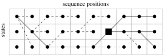
Figure 1: Example of the back pointer tree structure. Dashed lines mark the edges that cannot be part of the most probable state path. The square node marks the coalescence point of the remaining paths.

Left of the coalescence point, there is only a single candidate for the initial segment of the most probable state path. Therefore we can output this segment and remove all edges and nodes of the tree up to the coalescence point. Forney [4] describes an algorithm that after processing $D$ symbols of the input sequence checks whether a coalescence point has been reached; in such case, the initial segment of the most probable state path is outputted. If the coalescence point was not reached, one potential initial segment is chosen heuristicaly. Several studies [9, 10] suggest how to choose $D$ to limit the expected error caused by such heuristic steps in the context of convolution codes.

Here we show how to detect the existence of a coalescence point dynamically without introducing significant overhead to the whole computation. We maintain a compressed version of the back pointer tree, where we omit all internal nodes that have less than two children. Any path consisting of such nodes will be contracted to a single edge. This compressed tree has $m$ leaves and at most $m-1$ internal nodes. Each node stores the number of its children and a pointer to its parent node. We also keep a linked list of all the nodes of the compressed tree ordered by the sequence position. Finally, we also keep the list of pointers to all the leaves.

When processing the $k$-th sequence position in the Viterbi algorithm, we update the compressed tree as follows. First, we create a new leaf for each node at position $i$, link it to its parent (one of the former leaves), and insert it into the linked list. Once these new leaves are created, we remove all the former leaves that have no children, and recursively all of their ancestors that would not have any children.

Finally, we need to compress the new tree: we examine all the nodes in the linked list in order of decreasing sequence position. If the node has zero or one child and is not a current leaf, we simply delete it. For each leaf or node that has at least two children, we follow the parent links until we find its first ancestor (if any) that has at least two children and link the current node directly to that ancestor. A node $(\ell,j)$ that does not have an ancestor with at least two children is the coalescence point; it will become a new root. We can output the most probable state path for all sequence positions up to $\ell$, and remove all results of computation for these positions from memory.

The running time of this update is $O(m)$ per sequence position, and the representation of the compressed tree takes $O(m)$ space. Thus the asymptotic running time of the Viterbi algorithm is not increased by the maintanance of the compressed tree. Moreover, we have implemented both the standard Viterbi algorithm and our new on-line extension, and the time measurements suggest that the overhead required for the compressed tree updates is less than 5%.

The worst-case space required by this algorithm is still $O(nm)$. However, this is rarely the case for realistic data; required space changes dynamically depending on the input. In the next section, we show that for simple HMMs the expected maximum space required for processing sequence of length $n$ is $\Theta(m\log n)$. This is much better than checkpointing, which requires space of $\Theta(m\sqrt{n})$ with a significant increase in running time. We conjecture that this trend extends to more complex cases. We also present experimental results on a gene finding HMM and real DNA sequences showing that the on-line Viterbi algorithm leads to significant savings in memory.

Another advantage of our algorithm is that it can construct initial segments of the most probable state path before the whole input sequence is read. This feature makes it ideal for on-line processing of signal streams (such as sensor readings).

3 Memory requirements of the on-line Viterbi algorithm

In this section, we analyze the memory requirements of the on-line Viterbi algorithm. The memory used by the algorithm is variable throughout the execution of the algorithm, but of special interest are asymptotic bounds on the expected maximum amount of memory used by the algorithm while decoding a sequence of length $n$.

We use analogy to random walks and results in extreme value theory to argue that for a symmetric two-state HMMs, the expected maximum memory is $\Theta(m\log n)$. We also conduct experiments on an HMM for gene finding, and both real and simulated DNA sequences.

3.1 Symmetric two-state HMMs

Consider a two-state HMM over a binary alphabet as shown in Figure 2a. For simplicity, we assume $t<1/2$ and $e<1/2$. The back pointers between the sequence positions $i$ and $i+1$ can form one of the configurations i–iii shown in Figure 2b. Denote $p_{A}=\log P(i,A)$ and $p_{B}=\log P(i,B)$, where $P(i,j)$ is the table of probabilities from the Viterbi algorithm. The recurrence used in the Viterbi algorithm implies that the configuration i occurs when $\log t-\log(1-t)\leq p_{A}-p_{B}\leq\log(1-t)-\log t$, configuration ii occurs when $p_{A}-p_{B}\geq\log(1-t)-\log t$, and configuration iii occurs when $p_{A}-p_{B}\leq\log t-\log(1-t)$. Configuration iv never happens for $t<1/2$.

Figure 2: (a) Symmetric two-state HMM with two parameters: $e$ for emission probabilities and $t$ for transitions probabilities. (b) Possible back-pointer configurations for the two-state HMM.

Note that for a two-state HMM, a coalescence point occurs whenever one of the configurations ii or iii occur. Thus the memory used by the HMM is proportional to the length of continuous sequence of configurations i. We will call such a sequence of configurations a run.

First, we analyze the length distribution of runs under the assumption that the input sequence $X$ is a sequence of uniform i.i.d. binary random variables. In such case, we represent the run by a symmetric random walk corresponding to a random variable $X=\frac{p_{A}-p_{B}}{\log(1-e)-\log e}-(\log t-\log(1-t)).$ Whenever this variable is within the interval $(0,K)$, where $K=\left\lceil 2\frac{\log(1-t)-\log(t)}{\log(1-e)-\log(e)}\right\rceil,$ the configuration i occurs, and the quantity $p_{A}-p_{B}$ is updated by $\log(1-e)-\log e$, if the symbol at the corresponding sequence position is 0, or $\log e-\log(1-e)$, if this symbol is 1. These shifts correspond to updating the value of $X$ by $+1$ or $-1$.

When $X$ reaches 0, we have a coalescence point in configuration iii, and the $p_{A}-p_{B}$ is initialized to $\log t-\log(1-t)\pm(\log e-\log 1-e)$, which either means initialization of $X$ to $+1$, or another coalescence point, depending on the symbol at the corresponding sequence position. The other case, when $X$ reaches $K$ and we have a coalescence point in configuration ii, is symmetric.

We can now apply the classical results from the theory of random walks (see [11, ch.14.3,14.5]) to analyze the expected length of runs.

Lemma 1

Assuming that the input sequence is uniformly i.i.d., the expected length of a run of a symmetrical two-state HMM is $K-1$.

Therefore the larger is $K$, the more memory is required to decode the HMM. The worst case is achieved as $e$ approaches $1/2$. In such case, the two states are indistinguishable and being in state $A$ is equivalent to being in state $B$. Using the theory of random walks, we can also characterize the distribution of length of runs.

Lemma 2

Let $R_{\ell}$ be the event that the length of a run of a symmetrical two-state HMM is either $2\ell+1$ or $2\ell+2$. Then, assuming that the input sequence is uniformly i.i.d., for some constants $b,c>0$:

$$b\cdot\cos^{2\ell}\frac{\pi}{K}\leq\Pr(R_{\ell})\leq c\cdot\cos^{2\ell}\frac{\pi}{K}$$ (1)

Proof

For a symmetric random walk on interval $(0,K)$ with absorbing barriers and with starting point $z$, the probability of event $W_{z,n}$ that this random walk ends in point $0$ after $n$ steps is zero, if $n-z$ is odd, and the following quantity, if $n-z$ is even [11, ch.14.5]:

$$\Pr(W_{z,n})=\frac{2}{K}\sum_{0<v<K/2}\cos^{n-1}\frac{\pi v}{K}\sin\frac{\pi v}{K}\sin\frac{\pi zv}{K}$$ (2)

Using symmetry, note that the probability of the same random walk ending after $n$ steps at barrier $K$ is the same as probability of $W_{K-z,n}$. Thus, if $K$ is odd, we can state:

$$\Pr(R_{\ell}) = \Pr(W_{1,2\ell+1})+\Pr(W_{K-1,2\ell+1})$$ (3)

$$= \frac{2}{K}\sum_{0<v<K/2}\cos^{2\ell}\frac{\pi v}{K}\sin\frac{\pi v}{K}\left(\sin\frac{\pi v}{K}+(-1)^{v+1}\sin\frac{\pi v}{K}\right)$$

$$= \frac{4}{K}\sum_{0<v<K/2,\mbox{ $v$ odd}}\cos^{2\ell}\frac{\pi v}{K}\sin^{2}\frac{\pi v}{K}$$

There are at most $K/4$ terms in the sum and they can all be bounded from above by $\cos^{2\ell}\frac{\pi v}{K}$. Thus, we can give both upper and lower bounds on $\Pr(R_{\ell})$ using only the first term of the sum as follows:

$$\frac{4}{K}\sin^{2}\frac{\pi}{K}\cos^{2\ell}\frac{\pi}{K}\leq\Pr(R_{\ell})\leq\cos^{2\ell}\frac{\pi}{K}$$ (4)

Similarly, if $K$ is even, we can state:

$$\Pr(R_{\ell}) = \Pr(W_{1,2\ell+1})+\Pr(W_{K-1,2\ell+2})$$ (5)

$$= \frac{2}{K}\sum_{0<v<K/2}\cos^{2\ell}\frac{\pi v}{K}\sin^{2}\frac{\pi v}{K}\left(1+(-1)^{v+1}\cos\frac{\pi v}{K}\right)$$

and thus we have a similar bound:

$$\frac{2}{K}\sin^{2}\frac{\pi}{K}\left(1+\cos\frac{\pi}{K}\right)\cos^{2\ell}\frac{\pi}{K}\leq\Pr(R_{\ell})\leq 2\cos^{2\ell}\frac{\pi}{K}$$ (6)

∎

The previous lemma characterizes the length distribution of a single run. However, to analyze memory requirements for a sequence of length $n$, we need to consider maximum over several runs whose total length is $n$. Similar problem was studied for the runs of heads in a sequence of $n$ coin tosses [12, 13]. For coin tosses, the length distribution of runs is geometric, while in our case the runs are only bounded by geometricaly decaying functions. Still, we can prove that the expected length of the longest run grows logarithmically with the length of the sequence, as is the case for the coin tosses.

Lemma 3

Let $X_{1},X_{2},\dots$ be a sequence of i.i.d. random variables drawn from a geometrically decaying distribution over positive integers, i.e. there exist constants $a,b,c$, $a\in(0,1)$, $0<b\leq c$, such that for all integers $k\geq 1$, $ba^{k}\leq\Pr(X_{i}>k)\leq ca^{k}.$

Let $N_{n}$ be the largest index such that $\sum_{i=1\dots N_{n}}X_{i}\leq n$, and let $Y_{n}$ be $\max\{X_{1},X_{2},\dots,X_{N_{n}},n-\sum_{i=1}^{N_{n}}X_{i}\}$. Then

$$E[Y_{n}]=\log_{1/a}n+o(\log n)$$ (7)

Proof

Let $Z_{n}=\max_{i=1\dots n}X_{n}$ be the maximum of the first $n$ runs. Clearly, $\Pr(Z_{n}\leq k)=\Pr(X_{i}\leq k)^{n}$, and therefore $(1-ca^{k})^{n}\leq\Pr(Z_{n}\leq k)\leq(1-ba^{k})^{n}$ for all integers $k\geq\log_{1/a}(c)$.

Lower bound:

Let $t_{n}=\log_{1/a}n-\sqrt{\ln n}$. If $Y_{n}\leq t_{n}$, we need at least $n/t_{n}$ runs to reach the sum $n$, i.e. $N_{n}\geq n/t_{n}-1$ (discounting the last incomplete run). Therefore

$$\Pr(Y_{n}\leq t_{n})\leq\Pr(Z_{\frac{n}{t_{n}}-1}\leq t_{n})\leq(1-ba^{t_{n}})^{\frac{n}{t_{n}}-1}=(1-ba^{t_{n}})^{a^{-t_{n}}a^{t_{n}}(\frac{n}{t_{n}}-1)}$$ (8)

Since $\lim_{n\to\infty}a^{t_{n}}(n/t_{n}-1)=\infty$ and $\lim_{x\to 0}(1-bx)^{1/x}=e^{-b}$, we get $\lim_{n\to\infty}\Pr(Y_{n}\leq t_{n})=0$. Note that $E[Y_{n}]\geq t_{n}(1-\Pr(Y_{n}\leq t_{n}))$, and thus we get the desired bound.

Upper bound:

Clearly, $Y_{n}\leq Z_{n}$ and so $E[Y_{n}]\leq E[Z_{n}]$. Let $Z^{\prime}_{n}$ be the maximum of $n$ i.i.d. geometric random variables $X^{\prime}_{1},\dots,X^{\prime}_{n}$ such that $\Pr(X^{\prime}_{i}\leq k)=1-a^{k}$.

We will compare $E[Z_{n}]$ to the expected value of variable $Z^{\prime}_{n}$. Without loss of generality, $c\geq 1$. For any real $x\geq\log_{1/a}(c)+1$ we have:

$$\Pr(Z_{n}\leq x) \geq (1-ca^{\lfloor x\rfloor})^{n}$$

$$= \left(1-a^{\lfloor x\rfloor-\log_{1/a}(c)}\right)^{n}$$

$$\geq \left(1-a^{\lfloor x-\log_{1/a}(c)-1\rfloor}\right)^{n}$$

$$= \Pr(Z^{\prime}_{n}\leq x-\log_{1/a}(c)-1)$$

$$= \Pr(Z^{\prime}_{n}+\log_{1/a}(c)+1\leq x)$$

This inequality holds even for $x<\log_{1/a}(c)+1$, since the right-hand side is zero in such case. Therefore, $E[Z_{n}]\leq E[Z^{\prime}_{n}+\log_{1/a}(c)+1]=E[Z^{\prime}_{n}]+O(1)$. Expected value of $Z^{\prime}_{n}$ is $\log_{1/a}(n)+o(\log n)$ [14], which proves our claim.∎

Using results of Lemma 3 together with the characterization of run length distributions by Lemma 2, we can conclude that for symmetric two-state HMMs, the expected maximum memory required to process a uniform i.i.d. input sequence of length $n$ is $(1/\ln(1/\cos(\pi/K)))\cdot\ln n+o(\log n)$. Using the Taylor expansion of the constant term as $K$ grows to infinity, $1/\ln(1/\cos(\pi/K)))=2K^{2}/\pi^{2}+O(1)$, we obtain that the maximum memory grows approximately as $(2K^{2}/\pi^{2})\ln n$.

The asymptotic bound $\Theta(\log n)$ can be easily extended to the sequences that are generated by the symmetric HMM, instead of uniform i.i.d. The underlying process can be described as a random walk with approximately $2K$ states on two $(0,K)$ lines, each line corresponding to sequence symbols generated by one of the two states. The distribution of run lengths still decays geometrically as required by Lemma 3; the base of the exponent is the largest eigenvalue of the transition matrix with absorbing states omitted (see e.g. [15, Claim 2]).

The situation is more complicated in the case of non-symmetric two-state HMMs. Here, our random walks proceed in steps that are arbitrary real numbers, different in each direction. We are not aware of any results that would help us to directly analyze distributions of runs in these models, however we conjecture that the size of the longest run is still $\Theta(\log n)$. Perhaps, to obtain bounds on the length distribution of runs, one can approximate the behaviour of such non-discrete random walks by a different model (for example, [16, ch.7]).

3.2 Multi-state HMMs

Our analysis technique cannot be easily extended to HMMs with many states. In two-state HMMs, each new coalescence event clears the memory, and thus the execution of the algorithm can be divided into more or less independent runs. A coalescent event in a multi-state HMM results in a non-trivial tree left in memory, sometimes with a substantial depth. Thus, the sizes of consecutive runs are no longer independent (see Figure 3a).

To evaluate the memory requirements of our algorithm for multi-state HMMs, we have implemented the algorithm and performed several experiments on both simulated and biological sequences. First, we generalized the symmetric HMMs from the previous section to multiple states. The symmetric HMM with $m$ states emits symbols over $m$-letter alphabet, where each state emits one symbol with higher probability than the other symbols. The transition probabilities are equiprobable, except for self-transitions. We have tested the algorithm for $m\leq 6$ and sequences generated both by a uniform i.i.d. process, and by the HMM itself. Observed data are consistent with the logarithmic growth of average maximum memory needed to decode a sequence of length $n$ (data not shown).

We have also evaluated the algorithm using a simplified HMM for gene finding with 265 states. The emission probabilities of the states are defined using at most 4-th order Markov chains, and the structure of the HMM reflects known properties of genes (similar to the structure shown in [17]). The HMM was trained on RefSeq annotations of human chromosomes 1 and 22.

In gene finding, we segment the input DNA sequence into exons (protein-coding sequence intervals), introns (non-coding sequence separating exons within a gene), and intergenic regions (sequence separating genes). Common measure of accuracy is exon sensitivity (how many of real exons we have succesfuly and exactly predicted). The implementation used here has exon sensitivity 37% on testing set of genes by Guigo et al. [18]. A realistic gene finder, such as ExonHunter [19], trained on the same data set achieves sensitivity of 53%. This difference is due to additional features that are not implemented in our test, namely GC content levels, non-geometric length distributions, and sophisticated signal models.

We have tested the algorithm on 20 MB long sequences: regions from the human genome, simulated sequences generated by the HMM, and i.i.d. sequences. Regions of the human genome were chosen from hg18 assembly so that they do not contain sequencing gaps. The distribution for the i.i.d. sequences mirrors the distribution of bases in the human chromosome 1.

The results are shown in Figure 3b. The average maximum length of the table over several samples appears to grow faster than logarithmically with the length of the sequence, though it seems to be bounded by a polylogarithmic function. It is not clear whether the faster growth is an artifact that would disapear with longer sequences or higher number of samples.

(a)

(b)

Figure 3: Memory requirements of a gene finding HMM. a) Actual length of table used on a segment of human chromosome 1. b) Average maximum table length needed for prefixes of 20 MB sequences.

The HMM for gene finding has a special structure, with three copies of the state for introns that have the same emission probabilities and the same self-transition probability. In two-state symmetric HMMs, similar emission probabilities of the two states lead to increase in the length of individual runs. Intron states of a gene finder are an extreme example of this phenomenon.

Nonetheless, on average a table of length roughly 100,000 is sufficient to to process sequences of length 20 MB, which is a 200-fold improvement compared to the trivial Viterbi algorithm. In addition, the length of the table did not exceed 222,000 on any of the 20MB human segments. As we can see in Figure 3a, most of the time the program keeps only relatively short table; the average length on the human segments is 11,000. The low average length can be of a significant advantage if multiple processes share the same memory.

4 Conclusion

In this paper, we introduced the on-line Viterbi algorithm. Our algorithm is based on efficient detection of coalescence points in trees representing the state-paths under consideration of the dynamic programming algorithm. The algorithm requires variable space that depends on the HMM and on the local properties of the analyzed sequence. For two-state symmetric HMMs, we have shown that the expected maximum memory used for analysis of sequence of length $n$ is approximately only $(2K^{2}/\pi^{2})\ln n$. Our experiments on both simulated and real data suggest that the asymptotic bound $\Theta(m\ln n)$ also extend to multi-state HMMs, and in fact, for most of the time throughout the execution of the algorithm, much less memory is used.

Further advantage of our algorithm is that it can be used for on-line processing of streamed sequences; all previous algorithms that are guaranteed to produce the optimal state path require the whole sequence to be read before the output can be started.

There are still many open problems. We have only been able to analyze the algorithm for two-state HMMs, though trends predicted by our analysis seem to generalize even to more complex cases. Can our analysis be extended to multi-state HMMs? Apparently, design of the HMM affects the memory needed for the decoding algorithm; for example, presence of states with similar emission probabilities tends to increase memory requirements. Is it possible to characterize HMMs that require large amounts of memory to decode? Can we characterize the states that are likely to serve as coalescence points?

Acknowledgments:

Authors would like to thank Richard Durrett for useful discussions. Recently, we have found out that parallel work on this problem is also performed by another research group [20]. Focus of their work is on implementation of an algorithm similar to our on-line Viterbi algorithm in their gene finder, and possible applications to parallelization, while we focus on the expected space analysis.

References

- [1] Burge, C., Karlin, S.: Prediction of complete gene structures in human genomic DNA. Journal of Molecular Biology 268(1) (1997) 78–94
- [2] Krogh, A., Larsson, B., von Heijne, G., Sonnhammer, E.L.: Predicting transmembrane protein topology with a hidden Markov model: application to complete genomes. Journal of Molecular Biology 305(3) (2001) 567–570
- [3] Rabiner, L.R.: A tutorial on hidden Markov models and selected applications in speech recognition. Proceedings of the IEEE 77(2) (1989) 257–286
- [4] Forney Jr., G.D.: The Viterbi algorithm. Proceedings of the IEEE 61(3) (1973) 268–278
- [5] Grice, J.A., Hughey, R., Speck, D.: Reduced space sequence alignment. Computer Applications in the Biosciences 13(1) (1997) 45–53
- [6] Tarnas, C., Hughey, R.: Reduced space hidden Markov model training. Bioinformatics 14(5) (1998) 401–406
- [7] Wheeler, R., Hughey, R.: Optimizing reduced-space sequence analysis. Bioinformatics 16(12) (2000) 1082–1090
- [8] Henderson, J., Salzberg, S., Fasman, K.H.: Finding genes in DNA with a hidden Markov model. Journal of Computational Biology 4(2) (1997) 127–131
- [9] Hemmati, F., Costello, D., J.: Truncation error probability in Viterbi decoding. IEEE Transactions on Communications 25(5) (1977) 530–532
- [10] Onyszchuk, I.: Truncation length for Viterbi decoding. IEEE Transactions on Communications 39(7) (1991) 1023–1026
- [11] Feller, W.: An Introduction to Probability Theory and Its Applications, Third Edition, Volume 1. Wiley (1968)
- [12] Guibas, L.J., Odlyzko, A.M.: Long repetitive patterns in random sequences. Probability Theory and Related Fields 53 (1980) 241–262
- [13] Gordon, L., Schilling, M.F., Waterman, M.S.: An extreme value theory for long head runs. Probability Theory and Related Fields 72 (1986) 279–287
- [14] Schuster, E.F.: On overwhelming numerical evidence in the settling of Kinney’s waiting-time conjecture. SIAM Journal on Scientific and Statistical Computing 6(4) (1985) 977–982
- [15] Buhler, J., Keich, U., Sun, Y.: Designing seeds for similarity search in genomic DNA. Journal of Computer and System Sciences 70(3) (2005) 342–363
- [16] Durrett, R.: Probability: Theory and Examples. Duxbury Press (1996)
- [17] Brejova, B., Brown, D.G., Vinar, T.: Advances in hidden Markov models for sequence annotation. In Mandoiu, I., Zelikovski, A., eds.: Bioinformatics Algorithms: Techniques and Applications. Wiley (2007) To appear.
- [18] Guigo, R., et al.: EGASP: the human ENCODE Genome Annotation Assessment Project. Genome Biology 7(S1) (2006) 1–31
- [19] Brejova, B., Brown, D.G., Li, M., Vinar, T.: ExonHunter: a comprehensive approach to gene finding. Bioinformatics 21(S1) (2005) i57–65
- [20] Keibler, E., Brent, M.: Personal communication (2006)