Abstract

The quadratic pion scalar radius, $\langle r^{2}\rangle^{\pi}_{s}$, plays an important role for present precise determinations of $\pi\pi$ scattering. Recently, Ynduráin, using an Omnès representation of the null isospin(I) non-strange pion scalar form factor, obtains $\langle r^{2}\rangle^{\pi}_{s}=0.75\pm 0.07$ fm². This value is larger than the one calculated by solving the corresponding Muskhelishvili-Omnès equations, $\langle r^{2}\rangle^{\pi}_{s}=0.61\pm 0.04$ fm². A large discrepancy between both values, given the precision, then results. We reanalyze Ynduráin’s method and show that by imposing continuity of the resulting pion scalar form factor under tiny changes in the input $\pi\pi$ phase shifts, a zero in the form factor for some S-wave I=0 $T-$matrices is then required. Once this is accounted for, the resulting value is $\langle r^{2}\rangle_{s}^{\pi}=0.65\pm 0.05$ fm². The main source of error in our determination is present experimental uncertainties in low energy S-wave I=0 $\pi\pi$ phase shifts. Another important contribution to our error is the not yet settled asymptotic behaviour of the phase of the scalar form factor from QCD.

1 Introduction

The scalar form factor of the pion, $\Gamma_{\pi}(t)$, corresponds to the matrix element

$$\Gamma_{\pi}(t)=\int d^{4}x\,e^{-i(q^{\prime}-q)x}\langle\pi(q^{\prime})|\left(m_{u}\bar{u}(x)u(x)+m_{d}\bar{d}(x)d(x)\right)|\pi(q)\rangle~{},~{}~{}t=(q^{\prime}-q)^{2}~{}.$$ (1.1)

Performing a Taylor expansion around $t=0$,

$$\Gamma_{\pi}(t)=\Gamma_{\pi}(0)\left\{1+\frac{1}{6}t\langle r^{2}\rangle_{s}^{\pi}+{\cal O}(t^{2})\right\}~{},$$ (1.2)

where $\langle r^{2}\rangle_{s}^{\pi}$ is the quadratic scalar radius of the pion.

The quantity $\langle r^{2}\rangle_{s}^{\pi}$ contributes around 10$\%$ [1] to the values of the S-wave $\pi\pi$ scattering lengths $a_{0}^{0}$ and $a_{0}^{2}$ as determined in ref.[1], by employing Roy equations and $\chi PT$ to two loops. If one takes into account that this reference gives a precision of 2.2$\%$ in its calculation of the scattering lengths, a 10$\%$ of contribution from $\langle r^{2}\rangle_{s}^{\pi}$ is a large one. Related to that, $\langle r^{2}\rangle_{s}^{\pi}$ is also important in $SU(2)\times SU(2)$ $\chi PT$ since it gives the low energy constant $\bar{\ell}_{4}$ that controls the departure of $F_{\pi}$ from its value in the chiral limit [2, 3] at leading order correction.

Based on one loop $\chi PT$, Gasser and Leutwyler [2] obtained $\langle r^{2}\rangle_{s}^{\pi}=0.55\pm 0.15$ fm². This calculation was improved later on by the same authors together with Donoghue [4], who solved the corresponding Muskhelishvili-Omnès equations with the coupled channels of $\pi\pi$ and $K\bar{K}$. The update of this calculation, performed in ref.[1], gives $\langle r^{2}\rangle_{s}^{\pi}=0.61\pm 0.04$ fm², where the new results on S-wave I=0 $\pi\pi$ phase shifts from the Roy equation analysis of ref.[5] are included. Moussallam [6] employs the same approach and obtains values in agreement with the previous result.

One should notice that solutions of the Muskhelishvili-Omnès equations for the scalar form factor rely on non-measured $T-$matrix elements or on assumptions about which are the channels that matter. Given the importance of $\langle r^{2}\rangle_{s}^{\pi}$, and the possible systematic errors in the analyses based on Muskhelishvili-Omnès equations, other independent approaches are most welcome. In this respect we quote the works [7, 8, 9], and Ynduráin’s ones [10, 11, 12]. These latter works have challenged the previous value for $\langle r^{2}\rangle_{s}^{\pi}$, shifting it to the larger $\langle r^{2}\rangle_{s}^{\pi}=0.75\pm 0.07$ fm². From ref.[1] the equations,

$$\delta a_{0}^{0}=+0.027\Delta_{r^{2}}~{},~{}\delta a_{0}^{2}=-0.004\Delta_{r^{2}}~{},$$ (1.3)

give the change of the scattering lengths under a variation of $\langle r^{2}\rangle_{s}^{\pi}$ defined by $\langle r^{2}\rangle_{s}^{\pi}=0.61(1+\Delta_{r^{2}})$ fm². For the difference between the central values of $\langle r^{2}\rangle_{s}^{\pi}$ given above from refs.[1, 10], one has $\Delta_{r^{2}}=+0.23$. This corresponds to $\delta a_{0}^{0}=+0.006$ and $\delta a_{0}^{2}=-0.001$, while the errors quoted are $a_{0}^{0}=0.220\pm 0.005$ and $a_{0}^{2}=-0.0444\pm 0.0010$. We then adduce about shifting the central values for the predicted scattering lengths at the level of one sigma.

The value taken for $\langle r^{2}\rangle_{s}^{\pi}$ is also important for determining the ${\cal O}(p^{4})$ $\chi PT$ coupling $\bar{\ell}_{4}$. The value of ref.[1] is $\bar{\ell}_{4}=4.4\pm 0.2$ while that of ref.[10] is $\bar{\ell}_{4}=5.4\pm 0.5$. Both values are incompatible within errors.

The papers [10, 11, 12] have been questioned in refs.[13, 14]. The value of the $K\pi$ quadratic scalar radius, $\langle r^{2}\rangle_{s}^{K\pi}$, obtained by Ynduráin in ref.[10], $\langle r^{2}\rangle_{s}^{K\pi}=0.31\pm 0.06$ fm², is not accurate, because he relies on old experiments and on a bad parameterization of low energy S-wave I=1/2 $K\pi$ phase shifts by assuming dominance of the $\kappa$ resonance as a standard Breit-Wigner pole [15]. Furthermore, $\langle r^{2}\rangle_{s}^{K\pi}$ was recently fixed by high statistics experiments in an interval in agreement with the sharp prediction of [15], based on dispersion relations (three-channel Muskhelishvili-Omnès equations from the $T-$matrix of ref.[16]) and two-loop $\chi$PT [17]. From the recent experiments [18, 19], one has for the charged kaons [18] $\langle r^{2}\rangle_{s}^{K^{\pm}\pi}=0.235\pm 0.014\pm 0.007$ fm², and for the neutral ones [19] $\langle r^{2}\rangle_{s}^{K_{L}\pi}=0.165\pm 0.016$ fm². The prediction of [15], in an isospin limit, is $\langle r^{2}\rangle_{s}^{K\pi}=0.192\pm 0.012$ fm², lying just in the middle of the experimental determinations. Another issue is Ynduráin’s more sound determination of the pionic scalar radius, whose (in)correctness is not settled yet.

In this paper we concentrate on the approach of Ynduráin [10, 11, 12] to evaluate the quadratic scalar radius of the pion based on an Omnés representation of the I=0 non-strange pion scalar form factor. Our main conclusion will be that this approach [10] and the solution of the Muskhelishvili-Omnès equations [4], with $\pi\pi$ and $K\bar{K}$ as coupled channels, agree between each other if one properly takes into account, for some $T-$matrices, the presence of a zero in the pion scalar form factor at energies slightly below the $K\bar{K}$ threshold. Precisely these $T-$matrices are those used in [10] and favoured in [11]. Once this is considered we conclude that $\langle r^{2}\rangle_{s}^{\pi}=0.63\pm 0.05$ fm².

The contents of the paper are organized as follows. In section 2 we discuss the Omnès representation of $\Gamma_{\pi}(t)$ and derive the expression to calculate $\langle r^{2}\rangle_{s}^{\pi}$. This calculation is performed in section 3, where we consider different parameterizations for experimental data and asymptotic phases for the scalar form factor. Conclusions are given in the last section.

2 Scalar form factor

The pion scalar form factor $\Gamma_{\pi}(t)$, eq.(1.1), is an analytic function of $t$ with a right hand cut, due to unitarity, for $t\geq 4m_{\pi}^{2}$. Performing a dispersion relation of its logarithm, with the possible zeroes of $\Gamma_{\pi}(t)$ removed, the Omnès representation results,

$$\Gamma_{\pi}(t)=P(t)\exp\left[\frac{t}{\pi}\int_{4m_{\pi}^{2}}^{\infty}\frac{\phi(s)}{s(s-t)}ds\right]~{}.$$ (2.1)

Here, $P(t)$ is a polynomial made up from the zeroes of $\Gamma_{\pi}(t)$, with $P(0)=\Gamma_{\pi}(0)$. In the previous equation, $\phi(s)$ is the phase of $\Gamma_{\pi}(t)/P(t)$, taken to be continuous and such that $\phi(4m_{\pi}^{2})=0$. In ref.[10] the scalar form factor is assumed to be free of zeroes and hence $P(t)$ is just the constant $\Gamma_{\pi}(0)$ (the exponential factor is 1 for $t=0$). Thus,

$$\Gamma_{\pi}(t)=\Gamma_{\pi}(0)\exp\left[\frac{t}{\pi}\int_{4m_{\pi}^{2}}^{\infty}\frac{\phi(s)}{s(s-t)}ds\right]~{}.$$ (2.2)

From where it follows that,

$$\langle r^{2}\rangle_{s}^{\pi}=\frac{6}{\pi}\int_{4m_{\pi}^{2}}^{\infty}\frac{\phi(s)}{s^{2}}ds~{}.$$ (2.3)

One of the features of the pion scalar form factor of refs.[4, 6, 8], as discussed in ref.[13], is the presence of a strong dip at energies around the $K\bar{K}$ threshold. This feature is also shared by the strong S-wave I=0 $\pi\pi$ amplitude, $t_{\pi\pi}$. This is so because $t_{\pi\pi}$ is in very good approximation purely elastic below the $K\bar{K}$ threshold and hence, neglecting inelasticity altogether in the discussion that follows, it is proportional to $\sin\delta_{\pi}e^{i\delta_{\pi}}$, with $\delta_{\pi}$ the S-wave I=0 $\pi\pi$ phase shift. It is an experimental fact that $\delta_{\pi}$ is very close to $\pi$ around the $K\bar{K}$ threshold, as shown in fig.1. Therefore, if $\delta_{\pi}=\pi$ happens before the opening of this channel the strong amplitude has a zero at that energy. On the other hand, if $\delta_{\pi}=\pi$ occurs after the $K\bar{K}$ threshold, because inelasticity is then substantial, see eq.(2.4) below, there is not a zero but a pronounced dip in $|t_{\pi\pi}|$. This dip can be arbitrarily close to zero if before the $K\bar{K}$ threshold $\delta_{\pi}$ approaches $\pi$ more and more, without reaching it.

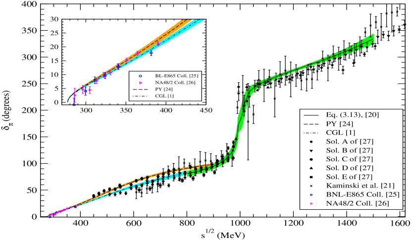
Figure 1: S-wave $I=0$ $\pi\pi$ phase shift, $\delta_{\pi}(s)$. Experimental data are from refs.[21, 25, 26, 27].

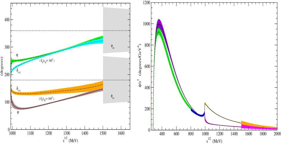
Figure 2: Left panel: Strong phase $\varphi(s)$, eigenvalue phase $\delta_{(+)}(s)$ and asymptotic phase $\phi_{as}(s)$. Right panel: Integrand of $\langle r^{2}\rangle_{s}^{\pi}$ in eq.(3.12) for parameterization I (dashed line) and II (solid line). For more details see the text. Notice that the uncertainty due to $\phi_{as}(s)$ is much reduced in the integrand.

Because of Watson final state theorem the phase $\phi(s)$ in eq.(2.1) is given by $\delta_{\pi}(s)$ below the $K\bar{K}$ threshold, neglecting inelasticity due to $4\pi$ or $6\pi$ states as indicated by experiments [20]. The situation above the $K\bar{K}$ threshold is more involved. Let us recall that

$$t_{\pi\pi}=(\eta\,e^{2i\delta_{\pi}}-1)/2i~{},$$ (2.4)

with $0\leq\eta\leq 1$ and the inelasticity is given by $1-\eta^{2}$, with $\eta$ the elasticity coefficient. We denote by $\varphi(s)$ the phase of $t_{\pi\pi}$, required to be continuous (below $4m_{K}^{2}$ it is given by $\delta_{\pi}(s)$). By continuity, close enough to the $K\bar{K}$ threshold and above it, $\eta\to 1$ and then we are in the same situation as in the elastic case. As a result, because of the Watson final state theorem and continuity, the phase $\phi(s)$ must still be given by $\varphi(s)$. For $\delta_{\pi}(s_{K})<\pi$, $s_{K}=4m_{K}^{2}$, $\varphi(s)$ does not follow the increasing trend with energy of $\delta_{\pi}(s)$ but drops as a result of eq.(2.4), see fig.2 for $\delta_{\pi}(s_{K})<\pi$. This is easily seen by writing explicitely the real and imaginary parts of $t_{\pi\pi}$ in eq.(2.4),

$$t_{\pi\pi}=\frac{1}{2}\eta\sin 2\delta_{\pi}+\frac{i}{2}(1-\eta\cos 2\delta_{\pi})~{}.$$ (2.5)

The imaginary part is always positive ($\eta<1$ above the $K\bar{K}$ threshold and 1.1 GeV [20]) while the real part is negative for $\delta_{\pi}<\pi$, but in an interval of just a few MeV the real part turns positive as soon as $\delta_{\pi}>\pi$, fig.1. As a result, $\varphi(s)$ passes quickly from values below but close to $\pi$ to the interval $[0,\pi/2]$. This rapid motion of $\phi(s)$ gives rise to a pronounced minimum of $|\Gamma_{\pi}(t)|$ at this energy, as indicated in ref.[13] and shown in fig.3. The drop in $\phi(s)$ becomes more and more dramatic as $\delta_{\pi}(s_{K})\to\pi^{-}$ (with the superscript $+(-)$ indicating that the limit is approached from values above(below), respectively); and in this limit, $\phi(s_{k})=\varphi(s_{K})$ is discontinuous at $s_{K}$. This is easily understood from eq.(2.5). Let us call $s_{1}$ the point at which $\delta_{\pi}(s_{1})=\pi$ with $s_{1}>s_{K}$. Close and above $s_{1}$, $\varphi(s)\in[0,\pi/2]$, for the reasons explained above, and $\varphi(s)$ has decreased very rapidly from almost $\pi$ at the $K\bar{K}$ threshold to values below $\pi/2$ just after $s_{1}$. Then, in the limit $s_{1}\to s_{K}^{+}$ one has $\phi(s_{K}^{-})=\varphi(s_{K}^{-})=\pi$ on the left, while on the right $\phi(s_{K}^{+})=\varphi(s_{K}^{+})<\pi/2$. As a result $\varphi(s)$ is discontinuous at $s=s_{K}$. We stress that this discontinuity of $\varphi(s)$ at $s_{K}$ when $\delta_{\pi}(s_{K})\to\pi^{-}$ applies rigorously to $\phi(s_{K})$ as well since $\eta(s_{K})=1$. This discontinuity at $s=s_{K}$ implies also that the integrand in the Omnès representation for $\Gamma_{\pi}(t)$ develops a logarithmic singularity as,

$$\frac{\phi(s_{K}^{-})-\phi(s_{K}^{+})}{\pi}\log\frac{\delta}{s_{K}}~{},$$ (2.6)

with $\delta\to 0^{+}$. When exponentiating this result one has a zero for $\Gamma_{\pi}(s_{K})$ as $(\delta/s_{K})^{\nu}$, $\nu=(\phi(s_{K}^{-})-\phi(s_{K}^{+}))/\pi>0$ and $\delta\to 0^{+}$. This zero is a necessary consequence when evolving continuously from $\delta_{\pi}(s_{K})<\pi$ to $\delta_{\pi}(s_{K})>\pi$. This in turn implies rigorously that in the Omnès representation of $\Gamma_{\pi}(t)$, eq.(2.1), $P(t)$ must be a polynomial of first degree for those cases with $\delta_{\pi}(s_{K})\geq\pi$,

$$P(t)=\Gamma_{\pi}(0)\frac{s_{1}-t}{s_{1}}~{},$$ (2.7)

with $s_{1}$ the position of the zero. Notice that the degree of the polynomial $P(t)$ is discrete and thus by continuity it cannot change unless a singularity develops. This is the case when $\delta_{\pi}(s_{K})=\pi$, changing the degree from 0 to 1. Hence, if $\delta_{\pi}(s_{K})\geq\pi$ for a given $t_{\pi\pi}$, instead of eqs.(2.2) and (2.3) one must then consider,

$$\Gamma_{\pi}(t)=\Gamma_{\pi}(0)\frac{s_{1}-t}{s_{1}}\exp\left[\frac{t}{\pi}\int_{4m_{\pi}^{2}}^{\infty}\frac{\phi(s)}{s(s-t)}ds\right]~{},$$ (2.8)

and

$$\langle r^{2}\rangle_{s}^{\pi}=-\frac{6}{s_{1}}+\frac{6}{\pi}\int_{4m_{\pi}^{2}}^{\infty}\frac{\phi(s)}{s^{2}}ds~{}.$$ (2.9)

For those $t_{\pi\pi}$ for which $\delta_{\pi}(s_{K})>\pi$ then $\varphi(s)$ follows $\delta_{\pi}(s)$ just after the $K\bar{K}$ threshold and there is no drop, as emphasized in ref.[11], see fig.2.

Summarizing, we have shown that $\Gamma_{\pi}(t)$ has a zero at $s_{1}$ when $\delta_{\pi}(s_{K})\geq\pi$ as a consequence of the assumption that $\phi(s)$ follows $\varphi(s)$ above the $K\bar{K}$ threshold, along the lines of ref.[11], and by imposing continuity in $\Gamma_{\pi}(t)$ under small changes in $\delta_{\pi}(s_{K})\simeq\pi$. As a result eqs.(2.8) and (2.9) should be used in the latter case, instead of eqs.(2.2) and (2.3), valid for $\delta_{\pi}(s_{K})<\pi$. This solution was overlooked in refs.[10, 11, 12]. We show in appendix A why the previous discussion on the zero of $\Gamma_{\pi}(t)$ for $\delta_{\pi}(s_{K})\geq\pi$ at $s_{1}$ cannot be applied to all pion scalar form factors, in particular to the strange one.

Figure 3: $|\Gamma_{\pi}(t)/\Gamma_{\pi}(0)|$ from eq.(2.2) with $\delta_{\pi}(s_{K})<\pi$, dashed-line, and $\delta_{\pi}(s_{K})>\pi$, dashed-dotted line. The solid line corresponds to use eq.(2.8) for the latter case. For this figure we have used parameterization II (defined in section 3) with $\alpha_{1}=2.28$ (dashed line) and 2.20 (dashed-dotted and solid lines). The dashed-double-dotted line is the scalar form factor of ref.[8] that has $\delta_{\pi}(s_{K})>\pi$.

If eq.(2.2) were used for those $t_{\pi\pi}$ with $\delta_{\pi}(s_{K})\geq\pi$ then a strong maximum of $|\Gamma_{\pi}(t)|$ would be obtained around the $K\bar{K}$ threshold, instead of the aforementioned zero or the minimum of refs.[4, 6], as shown in fig.3 by the dashed-dotted line. That is also shown in fig.10 of ref.[22] or fig.2 of [13]. This is the situation for the $\Gamma_{\pi}(t)$ of refs.[10, 11], and it is the reason why $\langle r^{2}\rangle_{s}^{\pi}$ obtained there is much larger than that of refs.[4, 1, 6]. That is, Ynduráin uses eqs.(2.2), (2.3) for $\delta_{\pi}(s_{K})\geq\pi$, instead of eqs.(2.8), (2.9) (solid line in fig.3). The unique and important role played by $\delta_{\pi}(s_{K})$ (for elastic $t_{\pi\pi}$ below the $K\bar{K}$ threshold) is perfectly recognised in ref.[11]. However, in this reference the astonishing conclusion that $\Gamma_{\pi}(t)$ has two radically different behaviours under tiny variations of $t_{\pi\pi}$ was sustained. These variations are enough to pass from $\delta_{\pi}(s_{K})<\pi$ to $\delta_{\pi}(s_{K})\geq\pi$ [10], while the $T-$ or $S-$matrix are fully continuous. Because of this instability of the solution of refs.[10, 11] under tiny changes of $\delta_{\pi}(s)$, we consider ours, that produces continuous $\Gamma_{\pi}(t)$, to be certainly preferred. We also stress that our solutions, either for $\delta_{\pi}(s_{K})\geq\pi$ and $\delta_{\pi}(s_{K})<\pi$, are the ones that agree with those obtained by solving the Muskhelishvili-Omnès equations [4, 1, 6] and Unitary $\chi$PT [8].

Let us now show how to fix $s_{1}$ in terms of the knowledge of $\delta_{\pi}(s)$ with $\delta_{\pi}(s_{K})\geq\pi$. For this purpose let us perform a dispersion relation of $\Gamma_{\pi}(t)$ with two subtractions,

$$\Gamma_{\pi}(t)=\Gamma_{\pi}(0)+\frac{1}{6}\langle r^{2}\rangle_{s}^{\pi}t+\frac{t^{2}}{\pi}\int_{4m_{\pi}^{2}}^{\infty}\frac{\hbox{Im}\Gamma_{\pi}(s)}{s^{2}(s-t)}ds~{},$$ (2.10)

From asymptotic QCD [23] one expects that the scalar form factor vanishes at infinity [10, 12], then the dispersion integral in eq.(2.10) should converge rather fast. Eq.(2.10) is useful because it tells us that the only point around 1 GeV where there can be a zero in $\Gamma_{\pi}(t)$ is at the energy $s_{1}$ for which the imaginary part of $\Gamma_{\pi}(t)$ vanishes. Otherwise, the integral in the right hand side of eq.(2.10) picks up an imaginary part and there is no way to cancel it as $\Gamma_{\pi}(0)$, $\langle r^{2}\rangle_{s}^{\pi}$ and $t$ are all real. Since $|\hbox{Im}\Gamma_{\pi}(t)|=|\Gamma_{\pi}(t)\,\sin\delta_{\pi}(t)|$ for $t\leq s_{K}$, it certainly vanishes at the point $s_{1}$ where $\delta_{\pi}(s_{1})=\pi$. As there is only one zero at such energies, this determines $s_{1}$ exactly in terms of the given parameterization for $\delta_{\pi}(s)$.

One could argue against the argument just given to determine $s_{1}$ that this energy could be complex. However, this would imply two zeroes at $s_{1}$ and $s_{1}^{*}$, and then the degree of $P(t)$ would be two instead of one. Notice that the degree of the polynomial $P(t)$ is discrete and thus, by softness in the continuous parameters of the $T-$matrix, its value should stay at 1 for some open domain in the parameters with $\delta_{\pi}(s_{K})>\pi$ until a discontinuity develops. Physically, the presence of two zeroes would in turn require that $\phi(s)\to 3\pi$ so as to guarantee that $\Gamma_{\pi}(t)$ still vanishes as $-1/t$, as required by asymptotic QCD [23, 10]. This value for the asymptotic phase seems to be rather unrealistic as $\varphi(s)$ only reaches $2\pi$ at already quite high energy values, as shown in fig.2.

3 Results

Our main result from the previous section is the sum rule to determine $\langle r^{2}\rangle_{s}^{\pi}$,

$$\langle r^{2}\rangle_{s}^{\pi}=-\frac{6}{s_{1}}\theta(\delta_{\pi}(s_{K})-\pi)+\frac{6}{\pi}\int_{4m_{\pi}^{2}}^{\infty}\frac{\phi(s)}{s^{2}}ds~{},$$ (3.11)

where $\theta(x)=0$ for $x<0$ and 1 for $x\geq 0$. We split $\langle r^{2}\rangle_{s}^{\pi}$ in two parts:

$$\langle r^{2}\rangle_{s}^{\pi} = Q_{H}+Q_{A}~{},$$

$$Q_{H} = -\frac{6}{s_{1}}\theta(\delta_{\pi}(s_{K})-\pi)+\frac{6}{\pi}\int_{4m_{\pi}^{2}}^{s_{H}}\frac{\phi(s)}{s^{2}}ds~{},$$

$$Q_{A} = \frac{6}{\pi}\int_{s_{H}}^{\infty}\frac{\phi(s)}{s^{2}}~{},$$ (3.12)

with $s_{H}=2.25$ GeV². Reasons for fixing $s_{H}$ to this value are given below.

The main issue in the application of eq.(3.11) is to determine $\phi(s)$ in the integrand. Below the $K\bar{K}$ threshold and neglecting inelasticity, one has that $\phi(s)=\delta_{\pi}(s)$, $4m_{\pi}^{2}\leq s\leq 4m_{K}^{2}$. This follows because of the Watson final state theorem, continuity and the equality $\phi(4m_{\pi}^{2})=\delta_{\pi}(4m_{\pi}^{2})=0$.

For practical applications we shall consider the S-wave I=0 $\pi\pi$ phase shifts given by the $K-$matrix parameterization of ref.[20] (from its energy dependent analysis of data from 0.6 GeV up to 1.9 GeV) and the parameterizations of ref.[1] (CGL) and ref.[24] (PY). The resulting $\delta_{\pi}(s)$ for all these parameterizations are shown in fig.1. We use CGL from $\pi\pi$ threshold up to 0.8 GeV, because this is the upper limit of its analysis, while PY is used up to 0.9 GeV, because at this energy it matches well inside the experimental errors with the data of [20]. The $K-$matrix of ref.[20] is used for energies above 0.8 GeV, when using CGL below this energy (parameterization I), and above 0.9 GeV, when using PY for lower energies (parameterization II). We take the parameterizations CGL and PY as their difference below 0.8 GeV accounts well for the experimental uncertainties in $\delta_{\pi}$, see fig.1, and they satisfy constraints from $\chi PT$ (the former) and dispersion relations (both). The reason why we skip to use the parameterization of ref.[20] for lower energies is because one should be there as precise as possible since this region gives the largest contribution to $\langle r^{2}\rangle_{s}^{\pi}$, as it is evident from the right panel of fig.2. It happens that the $K-$matrix of [20], that fits data above 0.6 GeV, is not compatible with data from $K_{e4}$ decays [25, 26]. We show in the insert of fig.1 the comparison of the parameterizations CGL and PY with the $K_{e4}$ data of [25, 26]. We also show in the same figure the experimental points on $\delta_{\pi}$ from refs.[20, 21, 27]. Both refs.[20, 21] are compatible within errors, with some disagreement above 1.5 GeV. This disagreement does not affect our numerical results since above 1.5 GeV we do not rely on data.

The $K-$matrix of ref.[20] is given by,

$$K_{ij}(s)=\alpha_{i}\alpha_{j}/(x_{1}-s)+\beta_{i}\beta_{j}/(x_{2}-s)+\gamma_{ij}~{},$$ (3.13)

where

$$\begin{array}[]{lll}x_{1}^{1/2}=0.11\pm 0.15{}&x_{2}^{1/2}=1.19\pm 0.01&\\ \alpha_{1}=2.28\pm 0.08{}&\alpha_{2}=2.02\pm 0.11&\\ \beta_{1}=-1.00\pm 0.03{}&\beta_{2}=0.47\pm 0.05&\\ \gamma_{11}=2.86\pm 0.15{}&\gamma_{12}=1.85\pm 0.18{}&\gamma_{22}=1.00\pm 0.53~{},\end{array}$$ (3.14)

with units given in appropriate powers of GeV. In order to calculate the contribution from the phase shifts of this $K-$matrix we generate Monte-Carlo gaussian samples, taking into account the errors shown in eq.(3.14), and evaluate $Q_{H}$ according to eq.(3.12). The central value of $\delta_{\pi}(s_{K})$ for the $K-$matrix of ref.[20] is $3.05$, slightly below $\pi$. When generating Monte-Carlo gaussian samples according to eq.(3.14), there are cases with $\delta_{\pi}(s_{K})\geq\pi$, around $30\%$ of the samples. Note that for these cases one also has the contribution $-6/s_{1}$ in eq.(3.11).

The application of Watson final state theorem for $s>4m_{K}^{2}$ is not straightforward since inelastic channels are relevant. The first important one is the $K\bar{K}$ channel associated in turn with the appearance of the narrow $f_{0}(980)$ resonance, just on top of its threshold. This implies a sudden drop of the elasticity parameter $\eta$, but it again rapidly raises (the $f_{0}(980)$ resonance is narrow with a width around 30 MeV) and in the region $1.1^{2}\lesssim s\lesssim 1.5^{2}$ GeV² is compatible within errors with $\eta=1$ [20, 21]. For $\eta\simeq 1$, the Watson final state theorem would imply again that $\phi(s)=\varphi(s)$, but, as emphasized by [13], this equality only holds, in principle, modulo $\pi$. The reason advocated in ref.[13] is the presence of the region $s_{K}<s<1.1^{2}$ GeV² where inelasticity can be large, and then continuity arguments alone cannot be applied to guarantee the equality $\phi(s)\simeq\varphi(s)$ for $s\gtrsim 1.1^{2}$ GeV². This argument has been proved in ref.[11] to be quite irrelevant in the present case. In order to show this a diagonalization of the $\pi\pi$ and $K\bar{K}$ $S-$matrix is done. These channels are the relevant ones when $\eta$ is clearly different from 1, between 1 and 1.1 GeV. Above that energy one also has the opening of the $\eta\eta$ channel and the increasing role of multipion states.

We reproduce here the arguments of ref.[11], but deliver expressions directly in terms of the phase shifts and elasticity parameter, instead of $K-$matrix parameters as done in ref.[11]. For two channel scattering, because of unitarity, the $T-$matrix can be written as:

$$T=\left(\begin{array}[]{ll}\frac{1}{2i}(\eta e^{2i\delta_{\pi}}-1)&\frac{1}{2}\sqrt{1-\eta^{2}}e^{i(\delta_{\pi}+\delta_{K})}\\ \frac{1}{2}\sqrt{1-\eta^{2}}e^{i(\delta_{\pi}+\delta_{K})}&\frac{1}{2i}(\eta e^{2i\delta_{K}}-1)\end{array}\right)~{},$$ (3.15)

with $\delta_{K}$ the elastic S-wave I=0 $K\bar{K}$ phase shift. In terms of the $T$-matrix the S-wave I=0 $S-$matrix is given by,

$$S=I+2iT~{},$$ (3.16)

satisfying $SS^{\dagger}=S^{\dagger}S=I$. The $T$-matrix can also be written as

$$T=Q^{1/2}\left(K^{-1}-iQ\right)^{-1}Q^{1/2}~{},$$ (3.17)

where the $K-$matrix is real and symmetric along the real axis for $s\geq 4m_{\pi}^{2}$ and $Q=diag(q_{\pi},q_{K})$, with $q_{\pi}(q_{K})$ the center of mass momentum of pions(kaons). This allows one to diagonalize $K$ with a real orthogonal matrix $C$, and hence both the $T-$ and $S-$matrices are also diagonalized with the same matrix. Writing,

$$C=\left(\begin{array}[]{cc}\cos\theta&\sin\theta\\ -\sin\theta&\cos\theta\end{array}\right)~{},$$ (3.18)

one has

$$\cos\theta = \frac{\left[(1-\eta^{2})/2\right]^{1/2}}{\left[1-\eta^{2}\cos^{2}\Delta-\eta|\sin\Delta|\sqrt{1-\eta^{2}\cos^{2}\Delta}\right]^{1/2}}~{},$$

$$\sin\theta = -\frac{\sin\Delta}{\sqrt{2}}\frac{\eta-\sqrt{1+(1-\eta^{2})\cot^{2}\Delta}}{\left[1-\eta^{2}\cos^{2}\Delta-\eta|\sin\Delta|\sqrt{1-\eta^{2}\cos^{2}\Delta}\right]^{1/2}}~{},$$ (3.19)

with $\Delta=\delta_{K}-\delta_{\pi}$. On the other hand, the eigenvalues of the $S-$matrix are given by,

$$e^{2i\delta_{(+)}} = S_{11}\frac{1+e^{2i\Delta}}{2}\left[1-\frac{i}{\eta}\tan\Delta\,\sqrt{1+(1-\eta^{2})\cot^{2}\Delta}\right]$$ (3.20)

$$e^{2i\delta_{(-)}} = S_{22}\frac{1+e^{-2i\Delta}}{2}\left[1+\frac{i}{\eta}\tan\Delta\,\sqrt{1+(1-\eta^{2})\cot^{2}\Delta}\right]~{}.$$ (3.21)

The eigenvalue phase $\delta_{(+)}$ satisfies $\delta_{(+)}(s_{K})=\delta_{\pi}(s_{K})$. The expressions above for $\exp 2i\delta_{(+)}$ and $\exp 2i\delta_{(-)}$ interchange between each other when $\tan\Delta$ crosses zero and simultaneously the sign in the right hand side of eq.(3.19) for $\sin\theta$ changes. This diagonalization allows to disentangle two elastic scattering channels. The scalar form factors attached to every of these channels, $\Gamma^{\prime}_{1}$ and $\Gamma^{\prime}_{2}$, will satisfy the Watson final state theorem in the whole energy range and then one has,

$$\Gamma^{\prime} \equiv \left(\begin{array}[]{c}\Gamma^{\prime}_{1}\\ \Gamma^{\prime}_{2}\end{array}\right)=C^{T}Q^{1/2}\Gamma=C^{T}Q^{1/2}\left(\begin{array}[]{c}\Gamma_{\pi}\\ \Gamma_{K}\end{array}\right)~{},$$ (3.26)

$$\Gamma_{\pi} = q^{-1/2}_{\pi}\left(\lambda\cos\theta\,|\Gamma_{1}^{\prime}|e^{i\delta_{(+)}}\pm\sin\theta\,|\Gamma_{2}^{\prime}|e^{i\delta_{(-)}}\right)~{},$$

$$\Gamma_{K} = q_{K}^{-1/2}\left(\pm\cos\theta\,|\Gamma_{2}^{\prime}|e^{i\delta_{(-)}}-\lambda\sin\theta\,|\Gamma_{1}^{\prime}|e^{i\delta_{(+)}}\right)~{}.$$ (3.27)

The $\pm$ in front of $|\Gamma^{\prime}_{2}|$ is due to the fact that $\Gamma^{\prime}_{2}=0$ at $s_{K}$, as follows from its definition in the equation above. Since Watson final state theorem only fixes the phase of $\Gamma^{\prime}_{2}$ up to modulo $\pi$, and the phase is not defined in the zero, we cannot fix the sign in front at this stage. Next, $\Gamma^{\prime}_{1}$ has a zero at $s_{1}$ when $\delta_{\pi}(s_{K})\geq\pi$. For this case, $-|\Gamma_{1}^{\prime}|$ must appear in the previous equation, so as to guarantee continuity of its ascribed phase, and this is why $\lambda=(-1)^{\theta(\delta_{\pi}(s_{K})-\pi)}$.

Now, when $\eta\to 1$ then $\sin\theta\to 0$ as $\sqrt{(1-\eta)/2}$ and $\phi(s)$ is then the eigenvalue phase $\delta_{(+)}$. This eigenvalue phase can be calculated given the $T-$matrix. For those $T-$matrices employed here, and those of refs.[10, 11, 4, 13], $\delta_{(+)}(s)$ follows rather closely $\varphi(s)$ in the whole energy range. This is shown in fig.2 and already discussed in detail in ref.[11]. In this way, one guarantees that $\phi(s)$ and $\varphi(s)$ do not differ between each other in an integer multiple of $\pi$ when $\eta\simeq 1$, $1.1^{2}\lesssim s\lesssim 1.5^{2}$ GeV².

For the calculation of $Q_{H}$ in eq.(3.12) we shall equate $\phi(s)=\varphi(s)$ for $4m_{K}^{2}<s<1.5^{2}$ GeV². Denoting,

$$I_{H} = \frac{6}{\pi}\int_{4m_{\pi}^{2}}^{s_{H}}\frac{\varphi(s)}{s^{2}}=I_{1}+I_{2}+I_{3}~{},$$

$$I_{1} = \frac{6}{\pi}\int_{4m_{\pi}^{2}}^{s_{K}}\frac{\varphi(s)}{s^{2}}ds~{},$$

$$I_{2} = \frac{6}{\pi}\int_{s_{K}}^{1.1^{2}}\frac{\varphi(s)}{s^{2}}ds~{},$$

$$I_{3} = \frac{6}{\pi}\int_{1.1^{2}}^{s_{H}}\frac{\varphi(s)}{s^{2}}ds~{},$$ (3.28)

then

$$Q_{H}\simeq I_{H}-\frac{6}{s_{1}}\theta(\delta_{\pi}(s_{K})-\pi)~{}.$$ (3.29)

Now, eq.(3.27) can also be used to estimate the error of approximating $\phi(s)$ by $\varphi(s)$ in the range $4m_{K}^{2}<s<1.5^{2}$ GeV² to calculate $I_{2}$ and $I_{3}$ as done in eq.(3.28). We could have also used $\delta_{(+)}(s)$ in eq.(3.28). However, notice that when $\eta\lesssim 1$ then $\varphi(s)\simeq\delta_{(+)}(s)$ and when inelasticity could be substantial the difference between $\delta_{(+)}(s)$ and $\varphi(s)$ is well taken into account in the error analysis that follows. Remarkably, consistency of our approach also requires $\phi(s)$ to be closer to $\varphi(s)$ than to $\delta_{(+)}(s)$. The reason is that $\varphi(s)$ for $\delta_{\pi}(s_{K})\geq\pi$ is in very good approximation the $\varphi(s)$ for $\delta_{\pi}(s_{K})<\pi$ plus $\pi$, this is clear from fig.2. This difference is $precisely$ the required one in order to have the same value for $\langle r^{2}\rangle_{s}^{\pi}$ either for $\delta_{\pi}(s_{K})<\pi$ or $\delta_{\pi}(s_{K})\geq\pi$ from eq.(3.11). However, the difference for $\delta_{(+)}(s)$ between $\delta_{\pi}(s_{K})<\pi$ and $\delta_{\pi}(s_{K})\geq\pi$ is smaller than $\pi$. Indeed, we note that $\phi(s)$ follows closer $\varphi(s)$ than $\delta_{(+)}(s)$ for the explicit form factors of refs.[8, 4].

Let us consider first the range $1.1^{2}<s<1.5^{2}$ GeV² where from experiment [20] $\eta\simeq 1$ within errors. With $\epsilon=\pm\tan\theta|\Gamma_{2}^{\prime}/\Gamma_{1}^{\prime}|$ and $\rho=\delta_{(-)}-\delta_{(+)}$, eq.(3.27) allows us to write,

$$\Gamma_{\pi}=\lambda\cos\theta\,|\Gamma_{1}^{\prime}|e^{i\delta_{(+)}}(1+\epsilon\cos\rho)\left(1+i\frac{\epsilon\sin\rho}{1+\epsilon\cos\rho}\right)~{}.$$ (3.30)

When $\eta\to 1$ then $\epsilon\to 0$, according to the expansion,

$$\tan\theta=\frac{\sqrt{(1-\eta)/2}}{\sin\Delta}\left[1-\frac{1+3\cos 2\Delta}{8\sin^{2}\Delta}(1-\eta)\right]+{\cal O}\left((1-\eta)^{5/2}\right)~{}.$$ (3.31)

Rewriting,

$$1+i\frac{\epsilon\sin\rho}{1+\epsilon\cos\rho}=\exp\left(i\frac{\epsilon\sin\rho}{1+\epsilon\cos\rho}\right)+{\cal O}(\epsilon^{2})~{},$$ (3.32)

which from eqs.(3.30) and (3.32) implies a shift in $\delta_{(+)}$ because of inelasticity effects,

$$\delta_{(+)}\to\delta_{(+)}+\frac{\epsilon\sin\rho}{1+\epsilon\cos\rho}~{}.$$ (3.33)

Using $\eta=0.8$ in the range $1.1^{2}\lesssim s\lesssim 1.5^{2}$ GeV, $\eta\simeq 1$ from the energy dependent analysis of ref.[20] given by the $K-$matrix of eq.(3.13), one ends with $\epsilon\simeq 0.3$. Taking into account that $\delta_{(+)}$ is larger than $\gtrsim 3\pi/2$ for $\delta_{\pi}(s_{K})\geq\pi$ (in this case $\delta_{(+)}\simeq\delta_{\pi}$), and around $3\pi/4$ for $\delta_{\pi}(s_{K})<\pi$, see fig.2, one ends with relative corrections to $\delta_{(+)}$ around $6\%$ for the former case and $13\%$ for the latter. Although the $K-$matrix of ref.[20], eq.(3.13), is given up to 1.9 GeV, one should be aware that to take only the two channels $\pi\pi$ and $K\bar{K}$ in the whole energy range is an oversimplification, particularly above 1.2 GeV. Because of this we finally double the previous estimate. Hence $I_{3}$ is calculated with a relative error of $12\%$ for $\delta_{\pi}(s_{K})\geq\pi$ and $25\%$ for $\delta_{\pi}(s_{K})<\pi$.

In the narrow region between $s_{K}<s<1.1^{2}$ GeV², $\eta$ can be rather different from 1, due to the $f_{0}(980)$ that couples very strongly to the just open $K\bar{K}$ channel. However, from the direct measurements of $\pi\pi\to K\bar{K}$ [29], where $1-\eta^{2}$ is directly measured, one has a better way to determine $\eta$ than from $\pi\pi$ scattering [20, 21]. It results from the former experiments, as shown also by explicit calculations [30, 31, 32], that $\eta$ is not so small as indicated in $\pi\pi$ experiments [20], and one has $\eta\simeq 0.6-0.7$ for its minimum value. Employing $\eta=0.6$ in eq.(3.33) then $\epsilon\simeq 0.5$. Taking $\delta_{(+)}$ around $\pi/2$ when $\delta_{\pi}(s_{K})<\pi$ this implies a relative error of 30$\%$. For $\delta_{\pi}(s_{K})\geq\pi$ one has instead $\delta_{(+)}\gtrsim\pi$, and a $15\%$ of estimated error. Regarding the ratio of the moduli of form factors entering in $\epsilon$ we expect it to be $\lesssim 1$ (see appendix A). Therefore, our error in the evaluation of $I_{2}$ is estimated to be $30\%$ and $15\%$ for the cases $\delta_{\pi}(s_{K})<\pi$ and $\delta_{\pi}(s_{K})\geq\pi$, respectively.

As a result of the discussion following eq.(3.29), we consider that the error estimates done for $I_{2}$ and $I_{3}$ in the case $\delta_{\pi}(s_{K})<\pi$ are too conservative and that the relative errors given for $\delta_{\pi}(s_{K})>\pi$ are more realistic. Nonetheless, since the absolute errors that one obtains for $I_{2}$ and $I_{3}$ are the same in both cases (because $I_{2}$ and $I_{3}$ for $\delta_{\pi}(s_{K})<\pi$ are around a factor 2 smaller than those for $\delta_{\pi}(s_{K})\geq\pi$) we keep the errors as given above. To the previous errors for $I_{2}$ and $I_{3}$ due to inelasticity, we also add in quadrature the noise in the calculation of $Q_{H}$ due to the error in $t_{\pi\pi}$ from the uncertainties in the parameters of the $K-$matrix eqs.(3.13), (3.14), and those in the parameterizations CGL and PY.

We finally employ for $s>2.25$ GeV² the knowledge of the asymptotic phase of the pion scalar form factor in order to evaluate $Q_{A}$ in eq.(3.12). The function $\phi(s)$ is determined so as to match with the asymptotic behaviour of $\Gamma_{\pi}(t)$ as $-1/t$ from QCD. The Omnès representation of the scalar form factor, eqs.(2.2) and (2.8), tends to $t^{-q/\pi}$ and $t^{-q/\pi+1}$ for $t\to\infty$, respectively. Here, $q$ is the asymptotic value of the phase $\phi(s)$ when $s\to\infty$. Hence, for $\delta_{\pi}(s_{K})<\pi$ the function $\phi(s)$ is then required to tend to $\pi$ while for $\delta_{\pi}(s_{K})\geq\pi$ the asymptotic value should be $2\pi$. The way $\phi(s)$ is predicted to approach the limiting value is somewhat ambiguous [11, 12],

$$\phi_{as}(s)\simeq\pi\left(n\pm\frac{2d_{m}}{\log(s/\Lambda^{2})}\right)~{}.$$ (3.34)

In this equation, $2d_{m}=24/(33-2n_{f})\simeq 1$, $\Lambda^{2}$ is the QCD scale parameter and $n=1,~{}2$ for $\delta_{\pi}(4m_{K}^{2})<\pi,~{}\geq\pi$, respectively. The case $n=2$ was not discussed in refs.[10, 11, 12, 13, 14] for the form factor given in eq.(1.1). There is as well a controversy between [14] and [12] regarding the $\pm$ sign in eq.(3.34). If leading twist contributions dominate [11, 12] then the limiting value is reached from above and one has the plus sign, while if twist three contributions are the dominant ones [14] the minus sign has to be considered [12]. In the left panel of fig.2 we show with the wide bands the values of $\phi(s)_{as}$ for $s>2.25$ GeV² from eq.(3.34), considering both signs, for $n=1$ ($\delta_{\pi}(s_{K})<\pi$) and $2$ ($\delta_{\pi}(s_{K})\geq\pi$). We see in the figure that above $1.4-1.5$ GeV ($1.96-2.25$ GeV²) both $\varphi(s)$ and $\phi(s)_{as}$ phases match and this is why we take $s_{H}=2.25$ GeV² in eq.(3.11), similarly as done in refs.[10, 11]. In this way, we also avoid to enter into hadronic details in a region where $\eta<1$ with the onset of the $f_{0}(1500)$ resonance. The present uncertainty whether the $+$ or $-$ sign holds in eq.(3.34) is taken as a source of error in evaluating $Q_{A}$. The other source of uncertainty comes from the value taken for $\Lambda^{2}$, $0.1<\Lambda^{2}<0.35$ GeV², as suggested in ref.[10]. From fig.2 it is clear that our error estimate for $\phi_{as}(s)$ is very conservative and should account for uncertainties due to the onset of inelasticity for energies above $1.4-1.5$ GeV and to the appearance of the $f_{0}(1500)$ resonance. In the right panel of fig.2 we show the integrand for $\langle r^{2}\rangle_{s}^{\pi}$, eq.(3.12), for parameterization I (dashed line) and II (solid line). Notice as the large uncertainty in $\phi_{as}(s)$ is much reduced in the integrand as it happens for the higher energy domain.

$\phi(s)$	I	I	II	II
$\delta_{\pi}(s_{K})$	$\geq\pi$	$<\pi$	$\geq\pi$	$<\pi$
$I_{1}$	$0.435\pm 0.013$	$0.435\pm 0.013$	$0.483\pm 0.013$	$0.483\pm 0.013$
$I_{2}$	$0.063\pm 0.010$	$0.020\pm 0.006$	$0.063\pm 0.010$	$0.020\pm 0.006$
$I_{3}$	$0.143\pm 0.017$	$0.053\pm 0.013$	$0.143\pm 0.017$	$0.053\pm 0.013$
$Q_{H}$	$0.403\pm 0.024$	$0.508\pm 0.019$	$0.452\pm 0.024$	$0.554\pm 0.019$
$Q_{A}$	$0.21\pm 0.03$	$0.10\pm 0.03$	$0.21\pm 0.03$	$0.10\pm 0.03$
$\langle r^{2}\rangle_{s}^{\pi}$	$0.61\pm 0.04$	$0.61\pm 0.04$	$0.66\pm 0.04$	$0.66\pm 0.04$

Table 1: Different contributions to $\langle r^{2}\rangle_{s}^{\pi}$ as defined in eqs.(3.12) and (3.28). All the units are $\textrm{fm}^{2}$. In the value for $\langle r^{2}\rangle_{s}^{\pi}$ the errors due to $I_{1}$, $I_{2}$, $I_{3}$ and $Q_{A}$ are added in quadrature.

In table 1 we show the values of $I_{1}$, $I_{2}$, $I_{3}$, $Q_{H}$, $Q_{A}$ and $\langle r^{2}\rangle_{s}^{\pi}$ for the parameterizations I and II and for the two cases $\delta_{\pi}(s_{K})\geq\pi$ and $\delta_{\pi}(s_{K})<\pi$. This table shows the disappearance of the disagreement between the cases $\delta_{\pi}(s_{K})\geq\pi$ and $\delta_{\pi}(s_{K})<\pi$ from the $\pi\pi$ and $K\bar{K}$ $T-$matrix of eq.(3.13), once the zero of $\Gamma_{\pi}(t)$ at $s_{1}<s_{K}$ is taken into account for the former case. This disagreement was the reason for the controversy between Ynduráin and ref.[13] regarding the value of $\langle r^{2}\rangle_{s}^{\pi}$. The fact that the parameterization II gives rise to a larger value of $\langle r^{2}\rangle_{s}^{\pi}$ than I is because PY follows the upper $\delta_{\pi}$ data below 0.9 GeV, while CGL follows lower ones, as shown in fig.1.

The different errors in table 1 are added in quadrature. The final value for $\langle r^{2}\rangle_{s}^{\pi}$ is the mean between those of parameterizations I and II and the error is taken such that it spans the interval of values in table 1 at the level of two sigmas. One ends with:

$$\langle r^{2}\rangle_{s}^{\pi}=0.63\pm 0.05~{}\hbox{fm}^{2}~{}.$$ (3.35)

The largest sources of error in $\langle r^{2}\rangle_{s}^{\pi}$ are the uncertainties in the experimental $\delta_{\pi}$ and in the asymptotic phase $\phi_{as}$. This is due to the fact that the former are enhanced because of its weight in the integrand, see fig.2, and the latter due to its large size.

Our number above and that of refs.[1, 4], $\langle r^{2}\rangle_{s}^{\pi}=0.61\pm 0.04$ fm², are then compatible. On the other hand, we have also evaluated $\langle r^{2}\rangle_{s}^{\pi}$ directly from the scalar form factor obtained with the dynamical approach of ref.[8] from Unitary $\chi$PT and we obtain $\langle r^{2}\rangle_{s}^{\pi}=0.64\pm 0.06$ fm², in perfect agreement with eq.(3.35). Notice that the scalar form factor of ref.[8] has $\delta_{\pi}(s_{K})>\pi$ and we have checked that it has a zero at $s_{1}$, as it should. This is shown in fig.3 by the dashed-double-dotted line. The value $\langle r^{2}\rangle_{s}^{\pi}=0.75\pm 0.07$ fm² from refs.[10, 11] is much larger than ours because the possibility of a zero at $s_{1}$ was not taking into account there and other solution was considered. This solution, however, has an unstable behaviour under the transition $\delta_{\pi}(s_{K})=\pi-0^{+}$ to $\delta_{\pi}(s_{K})=\pi+0^{+}$ and it cannot be connected continuously with the one for $\delta_{\pi}(s_{K})<\pi$. Our solution for $\Gamma_{\pi}(t)$ from Ynduráin’s method does not have this unstable behaviour and it is continuous under changes in the values of the parameters of the $K-$matrix, eqs.(3.13) and (3.14). This is why, from our results, it follows too that the interesting discussion of ref.[11], regarding whether $\delta_{\pi}(s_{K})<\pi$ or $\geq\pi$, is not any longer conclusive to explain the disagreement between the values of refs.[10, 11] and ref.[1] for $\langle r^{2}\rangle_{s}^{\pi}$.

We can also work out from our determination of $\langle r^{2}\rangle_{s}^{\pi}$, eq.(3.35), values for the ${\cal O}(p^{4})$ $SU(2)$ $\chi PT$ low energy constant $\bar{\ell}_{4}$. We take the two loop expression in $\chi PT$ for $\langle r^{2}\rangle_{s}^{\pi}$ [1],

$$\langle r^{2}\rangle_{s}^{\pi}=\frac{3}{8\pi^{2}f_{\pi}^{2}}\left\{\bar{\ell}_{4}-\frac{13}{12}+\xi\Delta_{r}\right\}~{},$$ (3.36)

where $f_{\pi}=92.4$ MeV is the pion decay constant, $\xi=(M_{\pi}/4\pi f_{\pi})^{2}$ and $M_{\pi}$ is the pion mass. First, at the one loop level calculation $\Delta_{r}=0$ and then one obtains,

$$\bar{\ell}_{4} = 4.7\pm 0.3~{}.$$ (3.37)

We now move to the determination of $\bar{\ell}_{4}$ based on the full two loop relation between $\langle r^{2}\rangle_{s}^{\pi}$ and $\bar{\ell}_{4}$. The expression for $\Delta_{r}$ can be found in Appendix C of ref.[1]. $\Delta_{r}$ is given in terms of one ${\cal O}(p^{6})$ $\chi PT$ counterterm, $\widetilde{r}_{S_{2}}$, and four ${\cal O}(p^{4})$ ones. Taking the values of all these parameters, but for $\bar{\ell}_{4}$, from ref.[1], and solving for $\bar{\ell}_{4}$, one arrives to

$$\bar{\ell}_{4} = 4.5\pm 0.3~{}.$$ (3.38)

This number is in good agreement with $\bar{\ell}_{4}=4.4\pm 0.2$ [1].

Ref.[12] also points out that one loop $\chi$PT fits to the S-, P- and D-wave scattering lengths and effective ranges give rise to much larger values for $\bar{\ell}_{2}$ and $\bar{\ell}_{4}$ than those of ref.[1]. For more details we refer to [12].

4 Conclusions

In this paper we have addressed the issue of the discrepancies between the values of the quadratic pion scalar radius of Leutwyler et al. [4, 13], $\langle r^{2}\rangle_{s}^{\pi}=0.61\pm 0.04$ fm², and Ynduráin’s papers [10, 11, 12], $\langle r^{2}\rangle=0.75\pm 0.07$ fm². One of the reasons of interest for having a precise determination of $\langle r^{2}\rangle_{s}^{\pi}$ is its contribution of a 10$\%$ to $a_{0}^{0}$ and $a_{0}^{2}$, calculated with a precision of $2\%$ in ref.[1]. The value taken for $\langle r^{2}\rangle_{s}^{\pi}$ is also important for determining the ${\cal O}(p^{4})$ $\chi$PT coupling $\bar{\ell}_{4}$.

From our study it follows that Ynduráin’s method to calculate $\langle r^{2}\rangle_{s}^{\pi}$ [10, 11], based on an Omnès representation of the pion scalar form factor, and that derived by solving the two(three) coupled channel Muskhelishvili-Omnès equations [4, 1, 6], are compatible. It is shown that the reason for the aforementioned discrepancy is the presence of a zero in $\Gamma_{\pi}(t)$ for those S-wave I=0 $T-$matrices with $\delta_{\pi}(s_{K})\geq\pi$ and elastic below the $K\bar{K}$ threshold, with $s_{K}=4m_{K}^{2}$. This zero was overlooked in refs.[10, 11], though, if one imposes continuity in the solution obtained under tiny changes of the $\pi\pi$ phase shifts employed, it is necessarily required by the approach followed there. Once this zero is taken into account the same value for $\langle r^{2}\rangle_{s}^{\pi}$ is obtained irrespectively of whether $\delta_{\pi}(s_{K})\geq\pi$ or $\delta_{\pi}(s_{K})<\pi$. Our final result is $\langle r^{2}\rangle_{s}^{\pi}=0.63\pm 0.05$ fm². The error estimated takes into account experimental uncertainty in the values of $\delta_{\pi}(s)$, inelasticity effects and present ignorance in the way the phase of the form factor approaches its asymptotic value $\pi$, as predicted from QCD. Employing our value for $\langle r^{2}\rangle_{s}^{\pi}$ we calculate $\bar{\ell}_{4}=4.5\pm 0.3$. The values $\langle r^{2}\rangle_{s}^{\pi}=0.61\pm 0.04$ fm² and $\bar{\ell}_{4}=4.5\pm 0.3$ of ref.[1] are then in good agreement with ours.

Appendices

Appendix A Coupled channel dynamics

We take $\pi\pi$ and $K\bar{K}$ coupled channels and denote by $F_{1}$ and $F_{2}$ their respective I=0 scalar form factors. Unitarity requires,

$$\hbox{Im}F_{i}=\sum_{j=1}^{2}F_{j}\rho_{j}\theta(t-s^{\prime}_{j})t_{ji}^{*}~{},$$ (A.1)

where $||t_{ij}||$ is the I=0 S-wave $T-$matrix, $s^{\prime}_{i}$ is the threshold energy square of channel $i$ and $\rho_{i}=q_{i}/8\pi\sqrt{s}$, with $q_{i}$ its center of mass three momentum.

A general solution to the previous equations is given by,

$$F=T\,G~{},~{}F=\left(\begin{array}[]{c}F_{1}\\ F_{2}\end{array}\right)~{},~{}G=\left(\begin{array}[]{c}G_{1}\\ G_{2}\end{array}\right)~{},$$ (A.2)

where the functions $G_{i}(t)$ do not have right hand cut. This equation is interesting as tells us that if pion dynamics dominate, $|G_{1}|>>|G_{2}|$, then $F_{1}\simeq G_{1}t_{11}$ and the form factor phase $\phi(s)$ follows $\varphi(s)$. As a result, like $t_{11}$, it has a zero at $s_{1}$ below the $K\bar{K}$ threshold for $\delta_{\pi}(s_{K})\geq\pi$, as shown in section 3. On the other hand, if kaon dynamics dominates, $|G_{2}|>>|G_{1}|$, then $F_{1}\simeq G_{2}t_{12}$ and $\phi(s)$ follows the phase of $t_{12}$, that above the $K\bar{K}$ threshold is clearly above $\pi$. This is why for the pion strange scalar form factor there is no zero at $s_{1}\lesssim s_{K}$ for $\delta_{\pi}(s_{K})\geq\pi$, indeed there is a maximum like that shown in fig.3 by the dashed-dotted line.

As in section 3 we now proceed to the diagnolization above the $K\bar{K}$ threshold of the renormalized $T-$matrix $T^{\prime}$,

$$T^{\prime}=\rho^{1/2}T\rho^{1/2}~{},~{}\rho=\left(\begin{array}[]{c}\rho_{1}^{1/2}\\ \rho_{2}^{1/2}\end{array}\right)~{},~{}\widetilde{T}=C^{T}T^{\prime}C=\left(\begin{array}[]{cc}\widetilde{t}_{11}&0\\ 0&\widetilde{t}_{22}\end{array}\right)~{},$$ (A.7)

$$\widetilde{t}_{11}=\sin\delta_{(+)}e^{i\delta_{(+)}}~{},~{}\widetilde{t}_{22}=\sin\delta_{(-)}e^{i\delta_{(-)}}~{}.$$ (A.8)

The corresponding diagonal form factors $F^{\prime}_{1}$ and $F^{\prime}_{2}$, collected in the vector $F^{\prime}$, are

$$F^{\prime} = C^{T}\rho^{1/2}F=\widetilde{T}C^{T}\rho^{-1/2}G=\left(\begin{array}[]{ll}\left\{\cos\theta\,\rho_{1}^{-1/2}G_{1}-\sin\theta\,\rho^{-1/2}_{2}G_{2}\right\}\widetilde{t}_{11}\\ \left\{\sin\theta\,\rho_{1}^{-1/2}G_{1}+\cos\theta\,\rho_{2}^{-1/2}G_{2}\right\}\widetilde{t}_{22}\end{array}\right)~{}.$$ (A.11)

The previous expressions allow to obtaining $F_{1}$ directly in terms of the eigenphases and with clean separation between pion, $G_{1}$, and kaon dynamics, $G_{2}$. From eq.(3.27) it follows that,

$$\begin{aligned} F_{1}=&\left\{\cos^{2}\theta\,\rho^{-1}G_{1}-\cos\theta\,\sin\theta\,\rho_{2}^{-1/2}\rho_{1}^{-1/2}G_{2}\right\}\widetilde{t}_{11}\\ +&\left\{\sin^{2}\theta\,\rho_{1}^{-1}G_{1}+\cos\theta\,\sin\theta\,\rho_{2}^{-1/2}\rho_{1}^{-1/2}G_{2}\right\}\widetilde{t}_{22}~{}.\end{aligned}$$ (A.12)

For $\delta_{\pi}(s_{K})\geq\pi$ typical values, somewhat above the $K\bar{K}$ threshold, are $e^{2i\delta_{(+)}}\simeq+i$, $e^{2i\delta_{(-)}}\simeq-i$ and $\sin\theta>0$. For dominance of $G_{1}$ one has $F_{1}/G_{1}\simeq\rho_{1}^{-1}(i+\cos 2\theta)/2$ while for dominance of $G_{2}$ the result is $F_{1}/G_{2}\simeq-\sin\theta\,\cos\theta\,\rho_{2}^{-1/2}\rho_{1}^{-1/2}<0$. The factors $G_{1,2}$ do not introduce any change in $\phi(s)$ with respect to its value before the opening of the $K\bar{K}$ threshold since they are smooth functions in $s$. In both cases the phase $\phi(s)$ is larger than $\pi$ and $F_{1}$ follows the upper trend of phases shown in fig.2 (note that in this case $\widetilde{t}_{11}$ is in the first quadrant though $\delta_{\pi}>\pi$). Now, doing the same exercise for $\delta_{\pi}(s_{K})<\pi$, one has the typical values $e^{2i\delta_{(+)}}\simeq-i$, $e^{2i\delta_{(-)}}\simeq+i$ and $\sin\theta<0$. For pion dominance then $F_{1}/G_{1}\simeq\rho_{1}^{-1}(i-\cos 2\theta)/2$ and for the kaon one $F_{1}/G_{2}\simeq+\sin\theta\cos\theta\rho_{2}^{-1/2}\rho_{1}^{-1/2}<0$. Thus, in the former case the phase is $\gtrsim\pi/2$, and follows the lower trend of phases of fig.2, while in the latter is $\gtrsim\pi$ and follows again the upper trend (this is the case of the strange scalar form factor).

The demonstration in section 3 that $\phi(s_{K})$ is discontinuous in the limit $\delta_{\pi}(s_{K})\to\pi^{-}$ by taking $s_{1}\to s_{K}^{+}$, cannot be applied in the case of kaon dominance (e.g. pion strange scalar form factor). From eq.(A.12) it follows that,

$$F_{1}(t)\simeq-\cos\theta\sin\theta\rho_{2}^{-1/2}\rho_{1}^{-1/2}G_{2}\left(\widetilde{t}_{11}-\widetilde{t}_{22}\right)~{}.$$ (A.13)

The point is that $\widetilde{t}_{22}$ for $t\geq s_{1}$ ($s_{1}\to s_{K}^{+}$) is of size comparable with that of $\widetilde{t}_{11}$ (both tend to zero) and the phase does not follow $\delta_{(+)}$. This is not the case for pion dominance because for $s_{1}\to s_{K}^{+}$ then $\sin^{2}\theta\to 0$, $F_{1}(t)\simeq\cos^{2}\theta\,\rho_{1}^{-1}G_{1}\widetilde{t}_{11}$, eq.(A.12), and $\phi(s)$ follows $\delta_{(+)}$.

From eq.(A.11) we can also write $|\Gamma^{\prime}_{2}/\Gamma^{\prime}_{2}|\simeq|\widetilde{t}_{11}\tan\theta/\widetilde{t}_{22}|$ for the case of pion dominance. Since typically $|\widetilde{t}_{11}/\widetilde{t}_{22}|\simeq 1$, as shown above for energies somewhat above the $K\bar{K}$ threshold, then $|\Gamma^{\prime}_{2}/\Gamma^{\prime}_{1}|\simeq|\tan\theta|<1$. This is why we consider that equating it to 1 in section 3 is a conservative estimate.

References

[1] G. Colangelo, J. Gasser and H. Leutwyler, Nucl. Phys. B603, 125 (2001).
[2]J. Gasser and H. Leutwyler, Phys. Lett. B125, 325 (1983).
[3]G. Colangelo and S. Dür, Eur. Phys. J. C33, 543 (2004).
[4] J. F. Donoghue, J. Gasser and H. Leutwyler, Nucl. Phys. B343, 341 (1990).
[5]B. Ananthanarayan, G. Colangelo, J. Gasser and H. Leutwyler, Phys. Rep.
353, 207 (2001).
[6]B. Moussallam, Eur. Phys. J. C14, 111 (2000).
[7]J. Gasser and U.-G. Meißner, Nucl. Phys. B357, 90 (1991).
[8]U. G. Meißner and J. A. Oller, Nucl. Phys. A679, 671 (2001).
[9]J. Bijnens, G. Colangelo and P. Talavera, JHEP 9805, 014 (1998).
[10]F. J. Ynduráin, Phys. Lett. B578, 99 (2004); (E)- B586, 439 (2004).
[11]F. J. Ynduráin, Phys. Lett. B612, 245 (2005).
[12]F. J. Ynduráin, arXiv:hep-ph/0510317.
[13]B. Ananthanarayan, I. Caprini, G. Colangelo, J. Gasser and H. Leutwyler, Phys.
Lett. B602, 218 (2004).
[14]I. Caprini, G. Colangelo and H. Leutwyler, Int. J. Mod. Phys. A21, 954 (2006).
[15]M. Jamin, J.A. Oller and A. Pich, JHEP 0402, 047 (2004);
Phys. Rev. D74, 074009 (2006).
[16]M. Jamin, J.A. Oller and A. Pich, Nucl. Phys. B 587, 331 (2000).
[17]J. Bijnens and P. Talavera, Nucl. Phys. B669, 341 (2003).
[18]O. P. Yushchenko et al., Phys. Lett. B581, 31 (2004).
[21] R. Kaminski, L. Lesniak and K. Rybicki, Z. Phys. C 74, 79 (1997).
[22] F. Guerrero and J. A. Oller, Nucl. Phys. B537, 459 (1999); (E)-. B602, 641 (2001).
[23] S. J. Brodsky and G. P. Lepage, Phys. Rev. D22, 2157 (1980).
[24]J. R. Peláez and F. J. Ynduráin, Phys. Rev. D68, 074005 (2003);
D71, 074016 (2005).
[25] S Pislak et al. [BNL-E865 Collaboration], Phys. Rev.
Lett. 87, 221801; Phys. Rev. D67, 072004 (2003).
[26] L. Masetti [NA48/2 Collaboration], arXiv:hep-ex/0610071.
[27] G. Grayer et al., Nucl. Phys. B 75 (1974) 189.
[28] W.-M. Yao et al., Journal of Physics G33, 1 (2006).
[29]W. Wetzel et al., Nucl. Phys. B115, 208 (1976); V. A.
Polychromatos et al., Phys. Rev. D19, 1317 (1979); D. Cohen et al.
Phys. Rev. D22, 2595 (1980); E. Etkin et al., Phys. Rev. D25, 1786 (1982).
[30]J. A. Oller and E. Oset, Nucl. Phys. A 620 (1997) 438
(E)-. A 652 (1999) 407].
[31] J. A. Oller and E. Oset, Phys. Rev. D 60 (1999) 074023.
[32]M. Albaladejo and J. A. Oller, forthcoming. Here the channel is included.