Filling-Factor-Dependent Magnetophonon Resonance in Graphene

Abstract

We describe a peculiar fine structure acquired by the in-plane optical phonon at the $\Gamma$-point in graphene when it is brought into resonance with one of the inter-Landau-level transitions in this material. The effect is most pronounced when this lattice mode (associated with the G-band in graphene Raman spectrum) is in resonance with inter-Landau-level transitions $0\Rightarrow+,1$ and $-,1\Rightarrow 0$, at a magnetic field $B_{0}\simeq 30$T. It can be used to measure the strength of the electron-phonon coupling directly, and its filling-factor dependence can be used experimentally to detect circularly polarized lattice vibrations.

In metals and semiconductors the spectra of phonons are renormalized by their interaction with electrons. Some of the best known examples include the Kohn anomaly kohn in the phonon dispersion, which originates from the excitation/de-excitation of electrons across the Fermi level upon the propagation of a phonon through the bulk of a metal and a shift in the longitudinal optical phonon frequency in heavily doped polar semiconductors mahan . However, despite the transparency of theoretical models the observation of such effects is often obscured by the difficulty to change the electron density in a material, whereas in semiconductor structures containing two-dimensional (2D) electrons the density of which can be varied, the influence of the latter on the phonon modes is weak due to a negligibly small volume fraction occupied by the electron gas. In this context, a unique opportunity arises in graphene-based field-effect transistors geim , where the density of carriers in an atomically thin film (monolayer novoselov1 ; zhang1 ; zhang2 or a bilayer geim2 ) can be continuously varied from 10¹³cm^-2 p-type to 10¹³cm^-2 n-type. Several Raman experiments have already been reported pisana ; yan where the variation of carrier density in graphene changes the optical phonon frequency, in agreement with theoretical expectations ando ; castroneto ; lazzeri .

When graphene is exposed to a quantizing magnetic field, its electronic spectrum quenches into discrete Landau levels (LLs) McClure . Then, the optical phonon energy in graphene may coincide with the energy of one of the inter-LL transitions, a condition known as magnetophonon resonance magnetophonon ; Nicholas . Recently, Ando has suggested AndoMP that in undoped graphene the magnetophonon resonance enhances the effect of the electron-phonon coupling on a spectrum of the in-plane optical phonons - the E_2g modes attributed to the G-band in the Raman spectra in Refs. ferrari ; gupta ; graf ; pisana ; yan . In this paper, we investigate a rich structure of the anti-crossing experienced by such lattice modes when a magnetic field makes their energy equal to the energy of one of the valley-antisymmetric interband magnetoexcitons magnetooptics . Most saliently, the difference between circular polarization of various inter-LL transitions sadowski ; Abergel makes the magnetophonon resonance distinguishable for lattice vibrations of different circular polarization, which makes the number of split lines in the fine structure acquired by a phonon and the value of splitting dependent on the electronic filling factor, $\nu$.

The in-plane optical phonons in graphene [relative displacement $\mathbf{u}=(u_{x},u_{y})$ of sublattices $A$ and $B$] have the energy $\omega\approx 0.2$eV at the $\Gamma$-point (in the center of the Brillouin zone). These phonons and their coupling to electrons can be described using the Hamiltonian ando ; castroneto ,

$$H_{\mathrm{ph}} = \sum_{\mu,\mathbf{q}}\omega b_{\mu,\mathbf{q}}^{\dagger}b_{\mu,\mathbf{q}}+g\sqrt{2M\omega}(\sigma_{x}u_{y}-\sigma_{y}u_{x}),$$ (1)

$$\mathbf{u}(\mathbf{r}) = \sum_{\mu,\mathbf{q}}\frac{1}{\sqrt{2N_{uc}M\omega}}\left(b_{\mu,\mathbf{q}}+b_{\mu,-\mathbf{q}}^{\dagger}\right)\mathbf{e}_{\mu,\mathbf{q}}e^{-i\mathbf{q}\cdot\mathbf{r}},$$

where $b_{\mu,\mathbf{q}}^{(\dagger)}$ are annihilation (creation) operators of a phonon with polarisation $\mathbf{e}_{\mu,\mathbf{q}}$, $M$ is the mass of a carbon atom, and $N_{uc}$ is the number of unit cells. Here and below, we use units $\hbar\equiv 1$. Also, we shall utilize a double degeneracy of the E_2g mode at the $\Gamma$-point (at $\mathbf{q}=0$) and describe the in-plane optical phonon in terms of a degenerate pair of circularly polarized modes, $u_{\circlearrowleft}=(u_{x}+iu_{y})/\sqrt{2}$ and $u_{\circlearrowright}=u_{\circlearrowleft}^{*}$. The constant $g$ in Eq. (1) characterizes the electron-phonon coupling footnote1 . This coupling has the form of the only invariant linear in $\mathbf{u}$ permitted by the symmetry group of the honeycomb crystal. It is constructed using Pauli matrices ${\mbox{\boldmath$\sigma$}}=(\sigma_{x},\sigma_{y})$ acting in the space of sublattice components of the Bloch functions, ${[}\phi_{\mathbf{K}_{+}A}$, $\phi_{\mathbf{K}_{+}B}]$ and $[\phi_{\mathbf{K}_{-}B}$, $\phi_{\mathbf{K}_{-}A}]$ which describe electron states in the valleys $\mathbf{K}_{\pm}$ (two opposite corners of the hexagonal Brillouin zone) and obey the Hamiltonian, in terms of the electron charge $-e<0$ footnote2 ,

$$H_{\mathrm{el}}=\xi v\mbox{\boldmath$\sigma$}\cdot\mathbf{p},~{}~{}\mathbf{\;p=}-i\mathbf{\nabla}+e\mathbf{A,\;}~{}~{}\partial_{x}A_{y}-\partial_{y}A_{x}=B.$$

Here, $\xi=\pm$ distinguishes between $\mathbf{K}_{\pm}$, and momentum $\mathbf{\mathbf{p}}$ is calculated with respect to the center of the corresponding valley. This Hamiltonian represents the dominant term of the next-neighbor tight-binding model of graphene wallace ; Dresselhaus ; AndoReview , and the electron-phonon coupling in Eq. (1) takes into account the change in the $A-B$ hopping elements due to the sublattice displacement symmetry .

In a perpendicular magnetic field, $H_{\mathrm{el}}$ determines McClure a spectrum of 4-fold (spin and valley) degenerate LLs, $\varepsilon_{n}^{\alpha=\pm}=\alpha\sqrt{2n}v\lambda_{B}^{-1}$ in the valence band ($\varepsilon_{n>0}^{-}$), conduction band ($\varepsilon_{n>0}^{+}$), and at zero energy ($\varepsilon_{0}=0$, exactly at the Dirac point in the electron spectrum), in terms of the magnetic length $\lambda_{B}=1/\sqrt{eB}$. Such a spectrum has been confirmed by recent quantum Hall effect measurements novoselov1 ; zhang1 ; zhang2 . In each of the two valleys, the LL basis is given by two-component states $\sqrt{\frac{1}{2}}[\sqrt{1+\delta_{n,0}}\phi_{n,m},i\xi\alpha(1-\delta_{n,0})\phi_{n-1,m}]$, where $\phi_{n,m}$ are the LL wave functions described by the quantum numbers $n$ and $m$, the latter being related to the guiding center degree of freedom. Here, we neglect the Zeeman effect, and simply take into account the two-fold spin degeneracy.

Figure 1: (a) Optical phonons are lattice vibrations with an out-off-phase oscillation of the two sublattices. (b) Interband electron-hole excitations coupling to phonon modes with different circular polarization.

Excitations of electrons between LLs can be described in terms of magnetoexcitons (see Fig. 1). Those relevant for the magnetophonon resonance are

$$\psi_{\circlearrowleft}^{\dagger}(n,\xi) = \frac{i\sqrt{1+\delta_{n,0}}}{\mathcal{N}_{n}^{\circlearrowleft}}\sum_{m}c_{+,n,m;\xi}^{\dagger}c_{-,(n+1),m;\xi},$$

$$\psi_{\circlearrowright}^{\dagger}(n,\xi) = \frac{i\sqrt{1+\delta_{n,0}}}{\mathcal{N}_{n}^{\circlearrowright}}\sum_{m}c_{+,(n+1),m;\xi}^{\dagger}c_{-,n,m;\xi},$$ (2)

where the index $\mathcal{A}=\circlearrowleft,\circlearrowright$ characterizes the angular momentum of the excitation and the operators $c_{\alpha,n,m;\xi}^{(\dagger)}$ annihilate (create) an electron in the state $\alpha,n,m$ in the valley $\mathbf{K}_{\xi}$. The normalization factors $\mathcal{N}_{n}^{\circlearrowleft}=[(1+\delta_{n,0})N_{B}(\bar{\nu}_{-,(n+1)}-\bar{\nu}_{+,n})]^{1/2}$ and $\mathcal{N}_{n}^{\circlearrowright}=[(1+\delta_{n,0})N_{B}(\bar{\nu}_{-,n}-\bar{\nu}_{+,(n+1)})]^{1/2}$ are used to ensure the bosonic commutation relations of the exciton operators, $[\psi_{\mathcal{A}}(n,\xi),\psi_{\mathcal{A}^{\prime}}^{\dagger}(n^{\prime},\xi^{\prime})]=\delta_{\mathcal{A},\mathcal{A}^{\prime}}\delta_{\xi,\xi^{\prime}}\delta_{n,n^{\prime}}$, where $N_{B}$ is the total number of states per LL in a sample, including the two-fold spin-degeneracy. These commutation relations are obtained within the mean-field approximation with $\langle c_{\alpha,n,m;\xi}^{\dagger}c_{\alpha^{\prime},n^{\prime},m^{\prime};\xi^{\prime}}\rangle=\delta_{\xi,\xi^{\prime}}\delta_{\alpha,\alpha^{\prime}}\delta_{n,n^{\prime}}\delta_{m,m^{\prime}}(\delta_{\alpha,-}+\delta_{\alpha,+}\bar{\nu}_{\alpha,n})$, where $0\leq\bar{\nu}_{\alpha,n}\leq 1$ is the partial filling factor of the $n$-th LL. Similarly to magneto-optical selection rules in graphene magnetooptics ; sadowski ; Abergel , $\alpha,n\Rightarrow\alpha^{\prime},n\pm 1$, $\circlearrowleft$-polarized phonons are coupled to electronic transitions with $-,(n+1)\Rightarrow+,n$, and $\circlearrowright$-polarized phonons to $-,n\Rightarrow+,(n+1)$ magneto-excitons, at the same energy $\Omega_{n}\equiv\sqrt{2}(v/\lambda_{B})(\sqrt{n}+\sqrt{n+1})$ (Fig. 1), which follows directly from the composition of the LL in graphene and the form of the electron-phonon coupling in Eq. (1). In contrast to photons that couple to the valley-symmetric mode $\psi_{\mathcal{A},s}(n)=[\psi_{\mathcal{A}}(n,\mathbf{K}_{+})+\psi_{\mathcal{A}}(n,\mathbf{K}_{-})]/\sqrt{2}$, electron-phonon interaction in Eq.(1) couples phonons to the valley-antisymmetric magnetoexciton $\psi_{\mathcal{A},as}(n)=[\psi_{\mathcal{A}}(n,\mathbf{K}_{+})-\psi_{\mathcal{A}}(n,\mathbf{K}_{-})]/\sqrt{2}$.

In terms of magnetoexcitons we can, now, rewrite the electron-phonon Hamiltonian in a bosonized form, as

$$H=\sum_{\tau=s,as}\sum_{\mathcal{A},n}\Omega_{n}\psi_{\mathcal{A},\tau}^{\dagger}(n)\psi_{\mathcal{A},\tau}(n)+\sum_{\mathcal{A}}\omega b_{\mathcal{A}}^{\dagger}b_{\mathcal{A}}$$ (3)

$$\;\;\;\;\;\;\;\;\;\;+\sum_{\mathcal{A},n}g_{\mathcal{A}}(n)\left[b_{\mathcal{A}}^{\dagger}\psi_{\mathcal{A};as}(n)+b_{\mathcal{A}}\psi_{\mathcal{A};as}^{\dagger}(n)\right],$$

$$g_{\circlearrowleft}(n)=g\sqrt{(1+\delta_{n,0})\gamma}\sqrt{\bar{\nu}_{-,(n+1)}-\bar{\nu}_{+,n}},$$

$$g_{\circlearrowright}(n)=g\sqrt{(1+\delta_{n,0})\gamma}\sqrt{\bar{\nu}_{-,n}-\bar{\nu}_{+,(n+1)}},$$

where $g_{\mathcal{A}}$ are the effective coupling constants, with $\gamma=3\sqrt{3}a^{2}/2\pi\lambda_{B}^{2}$ and $a=1.4$Å (distance between neighboring carbon atoms). In the Hamiltonian (3), we have omitted electronic excitations with a higher angular momentum which do not couple to the in-plane optical phonon modes (e.g., $n\Rightarrow n^{\prime}$, with $n^{\prime}\neq n\pm 1$). The dressed phonon operator corresponding to the Hamiltonian (3) is obtained by solving Dyson’s equation. The pole of the propagator gives the antisymmetric coupled mode frequencies $\tilde{\omega}_{\mathcal{A}}$,

$$\tilde{\omega}_{\mathcal{A}}^{2}-\omega^{2}=4\omega\left[\sum_{n=n_{F}+1}^{N}\frac{\Omega_{n}g_{\mathcal{A}}^{2}(n)}{\tilde{\omega}_{\mathcal{A}}^{2}-\Omega_{n}^{2}}+\frac{\Delta_{n_{F}}g_{\mathcal{A}}^{2}(n_{F})}{\tilde{\omega}_{\mathcal{A}}^{2}-\Delta_{n_{F}}^{2}}\right],$$ (4)

where $n_{F}$ stands for the number of the highest fully occupied LL in the spectrum, and $\Delta_{n}=\sqrt{2}(v/\lambda_{B})(\sqrt{n+1}-\sqrt{n})$. In Eq. (4), the sum (extended up to the high-energy cut-off $N\sim(\lambda_{B}/a)^{2}$ above which the electronic dispersion is no longer linear) takes into account interband magnetoexcitons, and the last term gives a small correction due to an intraband magnetoexciton. In the small-field limit and large doping ($n_{F}\gg 1$), solution of Eq. (4) reproduces the zero-field result ando ; castroneto if one replaces the sum by an integral, $\sum_{n=0}^{n_{F}}\rightarrow\int_{0}^{n_{F}}dn$, approximates $\sqrt{n}+\sqrt{n+1}\approx 2\sqrt{n}$ and $\Delta_{n_{F}}\approx 0$, and, then, linearizes Eq. (4) by replacing $\tilde{\omega}_{\mathcal{A}}$ by $\omega$ in the denominator,

$$\tilde{\omega} \simeq \tilde{\omega}_{0}+\lambda\left[\sqrt{2n_{F}}\frac{v}{\lambda_{B}}-\frac{\omega}{4}\ln\left(\frac{\omega+2\sqrt{2n_{F}}v/\lambda_{B}}{\omega-2\sqrt{2n_{F}}v/\lambda_{B}}\right)\right],$$

$$\tilde{\omega}_{0} \simeq \omega+2\int_{0}^{N}dn\frac{\Omega_{n}g_{\mathcal{A}}^{2}(n)}{\omega^{2}-\Omega_{n}^{2}},$$

where $\lambda=(2/\sqrt{3}\pi)(g/t)^{2}\simeq 3.3\times 10^{-3}$ is the same as in Refs. ando ; AndoMP ($t=2v/3a\sim 3$eV is the $A-B$ hopping amplitude), and $\tilde{\omega}_{0}$ is the renormalized phonon frequency in an undoped graphene sheet at $B=0$. The only variation arises at high fields, $\tilde{\omega}_{0}\gtrsim\sqrt{2}v/\lambda_{B}$, where for $n_{F}=0$ the linearized Eq. (4) yields

$$\tilde{\omega}\simeq\tilde{\omega}_{0}-\frac{\lambda_{B}\sqrt{2}}{v}\frac{g^{2}(0)}{(\tilde{\omega}_{0}\lambda_{B}/\sqrt{2}v)^{2}-1}.$$

The strongest effect of the phonon coupling to electron modes occurs when the frequency of the former coincides with the frequency $\Omega_{n}$ of one of the magnetoexcitons $\psi_{\mathcal{A},as}(n)$. In such a case, the sum on the right-hand-side of the eigenvalue equation (4) is dominated by the resonance term and may be approximated by $2\omega g_{\mathcal{A}}^{2}(n)/\left(\tilde{\omega}_{\mathcal{A}}-\Omega_{n}\right)$. This results in a fine structure of mixed phonon-magnetoexciton modes, $\psi_{\mathcal{A},as}(n)\cos\theta+b_{\mathcal{A}}\sin\theta$ with frequency $\tilde{\omega}_{\mathcal{A}}^{+}$ and $\psi_{\mathcal{A},as}(n)\sin\theta-b_{\mathcal{A}}\cos\theta$ with frequency $\tilde{\omega}_{\mathcal{A}}^{-}$ [where $\cot 2\theta=(\Omega_{n}-\tilde{\omega}_{0})/2g_{\mathcal{A}}$], which are determined for each polarisation ($\mathcal{A}=\circlearrowleft,\circlearrowright$ ) separately,

$$\tilde{\omega}_{\mathcal{A}}^{\pm}(n)=\tfrac{1}{2}\left(\Omega_{n}+\tilde{\omega}_{0}\right)\mp\sqrt{\tfrac{1}{4}(\Omega_{n}-\tilde{\omega}_{0})^{2}+g_{\mathcal{A}}^{2}(n)}.$$ (5)

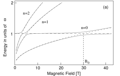
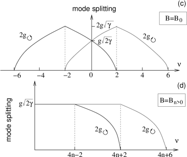
Figure 2: (a) Coupled phonon and magneto-excitons as a function of the magnetic field. Energies are in units of the bare phonon energy $\omega$. Dashed lines indicate the uncoupled valley-symmetric modes, with $g_{\mathcal{A}}=0$. (b) Mode splitting as a function of the filling factor, as may be seen in Raman spectroscopy, with the resonance condition $\Omega_{n=0}\approx\tilde{\omega}_{0}$, for $\nu=0$ in (I), $0<|\nu|<2$ (in II), and $\nu=\pm 2$ (in III). The absolute intensity of the modes is in arbitrary units, but the height and the width reflect the expected relative intensities. (c) Mode splitting for $n=0$, as a function of the filling factor $\nu$. (d) Same as in (c) for $n\geq 1$.

A generic form of the phonon-magnetoexciton anticrossing and formation of coupled modes, $\omega_{\mathcal{A}}^{\pm}(n)$ in undoped graphene (i.e., $\nu=0$) is illustrated in Fig. 2(a). Such an anticrossing and mode mixing is simlar to that described by Ando AndoMP . It can manifest itself in Raman spectroscopy: in a fine structure acquired by the G-line (earlier attributed pisana ; yan ; ferrari ; gupta ; graf to the in-plane optical phonon at the $\Gamma$-point, E_2g mode) at the magneto-phonon resonance conditions. The effect is the strongest for the resonance $\Omega_{n=0}\approx\tilde{\omega}_{0}$ between the phonon and magnetoexciton based upon $-,1\Rightarrow 0$ and $0\Rightarrow+,1$ transitions. When approaching the resonance (by sweeping a magnetic field), the phonon line becomes accompanied by a weak satellite moving towards it and increasing its intensity. Exactly at the magnetophonon resonance, where both the upper mode [$\tilde{\omega}_{\mathcal{A}}^{+}(n)$] and the lower mode [$\tilde{\omega}_{\mathcal{A}}^{-}(n)$] consist of an equal-weight superposition of the phonon and the resonant exciton, with $\cos\theta=\sin\theta=1/\sqrt{2}$, the G-band in graphene would appear as two lines. For $\Omega_{n=0}=\sqrt{2}v/\lambda_{B}\approx 36\sqrt{B\mathrm{[T]}}$ meV (see footnote2 ; AndoMP ) and $\tilde{\omega}_{0}\simeq 200$ meV, this resonance occurs in an experimentally accessible field range, $B_{0}\simeq 30$ T. For the filling factor $\nu=0$, the central LL ($n=0$) is always half-filled. Then, coupling and, therefore, splitting of the $\circlearrowright$- and $\circlearrowleft$-polarized modes coincide, $g_{\circlearrowright}=g_{\circlearrowleft}$, thus, giving rise to a pair of peaks at the energies $\tilde{\omega}^{\pm}=\tilde{\omega}_{0}\pm g_{\circlearrowright}$ sketched in part I in Fig. 2(b). For the magnetic field value $B_{0}\simeq 30$ T and $g\simeq 0.28$eV lazzeri , we estimate this splitting as $2g_{\mathcal{A}}\sim 16$meV ($\sim 130$cm^-1), which largely exceeds the G-band width observed in Refs. pisana ; yan ; ferrari ; gupta ; graf .

Doping of graphene changes the strength of the coupling constants $g_{\circlearrowright}\$and $g_{\circlearrowleft}$, as shown in Fig. 2(c). This is because a higher (lower) occupancy of the $n=0$ LL reduces (enhances) the oscillator strength of the $\circlearrowleft$ polarized transition due to the availability of filled and empty states in the involved LLs, whereas the same change in the electron density has the opposite effect on $g_{\circlearrowright}$. As a result, for an arbitrary filling factor $-2<\nu<2$, we predict that, in the vicinity of magnetophonon resonance, the phonon mode (and, therefore, G-band in Raman spectrum) should split into four lines [part II in Fig. 2(b)], with $\tilde{\omega}_{\circlearrowright}^{\pm}=\tilde{\omega}\pm g_{\circlearrowright}$ for $\circlearrowright$-polarized and $\tilde{\omega}_{\circlearrowleft}^{\pm}=\tilde{\omega}\pm g_{\circlearrowleft}$ for $\circlearrowleft$-polarized phonons. In the quantum Hall state at filling factor $\nu=2$, the transition $-,1\Rightarrow 0$ becomes successively blocked and no longer affects the frequency of a $\circlearrowleft$-polarized phonon, whereas the transition $0\Rightarrow+,1$ acquires the maximum strength, thus, increasing the coupling parameter $g_{\circlearrowright}$. This leads to the magnetophonon resonance fine structure consisting of three peaks, with an even larger splitting between side lines, as sketched in part III in Fig. 2(b). Interestingly, this may enable one to directly observe lattice modes with a definite circular polarization. A further increase of the electron filling factor reduces the side-line splitting which should completely disappear at $\nu=6$, after the transition $0\Rightarrow+,1$ becomes blocked by a complete filling of the $+,1$ LL [Fig. 2(c)]. The same arguments hold for p-doped graphene, though in this case the roles of $\circlearrowright$- and $\circlearrowleft$-polarized modes are interchanged.

Magnetophonon resonances with other possible inter-LL transitions $n\Rightarrow n+1$ occur at much lower magnetic fields, $B_{n}=B_{0}/(\sqrt{n}+\sqrt{n+1})^{2}$. For example, a resonant phonon coupling with the magnetoexciton $\psi_{\mathcal{A};as}(1)$ is expected to occur at $B_{1}\approx 5$T. Its description remains qualitatively similar, though for $n>0$ the mode splitting is less pronounced because of the $B$-field dependence of the coupling constants in Eq. (3). One finds that $g_{\circlearrowright}=g_{\circlearrowleft}$ for $|\nu|<2(2n-1)$. At $\nu=2(2n-1)$, filling of the $n$-th LL starts changing, which reduces splitting of the $\circlearrowleft$-polarized mode and gives rise to the four-peak structure. At $\nu=2(2n+1)$, where the $+,n$ LL becomes completely filled, splitting of the $\circlearrowleft$-polarized phonon vanishes, thus, resulting in the three-peak fine structure [part III in Fig. 2(b)] that would persist up to $\nu=2(2n+3)$. This is because the splitting of the $\circlearrowright$-polarized modes remains constant up to the filling factor $\nu=2(2n+1)$, above which population of the $+,(n+1)$ LL starts to suppress the value of $g_{\circlearrowright}$, until the latter vanishes at $\nu=2(2n+3)$ [see Fig. 2(d)].

In conclusion, we have predicted a filling-factor dependence of the fine structure acquired by the in-plane (E_2g) optical phonon in graphene when the latter is in resonance with one of the inter-LL transitions in this material. The effect is expected to be most pronounced when the phonon is resonantly coupled to the $0\Rightarrow+,1$ and $-,1\Rightarrow 0$ transitions, which requires a magnetic field $B_{0}\simeq 30$T. The predicted mode splitting may be used to measure directly the strength of the electron-phonon coupling, and also to distinguish between circularly (left- and right- hand) polarized lattice modes.

We thank D. Abergel, A. Ferrari, P. Lederer, and A. Pinczuk for useful discussions. This work was suported by Agence Nationale de la Recherche Grant ANR-06-NANO-019-03 and EPSRC-Lancaster Portfolio Partnership EP/C511743. We thank the MPI-PKS workshop ‘Dynamics and Relaxation in Complex Quantum and Classical Systems and Nanostructures’ and the Kavli Institute for Theoretical Physics, UCSB (NSF PHY99-07949) for hospitality.

Erratum

In the previous version (v3) of this Letter, we have underestimated the numerical value of the mode splitting of the magnetophonon resonance [see paragraph after Eq. (5)] by a factor of $2$ (the text above takes into account the corrected parameters). This is a result of two mistakes. First, there is a factor of $\sqrt{2}$, which finds its origin in an erroneous normalization of the circular polarized phonons. They should indeed be defined as $u_{\circlearrowleft}=(u_{x}+iu_{y})/\sqrt{2}$ and $u_{\circlearrowright}=(u_{x}-iu_{y})/\sqrt{2}$ [and not as $u_{\circlearrowleft}=u_{x}+iu_{y}$ and $u_{\circlearrowright}=u_{x}-iu_{y}$ as incorrectly assumed on page 1, second column], such that the associated phonon operators $b_{\mathcal{A}}$ obey the usual commutation relations $[b_{\mathcal{A}},b_{\mathcal{A}^{\prime}}^{\dagger}]=\delta_{\mathcal{A},\mathcal{A}^{\prime}}$, with $\mathcal{A}=\circlearrowleft,\circlearrowright$. This yields a factor of $\sqrt{2}$ in the definition of the effective coupling constants [Eq. (3)], which read in the corrected form

$$g_{\circlearrowleft}(n)=g\sqrt{(1+\delta_{n,0})\gamma}\sqrt{\bar{\nu}_{-,(n+1)}-\bar{\nu}_{+,n}}\ ,$$

$$g_{\circlearrowright}(n)=g\sqrt{(1+\delta_{n,0})\gamma}\sqrt{\bar{\nu}_{-,n}-\bar{\nu}_{+,(n+1)}}\ .$$

As a consequence, the zero-field dimensionless coupling constant $\lambda$ [defined in the first column page 3 of our Letter] is multiplied by a factor of 2 and becomes $\lambda=(2/\sqrt{3}\pi)(g/t)^{2}$.

Second, we also underestimated the numerical value of the electron-phonon coupling constant $g$ by a factor of $\sqrt{2}$. Indeed, $g$ defined in our work [see Eq. (1)] is related to $\langle g_{\Gamma}^{2}\rangle_{F}\simeq 0.0405$ eV² computed by Piscanec et al. piscanecbis as $g=\sqrt{2\langle g_{\Gamma}^{2}\rangle_{F}}\simeq 0.28$ eV and not as $g=\sqrt{\langle g_{\Gamma}^{2}\rangle_{F}}\simeq 0.2$ eV as incorrectly assumed in our Letter. In addition, there is a substantial uncertainty in the precise value of the constant $g$. In a tight-binding model, the latter may be related to the derivative of the hopping amplitude $t$ as a function of the carbon-carbon distance $a$ as $g=(-dt/da)\times 3/(2\sqrt{M\omega})$ andobis . Harrison’s phenomenological law $t\propto 1/a^{2}$ then implies that $g\simeq 0.26$ eV. Experiments in graphene pisanabis and yanbis in zero magnetic field give for the dimensionless coupling constant $\lambda$ the values $4.4\times 10^{-3}$ and $5.3\times 10^{-3}$ respectively. This determines $g$ in between $0.3$ eV and $0.36$ eV, where we take into account that the value of $t$ lies between $2.7$ and $3$ eV. In the end, we have to take $g$ in the range between $0.26$ and $0.36$ eV [instead of $g\simeq 0.2$ eV] and therefore the dimensionless coupling constant becomes $\lambda\simeq(2.8\textrm{ to }5.3)\times 10^{-3}$ [instead of $\lambda\simeq 10^{-3}$].

As a result of the two factors of $\sqrt{2}$, the numerical estimate for the mode splitting $2g_{\mathcal{A}}$ at $\nu=0$ and $B\simeq 30$ T [at the discussed resonance $-,1\Rightarrow 0$ and $0\Rightarrow+,1$, see second column of page 3] becomes $2g_{\mathcal{A}}\sim 15$ meV ($\sim 120$ cm^-1), for $g\simeq 0.26$ eV and $2g_{\mathcal{A}}\sim 20$ meV ($\sim 160$ cm^-1) for $g\simeq 0.36$ eV [instead of $2g_{\mathcal{A}}\sim 8$ meV]. The effect is therefore twice larger than initially predicted. The conclusions of our work remain unaltered.

We would like to thank C. Faugeras and M. Potemski for having drawn our attention on the underestimated value of the mode splitting. See also their recent preprint where they measure the magnetophonon resonance faugerasbis .

References

- (1) W. Kohn, Phys. Rev. Lett. 2, 393 (1959).
- (2) G.D. Mahan, Many-Particle Physics, Kluwer Academic, New York 2000.
- (3) K. Novoselov et al., Science 306, 666 (2004).
- (4) K. Novoselov et al., Nature 438, 197 (2005).
- (5) Y. Zhang et al., Nature 438, 201 (2005).
- (6) Y. Zhang et al., Phys. Rev. Lett. 96, 136806 (2006).
- (7) K. Novoselov et al., Nature Phys. 2, 177 (2006).
- (8) S. Pisana et al., Nat. Mater. 6, 198 (2007).
- (9) J. Yan, Y. Zhang, P. Kim, and A. Pinczuk, Phys. Rev. Lett. 98, 166802 (2007).
- (10) T. Ando, J. Phys. Soc. Jpn. 75, 124701 (2006).
- (11) A.H. Castro Neto and F. Guinea, Phys. Rev. B 75, 045404 (2007).
- (12) M. Lazzeri and F. Mauri, Phys. Rev. Lett. 97, 266407 (2006).
- (13) J.W. McClure, Phys. Rev. 104, 666 (1956).
- (14) J.P. Maneval, A. Zylberzstejn, and H.F. Budd, Phys. Rev. Lett. 23, 848 (1969); G. Bauer and H. Kahlert, Phys. Rev. B 5, 566 (1972).
- (15) R.J. Nicholas, S.J. Sessions, and J.C. Portal, Appl. Phys. Lett. 37, 178 (1980); T.A. Vaughan et al., Phys. Rev. B 53, 16481 (1996).
- (16) T. Ando, J. Phys. Soc. Jpn 76, 024712 (2007).
- (17) A.C. Ferrari et al., Phys. Rev. Lett. 97, 187401 (2006).
- (18) A. Gupta et al., Nano Lett. 6, 2667 (2006).
- (19) D. Graf et al., Nano Lett. 7, 238 (2007).
- (20) A. Iyengar et al., Phys. Rev. B 75, 125430 (2007).
- (21) M.L. Sadowski et al., Phys. Rev. Lett. 97, 266405 (2006).
- (22) D.S.L. Abergel and V. I. Fal’ko, Phys. Rev. B 75, 155430 (2007).
- (23) Numerical results yield eV; S. Piscanec et al., Phys. Rev. Lett. 93, 185503 (2004).
- (24) We use the reported value cm/s; A.K. Geim and K.S. Novoselov, Nat. Mater. 6, 183 (2007).
- (25) P.R. Wallace, Phys. Rev. 71, 622 (1947).
- (26) R. Saito, G. Dresselhaus, M.S. Dresselhaus, Physical Properties of Carbon Nanotubes, Imperial College Press, London 1998.
- (27) T. Ando, J. Phys. Soc. Jpn. 74, 777 (2005).
- (28) The electron-phonon coupling is off-diagonal because a lattice distortion affects the bond length and thus the nearest-neighbor hopping between the two different sublattices castroneto ; ando .

References

- (1) T. Ando, J. Phys. Soc. Jpn 75, 124701 (2006); ibid 76, 024712 (2007).
- (2) S. Piscanec, M. Lazzeri, F. Mauri, A. C. Ferrari, and J. Robertson, Phys. Rev. Lett. 93, 185503 (2004).
- (3) S. Pisana, M. Lazzeri, C. Casiraghi, K. S. Novoselov, A. K. Geim, A. C. Ferrari, and F. Mauri, Nature Materials 6, 198 (2007).
- (4) J. Yan, Y. Zhang, P. Kim, and A. Pinczuk, Phys. Rev. Lett. 98, 166802 (2007).
- (5) C. Faugeras, M. Amado, P. Kossacki, M. Orlita, M. Sprinkle, C. Berger, W.A. de Heer and M. Potemski, arXiv:0907.5498.