The Spitzer c2d Survey of Large, Nearby, Insterstellar Clouds. IX. The Serpens YSO Population As Observed With IRAC and MIPS

Abstract

We discuss the results from the combined IRAC and MIPS c2d Spitzer Legacy observations of the Serpens star-forming region. In particular we present a set of criteria for isolating bona fide young stellar objects, YSO’s, from the extensive background contamination by extra-galactic objects. We then discuss the properties of the resulting high confidence set of YSO’s. We find 235 such objects in the 0.85 deg² field that was covered with both IRAC and MIPS. An additional set of 51 lower confidence YSO’s outside this area is identified from the MIPS data combined with 2MASS photometry. To understand the properties of the circumstellar material that produces the observed infrared emission, we describe two sets of results, the use of color-color diagrams to compare our observed source properties with those of theoretical models for star/disk/envelope systems and our own modeling of the subset of our objects that appear to be well represented by a stellar photosphere plus circumstellar disk. These objects exhibit a very wide range of disk properties, from many that can be fit with actively accreting disks to some with both passive disks and even possibly debris disks. We find that the luminosity function of YSO’s in Serpens extends down to at least a few $\times 10^{-3}$ L_⊙ or lower for an assumed distance of 260 pc. The lower limit may be set by our inability to distinguish YSO’s from extra-galactic sources more than by the lack of YSO’s at very low luminosities. We find no evidence for variability in the shorter IRAC bands between the two epochs of our data set, $\Delta t\sim$ 6 hours. A spatial clustering analysis shows that the nominally less-evolved YSO’s are more highly clustered than the later stages and that the background extra-galactic population can be fit by the same two-point correlation function as seen in other extra-galactic studies. We also present a table of matches between several previous infrared and X-ray studies of the Serpens YSO population and our Spitzer data set. The clusters in Serpens have a very high surface density of YSOs, primarily with SEDs suggesting extreme youth. The total number of YSOs, mostly Class II, is greater in the region outside the clusters.

1 Introduction

The Serpens star-forming cloud is one of five such large clouds selected for observation as part of The Spitzer Legacy project “From Molecular Cores to Planet-forming Disks” (c2d) (Evans et al., 2003). Previous papers in this series have described the observational results in the Serpens Cloud as seen with IRAC (Harvey et. al., 2006)(Paper I) and MIPS (Harvey et al., 2007) as well as some of the other clouds (Jorgensen et al., 2006; Rebull et al., 2006). In this paper we examine how the combination of the IRAC and MIPS data together with other published results on this region can be used to find and characterize a highly reliable catalog of young stellar objects (YSO’s) in the surveyed area. With the combination of broad wavelength coverage and amazing depth of Spitzer’s sensitivity we are able to probe to both extremely low luminosity limits for YSO’s and to cover a very wide range in dust emission, both in optical depth and in range of emitting temperatures. The Spitzer wavelength region is particularly well tuned for sensitivity to dust at temperatures appropriate for solar-system size disks around young stars.

The region of the Serpens Cloud mapped in our survey is an area rich in star formation. Eiroa, Djupvik & Casali (2007) have extensively reviewed studies at a variety of wavelengths of this area. There is evidence from previous observations of strong clustering (Testi et al., 2000; Testi & Sargent, 1998), dense sub-mm cores (Casali, Eiroa & Duncan, 1993; Enoch et al., 2007), and high-velocity outflows (Ziener & Eisloffel, 1999; Davis et al., 1999). Pre-Spitzer infrared surveys of the cloud have been made by IRAS (Zhang et al., 1988; Zhang, Laureijs, & Clark, 1988) and ISO (Kaas et al., 2004; Djupvik et al., 2006) as well as the pioneering ground-based surveys that first identified it as an important region of star formation (Strom, Vrba & Strom, 1976). Using MIPS and all four bands of IRAC the c2d program has mapped a 0.85 deg² portion of this cloud that includes a very well-studied cluster of infrared and sub-millimeter sources (Eiroa & Casali, 1992; Hogerheijde, van Dishoeck, & Salverda, 1999; Hurt & Barsony, 1996; Harvey, Wilking, & Joy, 1984; Testi & Sargent, 1998). At its distance of $260\pm 10$ pc (Straizys, Cernis, & Bartasiute, 1996) this corresponds to an area of about 2.5 $\times$ 9 pc. In paper I we identified at least two main centers of star formation as seen by Spitzer in this cloud, that we referred to as Cluster A and B. Cluster A is the very well-studied grouping also commonly referred to as the Serpens Core. Cluster B was the subject of a recent multi-wavelength study by Djupvik et al. (2006), who referred to it as the Serpens G3-G6 cluster.

The 235 YSO’s with high signal-to-noise that we have catalogued constitute a sufficiently large number that we can examine statistically the numbers of objects in various evolutionary states and the range of disk properties for different classes of YSO’s. We characterize the circumstellar material with color-color diagrams that allow comparison with other recent studies of star-forming regions, and we model the energy distributions of the large number of YSO’s that appear to be star$+$circumstellar disk systems. We are able to construct the YSO luminosity function for Serpens since we have complete spectral coverage for all the sources over the range of wavelengths where their luminosity is emitted, and we are able to characterize the selection effects inherent in the luminosity function from comparison with the publicly available and signicantly deeper SWIRE survey (Surace et al., 2004). We find that the population of YSO’s extends down to luminosities below $10^{-2}$ L_⊙, and we discuss the significance of this population. Our complete coverage in wavelength and luminosity space also permits us to discuss the spatial distribution of YSO’s to an unprecedented completeness level. We note also that, unlike the situation discussed by Jorgensen et al. (2006) for Perseus, in Serpens there do not appear to be any very deeply embedded YSO’s that are not found by our YSO selection criteria.

In §2 we briefly review the observational details of this program and then in §3 we describe in detail the process by which we identify YSO’s and eliminate background contaminants. In §4 we describe a search for variability in our dataset. We compare our general results on YSO’s with those of earlier studies of the Serpens star-forming region in §5. We discuss in §6 the YSO luminosity function in Serpens and, in particular, the low end of this function. We next analyze the spatial distribution of star formation in the surveyed area and compare it to the distribution of dust extinction as derived from our observations in §7. In §8 we construct several color-color diagrams that characterize the global properties of the circumstellar material and show modeling results for a large fraction of our YSO’s that appear to be star$+$disk systems. Finally, §9 discusses several specific groups of objects including the coldests YSO’s and a previously identified “disappearing” YSO. We also mention several obvious high-velocity outflows from YSO’s that will certainly be the subject of further study.

2 Observations

The parameters of our observations have already been described in detail in Paper I for IRAC and in a companion study (Harvey et al., 2007) for MIPS. We summarize here some of the issues most relevant to this study.

We remind the reader that the angular resolution of the Spitzer imaging instruments varies widely with wavelength, since Spitzer is diffraction limited longward of $\lambda\sim 10$µm. In the shorter IRAC bands the spatial resolution is of order 2″, while from 24–160µm, it goes from roughly 5″ to 50″. The area chosen for mapping was defined by the $A_{V}>6$ contour in the extinction map of Cambrésy (1999) and by practical time constraints (Evans et al., 2003). With the exception of a small area of 0.04 deg² on the northeast edge of the IRAC map, all of the area mapped with IRAC was also covered with MIPS at both 24 and 70µm, and most of it at 160µm. As described by Harvey et al. (2007), some substantial additional area was observed with MIPS without matching IRAC observations. In this current paper we restrict our attention to only the area that was observed from 3.6 to 70µm, 0.85 deg². This entire region was observed from 3.6 to 24µm at two epochs, with a time separation of several hours to several days, but at only one epoch at 70µm. We also specifically do not include the 160µm observations in our discussion because they did not cover the entire area and because most of the YSO’s in Serpens are too closely clustered to be distinguishable in the large beam of the 160µm data. Harvey et al. (2007) discuss briefly the extended 160µm emission in this region and the four point-like sources found at 160µm. Figure 1 shows the entire area mapped with all four IRAC bands and MIPS at 24 and 70µm and also indicates the locations of several areas mentioned in the text.

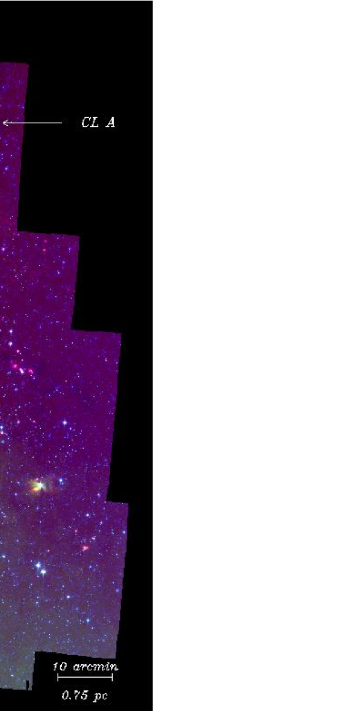
Figure 1: Three color image of the area mapped in Serpens. The color mapping is: blue/4.5µm, green/8.0µm, and red/24µm. The locations of Cluster A (Core Cluster), Cluster B (Serpens G3-G6 Cluster), and VV Ser are indicated.

In addition to this area of the Serpens cloud defined by relatively high A_V, we also observed small off-cloud regions around the molecular cloud with relatively low A_V in order to determine the background star and galaxy counts. The area of combined IRAC/MIPS coverage of these off-cloud regions, however, was relatively small and so these observations are not discussed further in this paper. As detailed below, we have used the much larger and deeper SWIRE (Surace et al., 2004) survey to understand the characteristics of the most serious background contaminants in our maps, the extra-galactic objects.

3 YSO Selection

Paper I described a process for classifying infrared objects into several categories: those whose energy distributions could be well-fitted as reddened stellar photospheres, those that had a high likelihood of being background galaxies, and those that were viable YSO candidates. We have refined this process by combining MIPS and IRAC data together as well as by producing an improved comparison catalog from the SWIRE (Surace et al., 2004) survey, trimmed as accurately as possible to the c2d sensitivity limits. As shown by the number counts versus Wainscoat models of the Galactic background toward Serpens in paper I, nearly all the sources observed in our survey are likely to be background stars. Because of the high sensitivity of IRAC channels 1 and 2 relative to both 2MASS and to IRAC channels 3 and 4, most of the more than 200,000 sources extracted from our Serpens dataset do not have enough spectral coverage for any reliable classification algorithm. In particular, “only” 34,000 sources had enough spectral information from a combination of 2MASS and IRAC data to permit a test for consistency with a stellar photosphere-plus-extinction model, and nearly 32,000 of these objects were classified as reddened stellar photospheres. These normal stellar objects are not considered further in our discussion and are not plotted on the various color and magnitude diagrams. The details of this classification process and the criteria for fitting are described in detail by Evans et al. (2007).

In order to pursue the classification process for YSO’s beyond that described in Paper I, we added one more step to the data processing described there. This final step was “band-filling” the catalog to obtain upper limits or low S/N detections of objects that were not found in the original source extraction processing. This step is described in detail in the delivery documentation for the final c2d data delivery (Evans et al., 2007). In short, though, it involved fixing the position of the source during an extraction at the position of an existing catalog source and fitting the image data at that fixed position for two parameters, a background level and source flux, assuming it was a point source. For this processing step, the fluxes of all the originally extracted sources were subtracted from the image first. In the case of the data discussed in this paper, the most important contribution of this band-filling step is to give us flux estimates for the YSO candidates and extra-galactic candidates at 24µm. Because our knowledge of the true PSF is imperfect and because the 24µm PSF is so much larger than the IRAC ones, it was also necessary to examine these results carefully to be sure a band-filled 24µm flux was not simply the poorly subtracted wings of a nearby bright source that, in fact, completely masked the source being band-filled. For the purposes of this paper, all upper limits are given as 5$\sigma$ values.

Three of the sources eventually selected as YSO’s by the process described below had 24µm fluxes that were obviously saturated. These are the objects in Table A numbered 127, 137, and 182. For these three objects we derived the 24µm flux from a fit to the wings of the source profiles, rather than a fit to the whole profile as is done by the standard c2d source extraction.

3.1 Constructing a Control Catalog from Deep Extragalactic SWIRE Observations

We use the IRAC and MIPS images of the ELAIS N1 field obtained by the SWIRE team as a control field for understanding the extragalactic population with colors that mimic those of YSOs present in our Serpens field. This SWIRE field, expected to contain no extinction from a molecular cloud and no YSOs, has coverage by both IRAC and MIPS of 5.31 deg² and has a limiting flux roughly a factor of four below that of our observations of Serpens. The analysis described below is designed to produce a resampled version of the SWIRE field as it would have been observed with the typical c2d sensitivity and as if it were located behind a molecular cloud with the range of extinctions observed in Serpens. The process of simulating these effects is discussed in detail in the final c2d data delivery documentation (Evans et al., 2007), but the steps are summarized here.

To avoid effects that may result from differences in data processing, the BCD images for this SWIRE field were processed by our pipeline in exactly the same way as our own observations. Once a bandmerged catalog of SWIRE sources was constructed, we first simulated the reddening of sources that would occur if Serpens had been in the foreground of this field. This reddening was accomplished by randomly applying extinction to each SWIRE source according to the extinction profile of Serpens, shown in Figure 2. For example, $\sim$23% of SWIRE sources were randomly selected and visual extinctions in the range 6.5 $\leq\ A_{V}<$ 7.5 were applied, $\sim$19% of sources were extincted by extinctions in the range 7.5 $\leq\ A_{V}<$ 8.5, and so forth. The extinctions were applied to each of the infrared bands according to the extinction law appropriate for molecular clouds and cores (Huard et al., in prep.).

Second, we degraded the sensitivity of the reddened SWIRE photometry to match that of our Serpens observations. This was accomplished by matching the detection rates as a function of magnitude in each of the bands. The 90% completeness limits of the Serpens observations are approximately 16.6, 15.6, 15.0, 16.6, 16.2, 15.2, 13.4, and 9.6 mag at J, H, K, [3.6], [4.5], [5.8], [8.0], and [24], respectively. Thus, for each band, all reddened SWIRE sources brighter than the completeness limit in Serpens would be detectable by c2d-like observations and are identified as such in the resampled SWIRE catalog. Most, but not all, sources fainter than the completeness limit will not be detected by c2d-like observations. We randomly select which sources to identify as detections, in a given band, in such as way as to reproduce the empirically determined shape of the completeness function. This resampling process is performed for each band, resulting in those sources fainter than the completeness limits in some bands being detected or not detected with the same probabilities as those for similar sources in Serpens. The photometric uncertainties of all sources in the resampled catalog of reddened SWIRE sources are re-assigned uncertainties similar to those of Serpens sources with similar magnitudes.

Finally, each source in the resampled SWIRE catalog is re-classified, based on its degraded photometry, e.g. “star”, “YSOc”, “GALc”, …. The magnitudes, colors, and classifications of sources in this resampled SWIRE catalog are then directly comparable to those in our Serpens catalog and may be used to estimate the population of extragalactic sources satisfying various color and magnitude criteria. At this level of the classification, the terms YSOc and GALc imply candidate classification status.

Figure 2: The distribution of visual extinctions found toward the roughly 50,000 sources classified as stars in our Serpens observations.

3.2 Classification Based on Color and Magnitude

In Paper I we described a simple set of criteria that basically categorized all objects that were faint and red in several combinations of IRAC and MIPS colors as likely to be galaxies (after removal of normal reddened stars). In our new classification we have extended this concept to include the color and magnitude spaces in Figure 3 together with several additional criteria to compute a proxy for the probability that a source is a YSO or a background galaxy. Figure 3 shows a collection of three color-magnitude diagrams and one color-color diagram used to classify the sources found in our 3.6 to 70$\mu$m survey of the Serpens Cloud that had S/N $\geq$ 3 in all the Spitzer bands between 3 and 24$\mu$m and that were not classified as reddened stellar photospheres. In addition to the Serpens sources shown in the left panels, the comparable set of sources from the full-sensitivity SWIRE catalog are shown in the center panels, and the sources remaining in the extincted/sensitivity-resampled version of the SWIRE catalog described above are shown in the right panels. The exact details of our classification scheme are described in Appendix A. Basically we form the product of individual probabilities from each of the three color-magnitude diagrams in Figure 3 and then use additional factors to modify that total “probability” based on source properties such as: its K - [4.5] color, whether it was found to be extended in either of the shorter IRAC bands, and whether its flux density is above or below some empirically determined limits in several critical bands. Table 1 summarizes the criteria used for this class separation. The cutoffs in each of the color-magnitude diagrams and the final probability threshold to separate YSO’s from extragalactic objects were chosen: (1) to provide a nearly complete elimination of all SWIRE objects from the YSO class, and (2) to maximize the number of YSO’s selected in Serpens consistent with visual inspection of the images to eliminate obvious extragalactic objects (such as a previously uncatalogued obvious spiral galaxy at RA = 18h 29m 57.4s , Dec = +00^∘ 31’ 41” J2000 ).

The cutoffs in color-magnitude space were constructed as smooth, exponentially decaying probabilities around the dashed lines in each of the three diagrams. Sources far below the lines were assigned a high probability of being extra-galactic contamination with a smoothly decreasing probability to low levels well above the lines. In the case of the [24] versus [8.0]-[24] relation, the probability dropped off radially away from the center of the elliptical segment shown in the figure. After inclusion of these three color-magnitude criteria, we added the additional criteria listed in Table 1. These included: (1) a factor dependent on the K - [4.5] color, $Prob/(K-[4.5])$, to reflect the higher probability of a source being an extra-galactic (GALc) contaminant if it is bluer in that color, (2) a higher GALc probability for sources that are extended at either 3.6 or 4.8$\mu$m where our survey had the best sensitivity and highest spatial resolution, (3) a decrease in GALc probability for sources with a 70$\mu$m flux density above 400 mJy, empirically determined from examination of the SWIRE data, and (4) identification as “extragalactic” for any source fainter than [24] = 10.0. Again, we emphasize that these criteria are based only on the empirical approach of trying to characterize the SWIRE population in color-magnitude space as precisely as possible, not on any kind of modeling of the energy distributions.

Figure 4 graphically shows the division between YSO’s and likely extragalactic contaminants. The number counts versus our “probability” are shown for both the Serpens cloud and for the resampled SWIRE catalog (normalized to the Serpens area). This illustrates how cleanly the objects in the SWIRE catalog are identified by this probability criterion. In the Serpens sample there are clearly two well-separated groups of objects plus a tail of intermediate probability objects that we have mostly classified as YSO’s since no such tail is apparent in the SWIRE sample.

Our choice of the exact cut between “YSO” and “XGal” in Figure 4 is somewhat arbitrary because of the low level tail of objects in Serpens in the area of log(probability) $\sim$ -1.5. Since the area of sky included in our SWIRE sample is more than six times as large as the mapped area of Serpens, we chose our final “probability” cut, $log(P)\leq-1.47$, to allow two objects from the full (not resampled) SWIRE catalog into the “YSO” classification bin. Thus, aside from the vagaries of small-number statistics, we expect of order 0 – 1 extragalactic interlopers in our list of Serpens YSO’s. The right panels in Figure 3, which use the resampled version of the SWIRE catalog, show that the effects of sensitivity and, especially, the extinction in Serpens make our cutoff limits particularly conservative in terms of likelihood of misclassification. We examined all the YSO candidates chosen with these criteria both in terms of the quality of the photometry and their appearance in the images. A significant number, $\sim$ 50 candidates were discarded because of the poor quality of the bandfilling process at 24$\mu$m due to contamination by a nearby brighter source or because of their appearance in the images. It is possible that a small number of these discarded candidates are, in fact, true YSO’s in the Serpens Cloud. We also manually classified one source as “YSO” (# 75 in Table A) that may be the exciting source for an HH-like outflow in Cluster B (see also discussion of this region by Harvey et al. (2007)), but which was not so classified because of its extended structure in the IRAC bands. Table A lists the 235 YSO’s that resulted from this selection process.

Another test of the success of our separation of background contaminants is to simply plot the locations of the YSO’s and likely galaxies on the sky. Figure 5 shows such a plot in addition to a plot of visual extinction discussed later. There is clearly a very uniform distribution of background contaminants and a quite clustered distribution of YSO’s (see further discussion in §7).

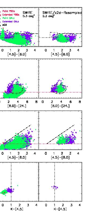
Figure 3: Color-magnitude and color-color diagrams for the Serpens Cloud (left), full SWIRE (center), and trimmed SWIRE regions. The black dashed lines show the “fuzzy” color-magnitude cuts that define the YSO candidate criterion in the various color-magnitude spaces. The red dashed lines show hard limits, fainter than which objects are excluded from the YSO category.

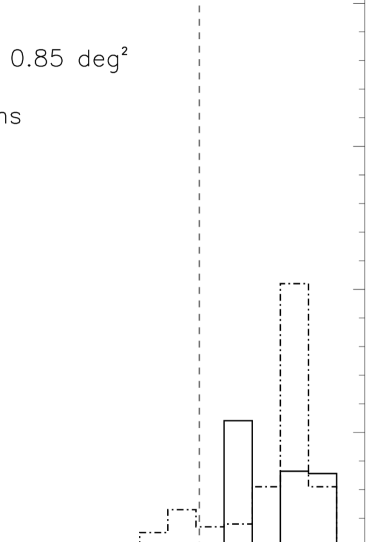
Figure 4: Plot of the number of sources versus probability (of being a background contaminant) for the Serpens cloud and for the trimmed SWIRE catalog described in the text. The vertical dashed line shows the separation chosen for YSO’s versus extra-galactic candidates. For both samples, only sources with detections in all four IRAC bands are plotted to keep the number counts of contaminants on scale!

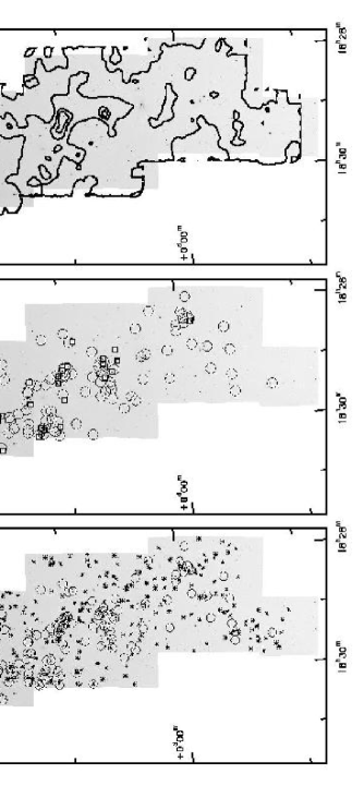
Figure 5: Left panel: image of the entire mapped area of Serpens at 8.0$\mu$m with the positions of YSO’s plotted with circles and likely extra-galactic background contaminants with asterisks; center panel: same image with YSO’s of luminosity $L<2\times 10^{-2}$L_⊙ plotted with boxes, and higher luminosity YSO’s plotted with circles; right panel: contours of visual extinction A_v at levels of 5, 10, 20, 30 magnitudes as derived from fitting the energy distributions of sources that were well-fit as reddened stellar photospheres in our data set.

There is one additional kind of contaminant that is likely to appear in our data at a relatively low level, AGB stars. The ISO observations by, for example, van Loon et al. (1999) and Trams et al. (1999) show that the range of brightnesses of AGB stars in the LMC covers a span equivalent roughly to $8<[8.0]<12$, with colors generally equivalent to $[4.5]-[8.0]<1$. Very compact proto-planetary nebulae are generally redder, but even brighter at 8$\mu$m (see e.g. Hora et al. 1996). For typical galactic AGB stars, between 5 and 15 kpc from the sun, this would imply $3<[8.0]<9$. The off-cloud fields (when normalized to the same area as the Serpens data) provide the best handle on the degree of contamination from AGB stars; in Paper I we saw one object classified as a YSO candidate in the off-cloud panel of Figure 9 with [8.0] $<$ 9. Therefore, based on the ratio of areas mapped in Serpens versus the off-cloud observations, we expect the number of AGB stars contaminating the YSO candidate list in the Serpens cloud to be of order a half dozen. As a further check, we have examined the entire set of off-cloud fields for such objects. In this combined area of 0.58 deg², there are only 3 such YSO candidates. Finally, Merín et al. (2007) have classified four AGB stars by their Spitzer-IRS spectra in the Serpens cloud; these are identified in the diagrams of Figure 3 by black open diamonds and obviously are not included in our final list of high-probability YSO’s. Statistically then, it is possible that a couple of our brightest YSO’s are in fact AGB stars. In fact, Merín et al. (2007) have obtained modest S/N optical spectra of a number of our YSO’s. They find five objects whose estimated extinction seems inconsistent with their location in the Serpens cloud and which suggests they might be background objects at much larger distances with modest circumstellar shells like AGB stars. We have indicated these five objects in Table A with a footnote “b”.

It is also interesting to ask the reverse question, to what extent have our criteria successfully selected objects that were known YSO’s from previous observations. Alcalá et al. (2007) have used the same criteria to search for YSO’s in the c2d data for Chamaeleon II. They conclude that all but one of the known YSO’s in that region are identified. In §5 we discuss the comparison of our results with several previous studies of Serpens that searched for YSO’s. Our survey found counterparts to all the previously known objects in our observed area that had $S/N>5$ in those studies, but we did not classify many of them as YSO’s because of the lack of significant excess in the IRAC or MIPS bands. Most of these were indeed suggested only as candidate YSO’s by the authors, so we do not consider this fact to be a problem for our selection criteria. We again emphasize the fact that our selection criteria for youth are based solely on the presence of an infrared excess at some Spitzer wavelength.

The total number of objects classified as YSO’s in the IRAC/MIPS overlap area of the Serpens cloud is 235. From the statistics of our classification of the SWIRE data we expect of order 1 $\pm$ 1 of these are likely to be galaxies. On the other hand, as we discuss in §6, some of the faint red objects in Figure 3 (below the dashed line) may also be young sub-stellar objects. For example, we note the case of the young brown dwarf BD-Ser 1 found by Lodieu et al. (2002) that was not selected by our criteria because of its relative faintness. Of these 235, 198 were detected in at least the H and K_s bands of the 2MASS survey at better than 7$\sigma$. The number of YSO’s in each of the four classes of the system suggested by Lada (1987) and extended by Greene et al. (1994) is: 39 Class I, 25 Class “Flat”, 132 Class II, and 39 Class III, using the flux densities available between 1 and 24$\mu$m. Because we require some infrared excess to be identified as a YSO, the Class III candidates were necessarily selected by some measurable excess typically at the longer wavelengths, 8 or 24$\mu$m. An obvious corollary is that objects identified as young on the basis of other indicators, e.g. X-ray emission, lithium abundance, but without excesses in the range of 1 – 24$\mu$m are not selected with our criteria.

3.3 YSO’s Selected By MIPS

Harvey et al. (2007) found 250 YSO candidates in the entire area mapped by MIPS at 24$\mu$m in Serpens, an area of 1.8 deg²; 51 of these are outside the IRAC/MIPS overlap area and are listed in Table A. We can make a comparison of those statistics with the YSO counts here in two ways. First in the area covered by both IRAC and MIPS24 there are 197 objects that satisfy the criteria of Harvey et al. (2007), i.e., K${}_{s}<14$, K${}_{s}-[24]>2$, $[24]<10$ and 24$\mu$m S/N $\geq 5$. Of these, 184 satisfy our more restrictive criteria in this study based on the combination of 2MASS, IRAC, and MIPS data, or 93%. We would classify the other 13 as likely background galaxies. Secondly, of the 235 YSO’s found in this study, 200 have sufficient data to be classifiable by the “mips only” criteria above, but only 167 or 84% actually meet the mips-only YSO criteria. In other words, 33 objects have been classified as high quality YSO’s in this paper in the MIPS/IRAC overlap region that did not meet the criteria based only on MIPS and 2MASS data. If these ratios can be extrapolated to the larger area covered only by MIPS, then we would expect Harvey et al. (2007) to have missed 16% (8 or 9) of the YSO’s but to have included 7% (3 or 4) that would not meet our combined IRAC/MIPS criteria. With these corrections we might have expected to find $235+56=291$ YSO’s in the entire 1.8 deg² area covered by MIPS if we had matching IRAC observations. Finally, in light of our earlier discussion of AGB contaminants, it is possible that 6 – 9 of these YSO’s would actually be found to be background AGB stars.

4 Search for Variability

The fact that our data were taken in two epochs separated by 6 hours or more gives us the opportunity to search for variability over that time scale. Rebull et al. (2006) and Harvey et al. (2007) have performed similar tests for variability of the 24$\mu$m emission from sources in the c2d observations of Perseus and Serpens and found no reliable evidence for variability at that wavelength. There is, however, substantial evidence for short term variability in the near-infrared for YSO’s. We, therefore, performed a similar investigation in the two shortest IRAC bands, 3.6 and 4.5$\mu$m. No clear evidence was found at the level of $\pm$ 25% for any sources in the field over the 6-hour time scale of our multi-epoch observations.

5 Comparison with Previous Studies of Serpens

We have cross-correlated our source catalog with those from previous studies of Serpens that searched for YSO’s. We chose three studies that covered much of Cluster A at both near-IR, ISO, and X-ray wavelengths (Eiroa & Casali, 1992; Kaas et al., 2004; Preibisch, 2003), and one recent ISO study of Cluster B (Djupvik et al., 2006). Table A lists the sources from each of these previous studies and the best-matching Spitzer source from our complete catalog. In brief, we find good matches for essentially all the previous IR-selected YSO’s that had S/N $>$ 4 in the earlier studies and which were included in our mapped area. In detail, however, a number of YSO candidates from the earlier studies were not classified as YSO’s in our study. The reasons for this are different for the various catalogs. From the X-ray catalog of Preibisch (Preibisch, 2003) in Cluster A, we only identified 17 of the 45 X-ray sources as YSO’s on the basis of their infrared excesses. The X-ray sources that were not identified as YSO’s included both many objects that were well-fitted as reddened stellar photospheres (21 sources) and objects with some likely infrared excess but too little to fit our criteria aimed at eliminating extra-galactic interlopers. The situation with the infrared catalogs is somewhat different. Examining our non-matches from the ground-based study of Eiroa & Casali (1992), we find that a large fraction of their YSO’s are classified as such by our criteria, but not all. From the ISO surveys (Kaas et al., 2004; Djupvik et al., 2006) we typically identify $\sim$50–60% as YSO’s. The ones that we do not classify as such are typically those with low S/N in the ISO observations or where the amount of infrared excess was not large enough to satisfy our test of whether the object could not be fitted as an extincted stellar photosphere as described by Evans et al. (2007).

6 Luminosities

6.1 The YSO Luminosity Function in Serpens

One of the most important physical parameters for any star is its mass. For pre-main-sequence stars this is problematic, because the determination of mass depends on the placement of the star on an HR diagram and the use of model evolutionary tracks for which there is significant uncertainty at the level of at least a factor of 1.5 – 2 in the literature (Hillenbrand & White, 2004; Stassun et al., 2004). For young stars in a cluster, a poor, but still useful proxy for mass is the stellar luminosity since it is possible that most of the stars have formed more or less simultaneously. With all these caveats in mind, we display in Figure 6 the histogram of total luminosities for the 235 YSO’s found in Serpens in our survey with the assumed distance of 260 pc. We remind the reader that these objects were selected specifically on the basis of infrared excess emission, so this list is limited to YSO’s that show substantial IR excess at least somewhere in the range of 3.5 - 70$\mu$m. For example, as we discussed in §5, a comparison of our list of YSO’s with the list of X-ray sources in Cluster A (Preibisch, 2003) showed that more than half the X-ray sources were not classified as YSO’s by our infrared excess criteria. In some sense then, it is likely that the IR-selected and x-ray-selected samples are complementary in selecting less-evolved and more-evolved samples of YSO’s respectively. The luminosity function of our IR-excess-defined YSO sample peaks at roughly $2\times 10^{-2}$ L_⊙ and drops off steeply below $10^{-2}$ L_⊙. This is interestingly equal to the luminosity of objects at the hydrogen-burning limit of 0.075 M_⊙ in the models of Baraffe et al. (2002), for objects with ages of $\sim$2 Myr, a common estimate for the age of the Serpens star forming event (Kaas et al., 2004; Djupvik et al., 2006). Of course an important question to ask is to what extent this luminosity distribution in Figure 6 is influenced by selection effects.

We can estimate the selection effects in our sample from the statistics in the SWIRE samples discussed above. The completeness limits of the full catalog are nearly 2 magnitudes fainter than the trimmed version, so we assume for simplicity that the full catalog is 100% complete down to the faintest magnitudes of interest for this test in the c2d Serpens data set. Figure 7 shows the number counts as a function of “luminosity” (all sources assumed to be at 260 pc) for three versions of our c2d-processed SWIRE catalog: 1) the full-depth catalog, 2) the catalog cut-off with c2d sensitivity limits but without added extinction, and 3) the catalog corrected for both c2d sensitivity levels and extinction in the Serpens cloud. The ratio of the second to the first version serves as a good proxy for a completeness function since it includes the effects of c2d sensitivity only. The lower panel of Figure 7 then shows this ratio as our estimate of the completeness function at the range of luminosities of Serpens YSO’s observed in Figure 6. In Figure 6, then, we also indicate how the YSO luminosity function might be adjusted to account for this estimate of our survey completeness (with an assumed completeness of 100% at the bright end). Although substantial adjustments must be made to the number counts at fainter luminosities, the general conclusion remains intact that the luminosity function peaks around $few\times 10^{-2}$ L_⊙  and drops to both lower and higher luminosities. Interestingly, if our completeness estimates are valid, there may still be a substantial population of IR excess sources down to luminosities of 10^-3 L_⊙ as was already suggested in Paper I. For example, as noted earlier in §3.2, the young brown dwarf found by Lodieu et al. (2002) was not selected as a YSO with our criteria because it was faint enough that its colors placed it into the color and magnitude ranges where extra-galactic objects begin to be prominent.

Figure 6: Luminosity function for Serpens YSO’s (solid) and estimate of correction for completeness effects (dashed).

Figure 7: Upper panel – number counts for the full SWIRE catalog as processed through the c2d pipeline for objects detected in all four IRAC bands versus those for the “trimmed” version of the catalog with completeness limits for each individual band comparable to those for c2d. Lower panel – the ratio of the two number counts, i.e. completeness factor.

6.2 The Lowest Luminosity Sources

There are 37 YSO’s with total luminosities (1 – 70$\mu$m) less than $2\times 10^{-2}$ L_⊙, without any correction for selection effects in either our observations or our selection criteria. Figure 5 presented in §3.2 shows the spatial distribution of the low (L $<2\times 10^{-2}$ L_⊙) and “high” (L $>2\times 10^{-2}$ L_⊙) luminosity YSO’s in Serpens. There does not appear to be any significant difference between these two distributions. Likewise Figure 8 shows the distribution of spectral slopes, $\alpha$, for the low luminosity sample relative to two higher luminosity samples, and Table 5 lists the average and standard deviation for the spectral slopes for three luminosity samples. Again, there is no obvious difference in the distributions within the statistical uncertainties of the samples. (See also discussion in §8.1). These two facts suggest that the mechanisms and timing of formation of these two luminosity groups may not be very different. Finally, Figure 9 shows the distribution of extinction for stars nearby each YSO. For this analysis we selected all objects within 80” of each YSO that were classified as “star” by the process described earlier. We averaged the fitted extinction values for these stars; the number of stars contributing to the average ranged from 5 to 48. This figure shows that the lower luminosity YSO’s have at least as much typical extinction as the higher luminosity ones, a fact that would be unlikely if they were mis-classified background extragalactic objects.

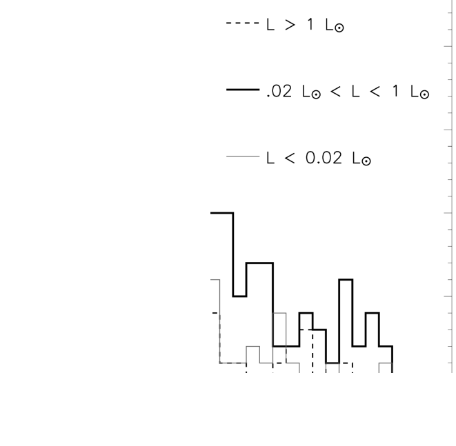
Figure 8: Histogram of distribution of spectral slopes, “alpha”, for three luminosity “classes” of YSO’s.

Figure 9: Histogram of distribution of average extinction for stars within 80” of each YSO for “high” and “low” luminosity YSO’s (above or below $2\times 10^{-2}$L_⊙).

7 Spatial Distribution of Star Formation

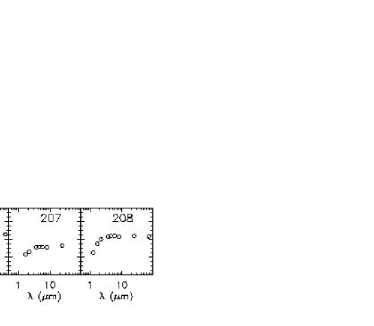
Figure 13: Spectral Energy Distributions of the Class I sources in the sample (continued). Symbols as in Figure 12.

We have already noted in §1 that the Serpens star-forming region has been identified as one displaying strong evidence of clustering of the youngest objects. We also showed in Figure 5 that the spatial distribution of our high quality YSO candidates was highly clustered. A number of authors have attempted to quantify the degree of clustering as a function of spatial scale using the two-point correlation function (Johnstone et al., 2000; Enoch et al., 2006; Simon, 1995; Gomez & Lada, 1998; Bate, Clarke & McCaughrean, 1998). Typical results have found a steep slope, $\gamma\propto d^{-2}$ on small spatial scales implying a rapid decrease in clustering on scales out to $\sim$ 10000 AU, and a substantially shallower slope, $\gamma\propto d^{-0.5}$ beyond that (Simon, 1995; Gomez & Lada, 1998). Figure 10 shows the two-point correlation function, W, for the YSO’s in our Serpens catalog and the sample of objects classified as extra-galactic background sources. The Serpens samples are divided into two groups, those with spectral slopes, $\alpha$, that place them in the Class I or “Flat” categories of Greene et al. (1994), and those whose slopes imply Class II or III. Although our range of good sampling only extends down to $\sim$ 1000 AU, equivalent to 4”, our data suggest that the slope for separations under $10^{4}$ AU is of order 0.5, and drops steeply for the more embedded and likely youngest Class I and Flat-SED objects beyond $10^{4}$ AU. The nominally more evolved objects in Class II and III, exhibit a lower level of clustering and more uniform slope in the two-point correlation function. These results are consistent with the appearance of the source distributions as shown, for example, in Figure 13 of Paper I. As shown in Figure 10, the slope and magnitude of the correlation for our sample of background extra-galactic objects is consistent with that found by, for example, Maddox et al. (1990) for a bright sample of galaxies.

The total surface density of young stellar objects in a cluster is an indicator of the richness of star formation in the cluster. Allen et al. (2006) have computed surface densities for YSO’s identified by infrared excess in a sample of 10 young clusters. They find typical peak surface densities of 500 – 1000 pc^-2 and average values of order 100 – 200 pc^-2. The peak surface density in Cluster A of our YSO’s identified by IR excess is comparable to these, of order $10^{3}$ pc^-2, and a factor of about two less in Cluster B. The average values are about a factor of 4 less than the peak in both clusters. In particular, if we define the cluster edges by the $A_{v}=20$ contour for comparison with other c2d clusters, we obtain the values in Table 6 for the number of stars per solid angle and per square parsec. We have compared the values for clusters A and B with those for the rest of the cloud and for the total cloud surveyed. The surface densities of YSOs are 10 to 20 times higher in the clusters as in the rest of the cloud. As shown by Allen et al. (2006), Cluster A in Serpens is particularly striking in terms of the contrast between the peak surface density and how quickly, within 1 pc, the density drops to very low values, $\sim few\times pc^{-2}$. In terms of volume density, though, even Cluster A has a substantially lower volume density of star formation than such rich clusters as the Trapezium (5000 pc^-3) or Mon R2 (9000 pc^-3) (Elmegreen et al. 2000).

Figure 5 also shows the spatial distribution of visual extinction in the cloud as derived from our data. These extinction values were derived from the combination of 2MASS and Spitzer data for sources that were well fit as reddened stellar photospheres as described in detail by Evans et al. (2007). As already noted in our previous studies of the IRAC data alone (Harvey et. al., 2006) and the MIPS data alone (Harvey et al., 2007), there is clearly a striking correspondence between the areas of high extinction and the densest clusters of YSO’s, particularly those containing Class I and Class Flat sources.

Figure 10: Left panel: the two-point correlation function, W, for Serpens. The dotted histogram is for sources identified as Class I and “Flat” SED objects, i.e. $\alpha\geq-0.3$. The solid histogram is for the Class II/III objects, i.e. $\alpha<-0.3$. The dashed lines show several possible power law slopes for the portions of the YSO curves. Right panel: the dashed histogram is for the objects classified as likely background galaxies with S/N $>7$ in all four IRAC bands. The dash-dot line shows the slope and amplitude found by Maddox et al. (1990) for the bright end of the extra-galactic population, which is a quite good fit to our estimate of the background contamination in our sample.

8 Disk Properties

The properties of the circumstellar dust surrounding young stars can be estimated from the overall energy distributions of the objects in a variety of ways. These properties include: the overall amount of dust, the density distribution as a function of radial distance from the central star, the morphology of the circumstellar disks which probably represent the configuration of many of these circumstellar distributions, and to some extent, the degree of evolution of the dust from typical interstellar dust to larger and more chemically evolved grains likely to represent some stage in the formation of planetary systems. We discuss several approaches to classifying the dust emission in this section, beginning with the use of infrared colors.

8.1 Color-color diagrams

Numerous authors have shown how combinations of colors in the infrared can provide significant diagnostic information on the configuration and total amount of circumstellar material around young stars. Whitney et al. (2003) modelled a wide range of disk and envelope configurations and computed their appearance in a number of infrared color-color and color-magnitude diagrams particularly relevant to Spitzer’s wavelength range. Similarly Allen et al. (2004) have published IRAC color-color diagrams for another set of models of objects with circumstellar disks and/or envelopes. Recently, Robitaille et al. (2007) have computed a very large grid of models to extend the predictions from those of Whitney et al. (2003) to a much larger parameter space. Observationally, Lada et al. (2006) have used IRAC and MIPS colors from Spitzer observations to classify the optical thickness of disks around pre-main-sequence stars in IC 348, using the terms “anemic disks” and “thick disks” to point to objects roughly in the Class III and Class II portions of the ubiquitous “Class System” (Lada, 1987; Greene et al., 1994).

Figure 11 shows three color-color diagrams and one color-magnitude diagram for the 235 Serpens YSO’s compared to the density of models from Robitaille et al. (2007) for a model cluster at the distance of Serpens with brightnesses limited to those appropriate for our sensitivity levels. For two of the diagrams the figure also indicates the approximate areas where most of the models fall for the three physical stages, I, II, and III, described by Robitaille et al. (2007) that roughly correspond to the observational “classes” I$+$Flat, II, and III. These diagrams display, first of all, that YSO’s come in a wide range of colors and brightnesses; large areas of all the diagrams are occupied. In a general way we find objects located in these diagrams where the models of Whitney et al. (2003), Allen et al. (2004), and Robitaille et al. (2007) would predict for pre-main-sequence stars with a range of evolutionary states as well as general agreement with the locations of young objects found in IC348 by Lada et al. (2006). For example, consistent with our finding in paper I that the bulk of the YSO’s are class II objects, we see a strong concentration in the area around [5.8]-[8.0]= 0.8, [3.6]-[4.5]=0.5 where both Allen et al. and Whitney et al. predict such sources should be located. Additionally, there is structure in the [8.0] vs. [3.6]-[8.0] color magnitude diagram for the distribution of Serpens YSO’s that is also evident in the density of models of Robitaille et al. (2007). There are, however, some interesting differences. The “Stage II” area from Robitaille et al. (2007) includes a smaller fraction of our nominal Class II objects than might be expected. There is also a larger number of very red objects in several of the diagrams than is predicted by the density of models in those areas, considering that the faintest grey levels correspond to a probability equal to $10^{-4}$ of the maximum probability. Some of this may be due to effects of reddening, but it suggests that the models may also need some refinement, despite their rough agreement with the distribution of observed colors.

These data can also be examined to see if there is any correlation between luminosity and infrared excess, e.g. the [8.0] vs. [3.6]-[8.0] color magnitude diagram. For example, if higher luminosity young objects had higher levels of multiplicity (e.g. Lada 2006), then it is possible this would be manifested in less massive disks with perhaps large inner holes. Figure 11 shows no such correlation; in fact, if anything there appears to be a lack of relatively blue colors for the brightest objects. Figure 8 that displays the distribution of spectral slopes and the accompanying Table 5 also show no measurable effect within the scatter for a dependence of spectral slope on luminosity.

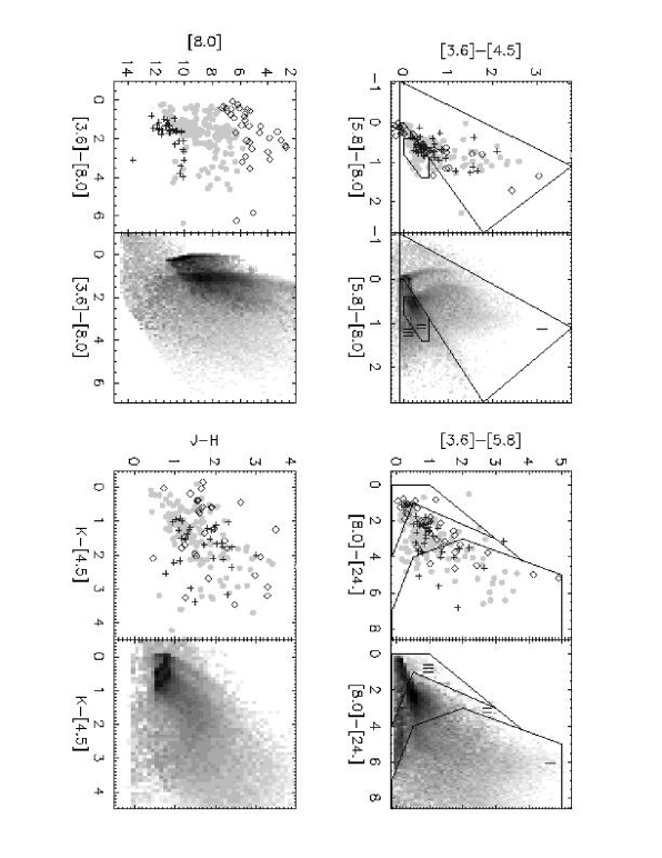
Figure 11: Color-color and color-magnitude plots of the 235 Serpens YSO’s compared with the distributions from models of Robitaille et al. (2007). The symbols are for the three different luminosity groups discussed in the text: open diamonds, L $>1$ L_⊙; light filled circles, 0.02 L_⊙$<L<1$ L_⊙; plus signs, L $<0.02$ L_⊙. The model data were those for their model cluster, with a distance of 260 pc for Serpens and with the c2d completeness limits. Also shown are the rough areas from Robitaille et al. (2007) occupied by mainly stage I, II, and III models.

8.2 Spectral Energy Distribution Modeling

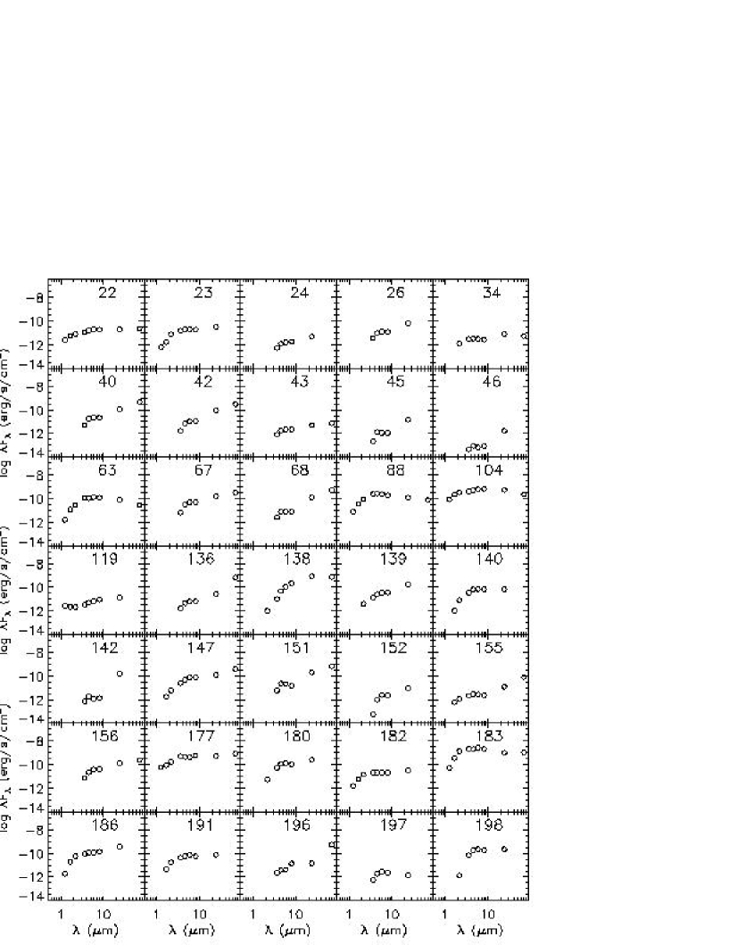
Figure 12: Spectral Energy Distributions of the Class I sources in the sample. The open dots signal the observed fluxes from J-band to MIPS-70 when available. The label gives the index in Table A.

In order to go beyond the general conclusions possible from color-color and color-magnitude plots, we have modelled the large fraction of our sources for which enough data are available to characterize them as likely star-plus-disk objects. For this analysis we have selected all Class II and Class III YSO’s. We expect these objects to have a reddened photosphere plus an infrared excess coming from the circumstellar material, most likely in a disk configuration. For completeness we show, without modeling, the SED’s of the remaining YSO’s. Figures 12 to 20 show the SEDs of all Class I, Class Flat, Class II and Class III sources. The open dots are the observed fluxes and generally include 2MASS J, H, and K fluxes followed by the four IRAC fluxes at 3.6, 4.5, 5.8 and 8.0 $\mu$m and by the MIPS fluxes at 24 and 70 $\mu$m when available. For the Class IIs and IIIs, we characterize the emission from the disk by comparing the energy distribution with that of a low-mass star. For this, we have computed the extinction from the J-K colors assuming a K7 underlying star, and then we have dereddened the observed fluxes with the interstellar extinction law of Weingartner & Draine (2001) with R${}_{v}=5.5$ to fit the dereddened SEDs to a NEXTGEN (Hauschildt et al. 1999) model of a K7 stellar photosphere. In the plots, the filled dots are the dereddened fluxes and the grey line is the photospheric emission from the star. Each SED is labeled with the identification number in Table A. The parameters of the model fits are listed in Tables A and A.

Two main assumptions are used in this approach. The first is that the star is a low-mass star; this is reasonable given the fact that the luminosity function discussed earlier peaks at $L\sim few\times 10^{-2}$L_⊙. In addition, Oliveira et al. (2007) have found that 30 of the 39 YSO’s they observed out of our sample had spectral types of K or M. The second assumption is that there is no substantial excess in the near infrared bands, where we consider all flux to be photospheric. This assumption is obviously only correct for those stars in the sample without strong on-going disk accretion. Cieza et al. (2005) have demonstrated that near-IR excesses as short as J-band can be seen in some actively accreting T Tauri stars, and they give an observed range of J-band excesses of 0.1 – 1.0 mag for their sample of sources in Taurus. The effect of this excess on the computed parameters implies that the stellar luminosities for the Class II objects are upper limits and therefore the disk luminosities are lower limits. More specifically, neglecting an excess flux in the J-band of 1.1 magnitude in one object would reduce its Ldisk/Lstar ratio by 12 % and modify the disk emission SED, diminishing its excess mostly at the shorter wavelengths. That would only happen, however, to the fraction of objects that are strongly accreting. Oliveira et al. (2007) found strong H-$\alpha$ emission indicative of active accretion in only 12 out of 39 Serpens YSO’s observed. We ran a test removing these objects from the final statistics and this did not change the overall picture.

The dashed line in the SED plots is the median SED of T Tauri stars in Taurus (Hartmann et al., 2005) normalized to the dereddened J-band flux of our SEDs. It represents the typical SED of an optically thick accreting disk around a Classical T Tauri star and is shown here to allow a qualitative estimation of the presence of disk evolution and dust settling. Based on similarity to this median SED, we define as T an SED which is identical to it, within the errors, as L, an SED with lower fluxes at some wavelengths, and H an object with larger fluxes than the median T Tauri SED. We have labeled the objects with these codes and use them to interpret the state of disk evolution. We interpret the L-type objects as thin disks which could perhaps result from dust grain growth and settling to the mid-plane, similar to the “anemic disks” in Lada et al. (2006). Objects 3 and 5 are good examples of T-type objects, numbers 11 and 18 are L-type stars, and number 8 is a H-type object. Also, we have labeled as LU objects that have photospheric fluxes up to around 8$\mu$m but then a sudden jump at longer wavelengths to the levels of a T-Tauri disk. We believe these objects may have large inner holes in their still optically thick disks; number 19 is one example of these.

Out of the 171 sources in the sample that are Class II or Class III, 44 (26 %) are T-type, so equivalent to a classical T Tauri star, 125 (73 %) are L-type, so show evidence of some degree of disk evolution, and finally 2 (1 %) show larger fluxes than the median SED of Taurus. This latter category is generally the result of imperfect fitting to the stellar photosphere due to lack of near-IR data and will not be considered further.

The numbers above indicate that there are many young stars in Serpens with disks that are virtually identical to those in Taurus. This points to a very similar origin of the disk structure across star forming regions. Within the uncertainties in our modeling process discussed above, however, we see a majority of L-type objects (73 %) in Serpens. This suggests that the disks in Serpens may be generally more evolved or flattened that those in Taurus. Also, interestingly the number of LU-type objects, or those with large inner holes, amounts to 14 (11 % of the L-type objects and only 6 % of the total YSO sample including Class I and F sources). This very small incidence indicates that either the process producing these large inner holes is a very fast transitional phase in the disk evolution or that only a small number of systems undergo that phase. We examine this issue below. In order to put firmer limits on these numbers it will be necessary to get optical spectral types for the stars and optical photometry in order to produce more accurate photosphere/disk/extinction models.

The SEDs also allow a rough study of the disk properties across the surveyed area. For this purpose we integrated the stellar and total fluxes to calculate a ratio between the stellar and the disk fluxes. The corresponding distribution is shown in Figure 21. Again, the solid line is the whole Class II and III sample and the dotted line corresponds to the T-type SEDs. To guide the eye, we have marked the approximate regimes of these ratios measured in debris disks (Ldisk/Lstar $<$ 0.02), passive disks (0.02 $<$ Ldisk/Lstar $<$ 0.08 Kenyon & Hartmann 1987), and accretion disks (Ldisk/Lstar $>$ 0.1), respectively. The figure illustrates well the large variety of disk evolutionary phases that we observe in Serpens, as well as the large majority of massive, accreting disks in the region.

In order to study the disk evolution in the cloud, there is need for a better characterization of the full sample with optical spectroscopy. That work is in progress and will be published elsewhere. Here we explore further the shapes of the SEDs to test another evolutionary diagnostic of the disk status. We have found that the more commonly used evolutionary metrics, e.g. spectral slope, $\alpha$, bolometric temperature, $T_{bol}$, or the Class system discussed earlier do not seem to capture the full range of phenomena apparent in our distribution of SED’s for young stellar objects. We, therefore, use $\alpha_{\rm excess}$ and $\lambda_{\rm excess}$, two new second-order SED parameters presented in Cieza et al. (2006) that will be discussed in more detail in a separate paper. In short, $\lambda_{\rm excess}$ is the last wavelength where the observed flux is photospheric and $\alpha_{\rm excess}$ is the slope computed as $dlog(\lambda F_{\lambda})/dlog(\lambda)$ starting from $\lambda_{\rm excess}$. The first parameter gives us an indication of how close the circumstellar matter is to the central object and the latter one a measure of how optically thick it is. Given the assumptions above for the fitting process, our values are upper limits for $\lambda_{\rm excess}$, and correspondingly lower limits for $\alpha_{\rm excess}$ for the Class IIs. We assume good stellar fits for the Class III sources.

Figure 22 shows both values for a sample of Classical T Tauri stars (CTTs) from Cieza et al. (2005), weak-lined T Tauri stars (wTTs) from Cieza et al. (2006), debris disks from Chen et al. (2005), and our sample of YSOs in Serpens. Cieza et al. (2006) found that $\lambda_{\rm excess}$ is well correlated with evolutionary phase and also, as seen in Figure 22, that $\alpha$ is observed over wider ranges for later evolutionary phases. This suggests a large range of possible evolutionary paths for circumstellar disks. Objects could either evolve to the lower right side of the diagram, which could be interpreted as a sign of dust grain growth and settling to the disk mid-plane; they could also move to the right and up, from creation of a large inner hole in their disks while retaining a massive outer disk, and also, as this diagram shows, all intermediate pathways in between both extremes.

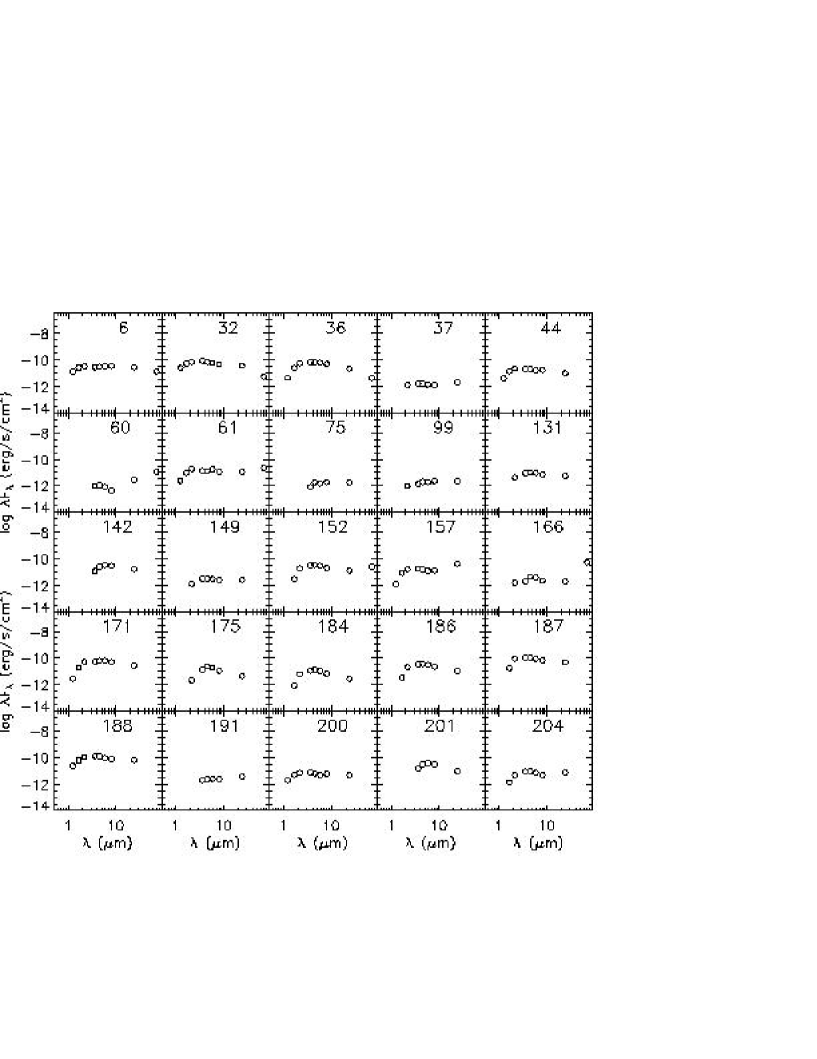
Figure 14: Spectral Energy Distributions of the Flat sources in the sample. Symbols as in Figure 12.

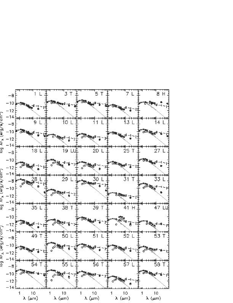
Figure 15: Spectral Energy Distributions (SED) of the Class II sources in the sample. The open and solid dots are the observed and dereddened fluxes respectively. The grey line is the stellar model of a K7 star and the dashed line is the median SED of the TTauri stars in Taurus by Hartmann et al. (2005) normalized to the dereddened J-band flux for comparison. See text for more information.

Figure 16: Spectral Energy Distributions of the Class II sources in the sample (continued).

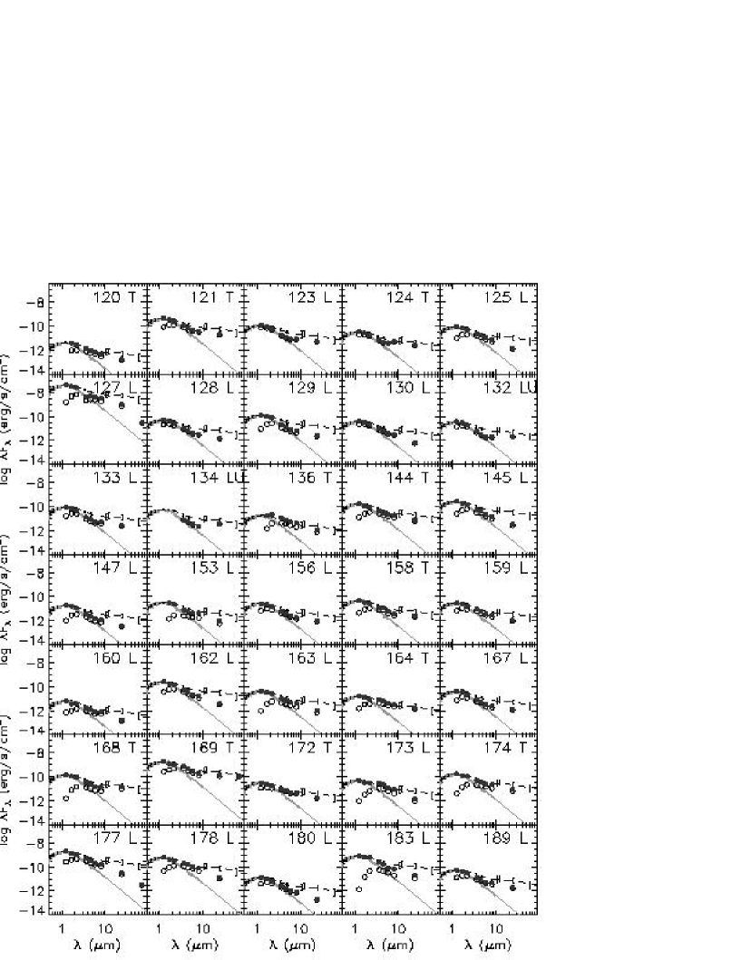
Figure 17: Spectral Energy Distributions of the Class II sources in the sample (continued).

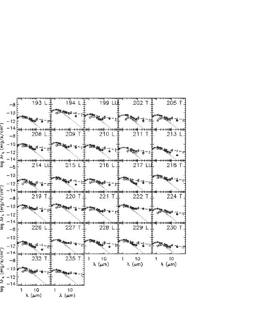
Figure 18: Spectral Energy Distributions of the Class II sources in the sample (continued).

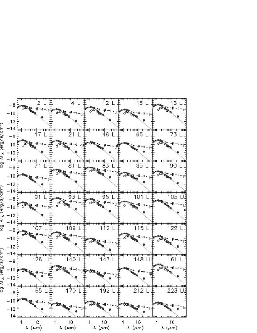
Figure 19: Spectral Energy Distributions of the Class III sources in the sample.

Figure 20: Spectral Energy Distributions of the Class III sources in the sample.

Figure 21: Distribution of disk to star luminosity ratios. The solid and dashed lines are the total sample and T Tauri-like sample of SEDs, respectively. Also marked are the typical ranges of L_disk/L_star ratios for debris disks, passive irradiated disks and accretion disks. The figure indicates that objects of all three evolutionary stages are found in Serpens, with a predominance of young accreting T Tauri-type stars.

Figure 22: Distribution of excess slopes $\alpha_{\rm excess}$ with respect to the wavelength at which the infrared excess begins $\lambda_{\rm turn-off}$ for the sample of wTTs (solid dots), a sample of cTTs in Lupus from Cieza et al. (2006), the median SED of cTTs in Taurus from D’Alessio et al. (1999) in asterisks (marked as D99), and a sample of debris disks from Chen et al. (2005) in diamonds. The arrows represent the limits for the class II objects in Serpens and the triangles the Class III sources. The diagram shows a much larger spread in inner disk morphologies in the more evolved objects than in the least evolved ones. The Serpens objects follow the previously observed trend.

9 Selected Sources

9.1 The Coldest Objects

Table A lists the 15 YSO’s that display the coldest energy distributions. These are the objects whose ratio of $F_{70}/F_{24}>8$. Six of these are in Cluster A (the core) and four in Cluster B. Two are in a small grouping about 0.2^∘ northeast of Cluster B, and the remaining three appear as isolated cold objects, though in areas with other moderately red objects. All of these except for two of the isolated cold objects, ID’s 105 and 148, are associated with dense clumps of millimeter emission as seen by Enoch et al. (2007). As discussed in the following section, two in Cluster A and one in Cluster B are associated with high velocity outflows. As has been noted already by Padgett et al. (2004) and Rebull et al. (2006), it is striking how many of these coldest, most obscured YSO’s are located in compact clusters together with objects that are substantially more evolved in the nominal system of classes, e.g. Class II and III.

9.2 Outflow Sources

A number of recent Spitzer studies have found that high-velocity shocked outflows from young stars are visible in IRAC images, typically strongest at 4.5$\mu$m (Noreiga-Crespo et al., 2004). We have examined our images for such outflows as well as for correspondance with the lists of published HH objects in the region (Ziener & Eisloffel, 1999). Table 10 summarizes the results of this effort. Two strong, obvious jet-like features are seen in Cluster A and one in Cluster B. In addition, as shown in Table 10, we find small extended features at the positions of most of the known HH objects in Serpens that were within our covered area. The two “jets” in Cluster A appear to originate from two of the most deeply embedded objects in this cluster that are associated with the sub-mm sources SMM1 and SMM5 (Testi & Sargent, 1998). Both these outflows are aligned roughly in the NW-SE direction and are visible on both sides of the central 24$\mu$m likely exciting sources. In Cluster B there is one obvious jet-like feature extending mostly south of YSO # 75. There is also probably faint emission visible 30^′′ to the north of the embedded source as well. Harvey et al. (2007) discuss the Cluster B jet and several nearby Spitzer sources in more detail. Figures 23 and 24 show 3-color images of Clusters A and B with the color tables chosen to make these jets most visible. In addition to the optical HH objects in the Serpens Clouds, there are a number of high-velocity molecular outflows that have been mapped in Cluster A (Davis et al., 1999). These maps present a confusing picture of outflows, and because of the relatively larger beamwidth of the mm observations and close packing of infrared sources in this cluster, it is very difficult to associate the radio outflows unequivocally with particular Spitzer sources.

Figure 23: Three-color image of the Cluster A area of Serpens. The color coding is: blue/4.5$\mu$m, green/8.0$\mu$m, and red/24$\mu$m. Some of the more obvious objects that are likely to be jets are marked by arrows. The region of the disappearing source 81 of Eiroa & Casali (1992) is circled.

Figure 24: Three-color image of the Cluster B area of Serpens as for Figure 23.

9.3 Other Objects

Horrobin, Casali & Eiroa (1997) reported on the disappearance of a bright near-infrared source in Serpens from the earlier study of EC92. Table A shows that we also see no obvious source at the position of EC92-81, other than a low S/N single-band detection of a source moderately distant from the nominal position. Interestingly, though, this area marked in Figure 23 appears to contain several small knots of emission that may represent shocked gas. For example, there are two small knots visible in our 4.5 and 8.0$\mu$m images that have no 3.6 or 24$\mu$m counterparts (and therefore not classified as YSO’s). These two knots at RA = 18 29 56.7, Dec = +01 13 19 (J2000), are only 12^′′ south of the position of EC92-81. Therefore it is possible that the original source was a small clump of excited gas that has moved or dissipated since the original study of EC92, and perhaps, these Spitzer knots are related to that earlier source in some way.

10 Overall Results on Star Formation

The overall picture of star formation in Serpens is summarized in Table 6. As noted earlier, the surface density of young stars is much higher in Clusters A and B than in the rest of the cloud, by factors of 10 to 20. On the other hand, the majority of YSOs (74%) are not in the clusters, but in the rest of the cloud. If we assume a mean mass for the stars of 0.5 M_⊙ and assume that star formation has been proceeding for 2 Myr, we can estimate the rate at which the clusters and the whole cloud are converting mass into stars. These values are also given in Table 6. The Serpens cloud that we have surveyed is turning nearly 60 M_⊙ into stars per Myr. The rates for the clusters are probably underestimates because they are probably younger than 2 Myr, a typical duration for the Class II SED. Of course, a significant number of the older objects outside the clusters may have, in fact, formed in these or earlier clusters. A 1 km s^-1 random motion of a YSO relative to its birthplace results in 1 pc of movement in 10⁶ yr, or nearly 1/4 degree at the distance of Serpens.

The distribution of YSOs over class supports the younger age for the clusters than for star formation in general in Serpens. While the ratio of the number of Class I and Flat spectrum sources to the number of Class II and Class III sources is 0.37 for the whole cloud, similar to other clouds surveyed by c2d (Evans et al., in prep.), the same ratio is 3.0 for Cluster A and 1.4 for Cluster B. These high ratios strongly suggest that Cluster A is too young for most YSOs to have reached the Class II stage. In contrast, this ratio is 0.14 for the rest of the cloud, outside the clusters, which is strongly dominated by Class II and Class III objects.

11 Summary

We have identified a high-confidence set of 235 YSO’s in Serpens by a set of criteria based on comparison with data from the Spitzer SWIRE Legacy program. This is a large enough number that we can draw important statistical conclusions about various properties of this set. If we assume that the “Class System” of Lada (1987) and Greene et al. (1994) represents an evolutionary sequence, then the relative numbers of YSO’s found in each of the first three classes (I, flat, and II) suggests that the Class II phase lasts substantially longer than the combined total of the Class I and “Flat” phases, based on the overall cloud statistics. The clusters, however, show more YSOs in the Class I and Flat phases than in Class II, indicating that they are very young. The majority of YSOs (mostly Class II) are outside the clusters and probably represent a somewhat older epoch of star formation compared to the intense star formation now going on in the clusters. The surface density of YSOs in the clusters exceeds that of the rest of the cloud by factors of 10 to 20 (Table 6).

The luminosity function for the Serpens YSO’s is populated down to luminosities of $3\times 10^{-3}$ L_⊙. It may extend even lower, but our ability to distinguish low luminosity YSO’s is severely restricted by the large population of background galaxies at these flux levels. The lower luminosity YSO’s, $L<2\times 10^{-2}$ L_⊙, exhibit a similar spatial distribution and SED slope distribution to those of their higher luminosity counterparts. This is consistent with the conclusion that they have formed in similar ways.

12 Acknowledgments

Support for this work, part of the Spitzer Legacy Science Program, was provided by NASA through contracts 1224608, 1230782, and 1230779 issued by the Jet Propulsion Laboratory, California Institute of Technology, under NASA contract 1407. Astrochemistry in Leiden is supported by a NWO Spinoza grant and a NOVA grant. B.M. thanks the Fundación Ramón Areces for financial support. This publication makes use of data products from the Two Micron All Sky Survey, which is a joint project of the University of Massachusetts and the Infrared Processing and Analysis Center/California Institute of Technology, funded by NASA and the National Science Foundation. We also acknowledge extensive use of the SIMBAD data base.

Appendix A YSO Selection Process

The procedure we use to select YSO’s and de-select extra-galactic background sources is based on the color-magnitude diagrams shown in Figure 3. We construct “probability” functions for each of the three color-magnitude diagrams based on where a source falls relative to the black dashed lines in each diagram. These three “probabilities” are multiplied and then additional adjustments to the probability are made based on several additional properties of the source fluxes and whether or not they were found to be larger than point-like in the source extraction process.

In the [4.5] vs. [4.5]-[8.0] color magnitude diagram, the probability function is:

$$P_{i2i4}=0.7\times\{1-exp(-[1.2+0.5(M_{4.5}-D)]^{3})\}$$

where:

$$D = 13.05\mbox{ for }M_{4.5}-M_{8.0}>1.4$$

$$= 14.5\mbox{ for }0.5\geq M_{4.5}-M_{8.0}<1.4\mbox{ and object was found to be pointlike in all IRAC bands}$$

$$= 12.5\mbox{ for }0.5\geq M_{4.5}-M_{8.0}<1.4\mbox{ and object was found to be extended at 3.6 or 4.5$\mu$m}$$

$$= 14.5\mbox{ for }M_{4.5}-M_{8.0}<0.5$$

In the [24] vs. [8.0]-[24] color magnitude diagram, the probability function is:

$$P_{i4m1}=exp(-\{[(M_{8}-M_{24}-3.5)/1.7]^{2}+[(M_{24}-9)/2)^{2}\}$$

and $P_{i4-m1}$ is set to a minimum of 0.1.

In the [24] vs. [4.5]-[8.0] color magnitude diagram, the probability function is:

$$P_{i24m1}=0.7\times\{1-exp(-[M_{4.5}-M_{8}+0.8-(10-M_{24})/1.8\}$$

and $P_{i24m1}$ is set to a minimum of 0.

The combined “probability” is then:

$$P_{tot}=P_{i2i4}\times P_{i4m1}\times P_{i24m1}$$

Additionally, the following factors influence modifications to $P_{tot}$:

$$P_{tot} / (K-[4.5])$$

$$P_{tot} \times 2\mbox{ for sources that are extended at 3.6 or 4.5$\mu$m}$$

$$P_{tot} = 0.1\mbox{ where [24] $>$ 10 (i.e. assumed GALc)}$$

$$P_{tot} \times 0.1\mbox{ where $F_{70}>$ 400 mJy and source detected at 5.8,8, and 24$\mu$m}$$

Based on the distribution of $P_{tot}$ shown in Figure 4, we chose the dividing line between YSO’s and extra-galactic sources to be $log_{10}(P_{tot})=-1.47$.

Table 1: YSO vs. X-Gal Discrimination Criteria

Criterion	Contaminant Probability
K - [4.5]	Prob$/(K-[4.5])$
[4.5] (for [4.5]-[8.0] $<$ 0.5)	Smooth increase for [4.5] $>$ 14.5
[4.5] (for 0.5 $<$ [4.5]-[8.0] $<$ 1.4, Extended)	Smooth increase for [4.5] $>$ 12.5
[4.5] (for 0.5 $<$ [4.5]-[8.0] $<$ 1.4, Pointlike)	Smooth increase for [4.5] $>$ 14.5
[4.5] (for 1.4 $<$ [4.5]-[8.0])	Smooth increase for [4.5] $>$ 13.0
$([8.0]-[24]-3.5)^{2}/1.7+([24]-9.0)^{2}/2$	Smooth increase for values $<$ 1
$[4.5]-[8.0]-0.55(10.-[24])$	Smooth increase for values $>$ 1
[24] (for all colors)	100% probability for [24] $>$ 10.0
Extended at 3.6 or 4.5$\mu$m	Twice as likely to be X-gal
$F_{70}$	X-gal prob $\times$ 0.1 for $F_{70}>$ 400 mJy

Table 2: YSO’s in Serpens

ID	Name/Position	Prev. Name	3.6 $\mu$m	4.5 $\mu$m	5.8 $\mu$m	8.0 $\mu$m	24.0 $\mu$m	70.0 $\mu$m
	SSTc2dJ…		(mJy)	(mJy)	(mJy)	(mJy)	(mJy)	(mJy)
1	18275381$-$0002333		25.5$\pm$ 1.2	20.2$\pm$ 1.0	15.6$\pm$ 0.7	13.9$\pm$ 0.7	22.7$\pm$ 2.1	$\cdots$
2	18280503$+$0006593		783$\pm$ 55	426$\pm$ 29	358$\pm$ 18	218$\pm$ 14	76.4$\pm$ 7.1	$\cdots$
3	18280845$-$0001064		140$\pm$ 7	108$\pm$ 8	129$\pm$ 6	122$\pm$ 8	161$\pm$ 14	314$\pm$ 36
4	18281100$-$0001393		104$\pm$ 5	63.4$\pm$ 3.2	54.6$\pm$ 2.6	35.4$\pm$ 1.9	9.51$\pm$0.90	$\cdots$
5	18281350$-$0002491	CDF88-2	105$\pm$ 5	88.1$\pm$ 4.7	77.5$\pm$ 3.7	94.3$\pm$ 5.0	254$\pm$ 23	382$\pm$ 43
6	18281501$-$0002588		33.3$\pm$ 1.6	45.6$\pm$ 2.3	61.5$\pm$ 3.1	96.3$\pm$ 5.8	225$\pm$ 20	320$\pm$ 41
7	18281519$-$0001405		7.18$\pm$0.35	6.18$\pm$0.30	5.15$\pm$0.25	5.01$\pm$0.26	8.00$\pm$0.77	$\cdots$
8	18281525$-$0002432	CoKu Ser-G1	174$\pm$ 9	177$\pm$ 9	180$\pm$ 11	191$\pm$ 11	1200$\pm$ 25	1670$\pm$ 169
9	18281628$-$0003161		53.1$\pm$ 2.7	48.4$\pm$ 2.4	45.4$\pm$ 2.1	46.2$\pm$ 2.5	74.7$\pm$ 6.9	129$\pm$ 24
10	18281852$-$0003329		3.38$\pm$0.17	3.14$\pm$0.15	3.13$\pm$0.16	2.99$\pm$0.15	2.96$\pm$0.36	$\cdots$
11	18281981$-$0001474		5.52$\pm$0.27	5.28$\pm$0.26	4.90$\pm$0.24	4.02$\pm$0.21	5.58$\pm$0.54	$\cdots$
12	18282010$+$0029145		237$\pm$ 21	109$\pm$ 9	116$\pm$ 8	76.6$\pm$ 4.8	17.5$\pm$ 1.6	$\cdots$
13	18282143$+$0010411		13.7$\pm$ 0.7	10.1$\pm$ 0.6	9.99$\pm$0.49	8.90$\pm$0.50	10.5$\pm$ 1.0	$\cdots$
14	18282158$+$0000164		60.3$\pm$ 3.0	54.0$\pm$ 2.8	45.5$\pm$ 2.2	61.4$\pm$ 3.4	170$\pm$ 15	126$\pm$ 21
15	18282432$+$0034545	D-002	62.4$\pm$ 4.2	46.1$\pm$ 3.0	41.1$\pm$ 2.5	32.5$\pm$ 2.0	13.9$\pm$ 1.3	$\cdots$
16	18282738$-$0011499		1130$\pm$ 60	660$\pm$ 35	631$\pm$ 30	399$\pm$ 22	120$\pm$ 11	$\cdots$
17	18282740$+$0000239		87.3$\pm$ 4.5	54.6$\pm$ 2.7	47.3$\pm$ 2.2	32.3$\pm$ 1.6	12.9$\pm$ 1.2	$\cdots$
18	18282849$+$0026500		2.47$\pm$0.16	2.28$\pm$0.15	2.27$\pm$0.15	2.52$\pm$0.16	2.62$\pm$0.37	$\cdots$
19	18282905$+$0027561	D-007	9.80$\pm$0.57	8.51$\pm$0.47	7.03$\pm$0.38	5.46$\pm$0.30	43.4$\pm$ 4.0	$\cdots$
20	18284025$+$0016173		3.71$\pm$0.20	3.86$\pm$0.20	3.60$\pm$0.19	3.59$\pm$0.18	2.89$\pm$0.35	$\cdots$
21	18284052$+$0022145		68.2$\pm$ 3.7	41.2$\pm$ 2.4	39.2$\pm$ 2.0	25.5$\pm$ 1.4	11.7$\pm$ 1.1	$\cdots$
22	18284186$-$0003213		13.7$\pm$ 0.7	24.8$\pm$ 1.2	39.6$\pm$ 1.9	49.0$\pm$ 2.6	155$\pm$ 14	538$\pm$ 54
23	18284400$+$0053379		18.1$\pm$ 0.9	29.7$\pm$ 1.4	40.3$\pm$ 2.0	49.9$\pm$ 2.5	260$\pm$ 24	$\cdots$
24	18284477$+$0051257		0.65$\pm$0.04	1.77$\pm$0.09	3.08$\pm$0.16	4.81$\pm$0.23	37.6$\pm$ 3.5	$\cdots$
25	18284481$+$0048085		7.80$\pm$0.40	7.30$\pm$0.36	5.68$\pm$0.28	6.68$\pm$0.33	10.0$\pm$ 0.9	$\cdots$
26	18284496$+$0052035	IRAS 18262+0050	4.32$\pm$0.28	14.2$\pm$ 0.8	25.6$\pm$ 1.3	31.5$\pm$ 2.0	547$\pm$ 11	$\cdots$
27	18284497$+$0045239		41.3$\pm$ 2.1	33.7$\pm$ 1.6	31.3$\pm$ 1.5	30.7$\pm$ 1.6	20.8$\pm$ 1.9	$\cdots$
28	18284558$-$0007127	IRAS 18261-0009	2920$\pm$ 182	2790$\pm$ 172	3070$\pm$ 155	2990$\pm$ 222	2150$\pm$ 200	206$\pm$ 23
29	18284613$+$0003016		8.40$\pm$0.45	9.41$\pm$0.47	9.80$\pm$0.47	10.5$\pm$ 0.6	7.95$\pm$0.76	$\cdots$
30	18284784$+$0008402	VV Ser	2460$\pm$ 176	2530$\pm$ 180	3430$\pm$ 256	3830$\pm$ 271	2970$\pm$ 281	600$\pm$ 59
31	18284808$+$0019266		2.37$\pm$0.14	2.68$\pm$0.15	2.42$\pm$0.14	2.57$\pm$0.14	2.50$\pm$0.36	$\cdots$
32	18285020$+$0009497		105$\pm$ 5	107$\pm$ 6	113$\pm$ 5	121$\pm$ 6	291$\pm$ 27	129$\pm$ 28
33	18285038$-$0012550		322$\pm$ 17	252$\pm$ 12	232$\pm$ 12	170$\pm$ 9	62.3$\pm$ 5.8	$\cdots$
34	18285122$+$0019273		3.47$\pm$0.18	5.12$\pm$0.26	5.81$\pm$0.29	7.42$\pm$0.39	65.4$\pm$ 6.1	130$\pm$ 16
35	18285200$+$0015516		1.65$\pm$0.09	1.60$\pm$0.08	1.30$\pm$0.08	1.58$\pm$0.09	1.31$\pm$0.22	$\cdots$
36	18285249$+$0020260		81.4$\pm$ 4.7	95.7$\pm$ 5.8	115$\pm$ 5	129$\pm$ 7	177$\pm$ 16	102$\pm$ 19
37	18285276$+$0028467	D-060	1.84$\pm$0.10	2.45$\pm$0.14	2.58$\pm$0.15	3.44$\pm$0.19	15.7$\pm$ 1.5	$\cdots$
38	18285364$+$0019409		3.56$\pm$0.19	4.34$\pm$0.24	4.03$\pm$0.21	3.72$\pm$0.20	5.56$\pm$0.56	$\cdots$
39	18285395$+$0045530		12.5$\pm$ 0.6	10.5$\pm$ 0.5	9.45$\pm$0.46	11.2$\pm$ 0.6	25.4$\pm$ 2.4	$\cdots$
40	18285404$+$0029299	D-062/D-066	5.81$\pm$0.50	27.6$\pm$ 2.3	44.8$\pm$ 2.6	56.4$\pm$ 3.2	918$\pm$ 85	11100$\pm$ 1040
41	18285450$+$0028523	D-064	14.7$\pm$ 0.9	34.2$\pm$ 2.0	44.8$\pm$ 2.3	25.4$\pm$ 1.4	4.53$\pm$0.48	$\cdots$
42	18285486$+$0029525	D-065	1.94$\pm$0.12	10.6$\pm$ 0.6	20.4$\pm$ 1.1	30.2$\pm$ 1.6	765$\pm$ 70	7250$\pm$ 675
43	18285489$+$0018326		0.95$\pm$0.05	2.54$\pm$0.15	4.24$\pm$0.23	5.88$\pm$0.32	39.4$\pm$ 3.7	179$\pm$ 23
44	18285529$+$0020522		24.5$\pm$ 1.3	29.1$\pm$ 1.7	32.7$\pm$ 1.7	47.2$\pm$ 2.6	75.6$\pm$ 7.0	$\cdots$
45	18285577$+$0029447	IRAS 18263+0027	0.26$\pm$0.02	1.87$\pm$0.14	2.23$\pm$0.14	3.08$\pm$0.17	126$\pm$ 11	$\cdots$
46	18285664$+$0030082		0.055$\pm$0.007	0.14$\pm$0.01	0.12$\pm$0.03	0.22$\pm$0.05	13.0$\pm$ 1.2	$\cdots$
47	18285715$+$0048360		1.55$\pm$0.08	1.38$\pm$0.07	1.18$\pm$0.07	0.74$\pm$0.06	8.83$\pm$0.83	$\cdots$
48	18285808$+$0017244		52.5$\pm$ 3.0	36.7$\pm$ 2.5	31.2$\pm$ 1.7	28.5$\pm$ 1.7	9.74$\pm$0.92	1040$\pm$ 101
49	18285860$+$0048594		10.8$\pm$ 0.5	9.32$\pm$0.48	7.40$\pm$0.35	7.25$\pm$0.43	13.4$\pm$ 1.2	$\cdots$
50	18285945$+$0030031	D-074	38.4$\pm$ 2.1	41.0$\pm$ 2.2	43.5$\pm$ 2.3	49.4$\pm$ 2.7	81.6$\pm$ 7.6	204$\pm$ 32
51	18290025$+$0016580		44.4$\pm$ 2.5	34.2$\pm$ 2.2	33.2$\pm$ 1.7	33.4$\pm$ 1.8	39.2$\pm$ 3.6	$\cdots$
52	18290057$+$0045079		17.2$\pm$ 0.8	17.0$\pm$ 0.8	13.4$\pm$ 0.6	13.0$\pm$ 0.6	23.6$\pm$ 2.2	$\cdots$
53	18290082$+$0027468	D-080	8.81$\pm$0.52	9.62$\pm$0.55	10.5$\pm$ 0.6	13.2$\pm$ 0.7	29.0$\pm$ 2.7	$\cdots$
54	18290089$+$0029316	D-078	246$\pm$ 13	290$\pm$ 16	308$\pm$ 19	392$\pm$ 23	711$\pm$ 67	736$\pm$ 75
55	18290107$+$0031452	D-081	59.2$\pm$ 3.6	72.8$\pm$ 4.3	76.2$\pm$ 4.1	75.5$\pm$ 4.3	72.5$\pm$ 6.7	$\cdots$
56	18290122$+$0029330	CoKu Ser-G6	88.8$\pm$ 4.8	97.4$\pm$ 5.1	91.0$\pm$ 5.3	100$\pm$ 6	215$\pm$ 21	$\cdots$
57	18290153$+$0017299		3.16$\pm$0.18	2.69$\pm$0.17	2.92$\pm$0.16	2.43$\pm$0.14	1.43$\pm$0.26	$\cdots$
58	18290175$+$0029465	CoKu Ser-G4	141$\pm$ 8	133$\pm$ 6	111$\pm$ 6	107$\pm$ 10	361$\pm$ 33	$\cdots$
59	18290184$+$0029546	CoKu Ser-G3	586$\pm$ 51	553$\pm$ 33	504$\pm$ 28	461$\pm$ 27	407$\pm$ 38	503$\pm$ 52
60	18290211$+$0031206		1.19$\pm$0.07	1.62$\pm$0.09	1.58$\pm$0.10	1.13$\pm$0.07	22.1$\pm$ 2.0	276$\pm$ 29
61	18290283$+$0030095	D-084	15.4$\pm$ 1.0	19.2$\pm$ 1.1	34.5$\pm$ 2.0	30.6$\pm$ 1.8	94.2$\pm$ 8.7	535$\pm$ 54
62	18290393$+$0020217		182$\pm$ 10	175$\pm$ 11	179$\pm$ 9	171$\pm$ 12	255$\pm$ 23	283$\pm$ 30
63	18290437$+$0033240	D-086	133$\pm$ 7	165$\pm$ 12	256$\pm$ 13	300$\pm$ 18	615$\pm$ 57	651$\pm$ 67
64	18290517$+$0038439		3.43$\pm$0.23	4.04$\pm$0.20	2.52$\pm$0.16	2.04$\pm$0.11	6.73$\pm$0.64	$\cdots$
65	18290575$+$0022325		36.3$\pm$ 2.2	27.1$\pm$ 1.5	17.8$\pm$ 1.0	13.6$\pm$ 0.7	15.1$\pm$ 1.4	$\cdots$
66	18290615$+$0019444		7.24$\pm$0.40	5.80$\pm$0.31	4.70$\pm$0.25	4.90$\pm$0.26	10.3$\pm$ 1.0	$\cdots$
67	18290619$+$0030432	IRAS 18265+0028?	8.05$\pm$0.41	45.0$\pm$ 2.8	93.9$\pm$ 4.8	129$\pm$ 7	1320$\pm$ 139	7240$\pm$ 713
68	18290675$+$0030343	IRAS 18265+0028?	3.27$\pm$0.21	11.7$\pm$ 0.7	14.9$\pm$ 0.8	20.7$\pm$ 1.2	1000$\pm$ 105	11400$\pm$ 1180
69	18290697$+$0038380	D-096	21.3$\pm$ 1.4	29.3$\pm$ 1.5	22.5$\pm$ 1.3	22.7$\pm$ 1.1	40.2$\pm$ 3.7	$\cdots$
70	18290741$+$0019215		3.07$\pm$0.17	2.28$\pm$0.13	2.17$\pm$0.12	1.71$\pm$0.09	0.93$\pm$0.19	$\cdots$
71	18290763$+$0052223		4.50$\pm$0.23	4.03$\pm$0.20	3.59$\pm$0.18	4.66$\pm$0.23	9.58$\pm$0.89	$\cdots$
72	18290775$+$0054037		10.2$\pm$ 0.5	9.86$\pm$0.48	9.66$\pm$0.47	10.2$\pm$ 0.5	11.0$\pm$ 1.0	$\cdots$
73	18290808$-$0007371		121$\pm$ 6	71.5$\pm$ 3.6	61.1$\pm$ 2.9	38.8$\pm$ 2.1	9.83$\pm$0.92	$\cdots$
74	18290817$+$0105445		31.2$\pm$ 1.6	20.7$\pm$ 1.0	14.1$\pm$ 0.7	9.66$\pm$0.47	6.58$\pm$0.63	$\cdots$
75	18290904$+$0031280		0.95$\pm$0.11	2.78$\pm$0.23	2.92$\pm$0.24	5.03$\pm$0.40	14.0$\pm$ 1.9	$\cdots$
76	18290955$+$0037020	IRAS 18266+0035	837$\pm$ 66	784$\pm$ 48	873$\pm$ 61	904$\pm$ 46	531$\pm$ 49	85.6$\pm$20.2
77	18290980$+$0034459	D-105	1260$\pm$ 70	1060$\pm$ 72	1070$\pm$ 72	1000$\pm$ 52	778$\pm$ 72	76.8$\pm$13.1
78	18291148$+$0020387		4.46$\pm$0.27	3.36$\pm$0.19	2.39$\pm$0.15	1.72$\pm$0.10	16.0$\pm$ 1.5	$\cdots$
79	18291249$+$0018150		5.46$\pm$0.31	5.15$\pm$0.29	4.26$\pm$0.25	4.22$\pm$0.21	6.49$\pm$0.67	$\cdots$
80	18291288$+$0009477		2.60$\pm$0.13	2.02$\pm$0.11	1.98$\pm$0.11	2.14$\pm$0.11	2.18$\pm$0.31	$\cdots$
81	18291407$+$0002589		313$\pm$ 16	197$\pm$ 10	170$\pm$ 8	104$\pm$ 5	30.7$\pm$ 2.9	$\cdots$
82	18291432$+$0107300		2.98$\pm$0.16	2.56$\pm$0.13	2.29$\pm$0.12	2.15$\pm$0.11	1.94$\pm$0.24	$\cdots$
83	18291508$+$0052124	IRAS 18266+0050	1210$\pm$ 64	663$\pm$ 36	616$\pm$ 31	468$\pm$ 24	295$\pm$ 27	$\cdots$
84	18291513$+$0039378		35.4$\pm$ 2.4	37.7$\pm$ 1.8	30.8$\pm$ 1.8	25.9$\pm$ 1.3	5.44$\pm$0.52	$\cdots$
85	18291539$-$0012519		73.1$\pm$ 3.7	52.1$\pm$ 2.5	44.3$\pm$ 2.1	42.1$\pm$ 2.3	25.2$\pm$ 2.3	$\cdots$
86	18291557$+$0039119		13.6$\pm$ 0.9	16.2$\pm$ 0.8	15.1$\pm$ 0.9	25.6$\pm$ 1.3	60.5$\pm$ 5.6	$\cdots$
87	18291562$+$0039230		6.42$\pm$0.46	7.33$\pm$0.35	5.99$\pm$0.35	8.05$\pm$0.39	32.5$\pm$ 3.0	135$\pm$ 15
88	18291617$+$0018227	IRAS 18267+0016	284$\pm$ 27	412$\pm$ 33	446$\pm$ 27	478$\pm$ 24	943$\pm$ 88	1740$\pm$ 165
89	18291969$+$0018031		19.6$\pm$ 1.3	20.0$\pm$ 1.1	16.4$\pm$ 0.9	18.0$\pm$ 0.9	31.8$\pm$ 3.0	$\cdots$
90	18292001$+$0024497	D-132	146$\pm$ 8	96.0$\pm$ 5.3	83.6$\pm$ 4.3	56.8$\pm$ 2.9	16.0$\pm$ 1.5	$\cdots$
91	18292003$+$0121015	K-112	126$\pm$ 6	73.9$\pm$ 3.7	61.5$\pm$ 2.9	38.6$\pm$ 2.0	9.95$\pm$0.95	$\cdots$
92	18292042$+$0121037		48.9$\pm$ 2.4	40.5$\pm$ 2.0	33.0$\pm$ 1.6	27.1$\pm$ 1.4	25.5$\pm$ 2.4	$\cdots$
93	18292095$+$0030346	D-137	911$\pm$ 60	414$\pm$ 36	511$\pm$ 31	377$\pm$ 20	187$\pm$ 17	$\cdots$
94	18292184$+$0019386		11.8$\pm$ 0.7	11.2$\pm$ 0.6	10.6$\pm$ 0.6	10.8$\pm$ 0.6	14.4$\pm$ 1.4	$\cdots$
95	18292616$+$0020518		742$\pm$ 55	377$\pm$ 26	382$\pm$ 28	245$\pm$ 14	84.6$\pm$ 7.8	$\cdots$
96	18292640$+$0030043		3.89$\pm$0.31	3.36$\pm$0.20	3.42$\pm$0.18	3.87$\pm$0.21	8.75$\pm$0.82	$\cdots$
97	18292678$+$0039498		9.98$\pm$0.73	13.3$\pm$ 0.6	9.40$\pm$0.62	11.9$\pm$ 0.6	34.5$\pm$ 3.2	64.9$\pm$11.5
98	18292729$+$0039066		2.18$\pm$0.15	3.08$\pm$0.15	2.29$\pm$0.16	2.37$\pm$0.12	1.73$\pm$0.22	$\cdots$
99	18292735$+$0038497		1.56$\pm$0.11	2.95$\pm$0.14	3.65$\pm$0.24	6.25$\pm$0.30	18.4$\pm$ 1.7	$\cdots$
100	18292822$-$0022571	IRAS 18268-0025	1280$\pm$ 76	1300$\pm$ 74	1550$\pm$ 104	1760$\pm$ 116	414$\pm$ 85	730$\pm$ 85
101	18292897$+$0013104		308$\pm$ 21	186$\pm$ 14	196$\pm$ 10	139$\pm$ 7	39.8$\pm$ 3.7	$\cdots$
102	18292927$+$0018000		7.00$\pm$0.37	5.90$\pm$0.34	5.35$\pm$0.27	5.31$\pm$0.28	4.51$\pm$0.44	$\cdots$
103	18293083$+$0101072	K-150	38.8$\pm$ 1.9	35.2$\pm$ 1.8	27.6$\pm$ 1.3	30.7$\pm$ 1.6	54.3$\pm$ 5.0	$\cdots$
104	18293195$+$0118429	K-159	481$\pm$ 24	786$\pm$ 42	1140$\pm$ 57	1830$\pm$ 138	4370$\pm$ 407	5190$\pm$ 501
105	18293254$-$0013233	CDF88-4	654$\pm$ 39	370$\pm$ 19	276$\pm$ 13	156$\pm$ 8	39.7$\pm$ 3.7	429$\pm$ 47
106	18293300$+$0040089		6.05$\pm$0.43	6.64$\pm$0.32	4.70$\pm$0.31	5.53$\pm$0.27	9.71$\pm$0.91	$\cdots$
107	18293319$+$0012122		687$\pm$ 37	445$\pm$ 30	469$\pm$ 22	339$\pm$ 17	86.7$\pm$ 8.0	$\cdots$
108	18293336$+$0108245	K-173	85.6$\pm$ 4.9	72.3$\pm$ 4.1	75.6$\pm$ 3.6	116$\pm$ 6	148$\pm$ 13	320$\pm$ 37
109	18293381$+$0053118		278$\pm$ 14	163$\pm$ 8	138$\pm$ 6	85.0$\pm$ 4.3	25.9$\pm$ 2.4	$\cdots$
110	18293561$+$0035038	D-176	30.5$\pm$ 2.0	24.1$\pm$ 1.4	17.0$\pm$ 1.0	12.8$\pm$ 0.7	74.2$\pm$ 6.9	57.6$\pm$13.1
111	18293619$+$0042167		21.1$\pm$ 1.2	19.9$\pm$ 1.0	15.6$\pm$ 0.8	12.8$\pm$ 0.6	81.1$\pm$ 7.5	126$\pm$ 17
112	18293635$+$0033560		8.01$\pm$0.52	5.68$\pm$0.33	4.54$\pm$0.27	2.90$\pm$0.15	1.25$\pm$0.18	$\cdots$
113	18293644$+$0046217		1.59$\pm$0.08	1.48$\pm$0.07	1.37$\pm$0.08	1.49$\pm$0.08	1.27$\pm$0.19	$\cdots$
114	18293670$+$0047579		17.3$\pm$ 0.8	15.7$\pm$ 0.8	12.4$\pm$ 0.6	11.9$\pm$ 0.6	17.3$\pm$ 1.6	$\cdots$
115	18293767$+$0111299	K-190	156$\pm$ 8	103$\pm$ 5	84.2$\pm$ 4.0	56.3$\pm$ 2.9	21.4$\pm$ 2.0	$\cdots$
116	18293881$+$0044381		4.99$\pm$0.25	4.58$\pm$0.22	3.93$\pm$0.19	3.72$\pm$0.19	3.35$\pm$0.34	$\cdots$
117	18293986$+$0117561	K-202	11.9$\pm$ 0.6	10.5$\pm$ 0.5	9.98$\pm$0.49	11.7$\pm$ 0.6	18.4$\pm$ 1.7	$\cdots$
118	18294020$+$0015131		3.93$\pm$0.22	7.40$\pm$0.41	13.4$\pm$ 0.7	24.4$\pm$ 1.3	113$\pm$ 10	126$\pm$ 15
119	18294121$+$0049020		7.47$\pm$0.37	6.04$\pm$0.29	5.67$\pm$0.28	7.37$\pm$0.35	7.54$\pm$0.71	$\cdots$
120	18294124$+$0047296		0.96$\pm$0.05	0.93$\pm$0.05	0.88$\pm$0.06	0.84$\pm$0.06	1.17$\pm$0.17	$\cdots$
121	18294146$+$0107380	K-207	95.4$\pm$ 4.8	83.2$\pm$ 4.1	72.2$\pm$ 3.4	81.0$\pm$ 4.3	147$\pm$ 13	$\cdots$
122	18294152$+$0110043	K-210	33.2$\pm$ 1.6	21.2$\pm$ 1.0	16.5$\pm$ 0.8	11.0$\pm$ 0.6	7.69$\pm$0.75	$\cdots$
123	18294168$+$0044270		20.6$\pm$ 1.0	16.5$\pm$ 0.8	14.9$\pm$ 0.7	20.1$\pm$ 1.0	40.0$\pm$ 3.7	$\cdots$
124	18294216$+$0120211	K-216	7.27$\pm$0.42	6.13$\pm$0.30	7.00$\pm$0.35	13.0$\pm$ 0.6	19.9$\pm$ 1.9	$\cdots$
125	18294392$+$0107208	K-219	18.4$\pm$ 0.9	17.8$\pm$ 0.9	16.1$\pm$ 0.8	13.3$\pm$ 0.6	10.1$\pm$ 1.0	$\cdots$
126	18294410$+$0033561		20.8$\pm$ 1.2	13.7$\pm$ 0.7	11.0$\pm$ 0.6	6.97$\pm$0.34	19.7$\pm$ 1.8	140$\pm$ 17
127	18294430$+$0104534	IRAS 18271+0102	2530$\pm$ 276	3920$\pm$ 263	5010$\pm$ 272	5040$\pm$ 401	5840$\pm$ 1750	655$\pm$ 65
128	18294452$+$0113115	EC-11	9.59$\pm$0.46	7.78$\pm$0.38	6.62$\pm$0.32	7.86$\pm$0.38	10.8$\pm$ 1.0	$\cdots$
129	18294503$+$0035266		13.9$\pm$ 0.8	12.5$\pm$ 0.7	10.8$\pm$ 0.6	11.2$\pm$ 0.6	16.4$\pm$ 1.5	$\cdots$
130	18294627$+$0110254		9.20$\pm$0.46	7.90$\pm$0.39	7.02$\pm$0.34	6.89$\pm$0.34	4.90$\pm$0.48	$\cdots$
131	18294700$+$0116268	EC-28	11.0$\pm$ 0.6	15.2$\pm$ 0.8	18.6$\pm$ 0.9	19.3$\pm$ 0.9	42.2$\pm$ 4.1	$\cdots$
132	18294725$+$0039556		5.75$\pm$0.29	4.17$\pm$0.20	3.39$\pm$0.18	4.77$\pm$0.23	16.1$\pm$ 1.5	$\cdots$
133	18294726$+$0032230		10.4$\pm$ 0.6	9.28$\pm$0.51	8.20$\pm$0.45	10.6$\pm$ 0.5	18.2$\pm$ 1.7	$\cdots$
134	18294763$+$0104223		8.59$\pm$0.46	7.54$\pm$0.39	6.20$\pm$0.34	5.77$\pm$0.30	27.5$\pm$ 2.6	$\cdots$
135	18294810$+$0116449	K-241	1.96$\pm$0.10	6.98$\pm$0.42	12.1$\pm$ 0.6	16.7$\pm$ 0.8	219$\pm$ 21	14900$\pm$ 1420
136	18294878$+$0113422	EC-33	5.08$\pm$0.25	5.17$\pm$0.25	5.12$\pm$0.25	5.22$\pm$0.25	6.24$\pm$0.63	$\cdots$
137	18294913$+$0116198	OO Ser	12.0$\pm$ 1.0	72.6$\pm$ 5.4	221$\pm$ 12	602$\pm$ 33	6640$\pm$ 1990	18300$\pm$ 1790
138	18294924$+$0116314	V370 Ser	16.8$\pm$ 0.8	36.9$\pm$ 1.8	65.2$\pm$ 3.1	101$\pm$ 5	1360$\pm$ 218	$\cdots$
139	18294957$+$0117060	EC-38	42.5$\pm$ 2.1	95.8$\pm$ 4.8	143$\pm$ 6	184$\pm$ 13	526$\pm$ 48	$\cdots$
140	18294962$+$0050528		80.4$\pm$ 4.1	56.5$\pm$ 2.8	47.3$\pm$ 2.2	34.2$\pm$ 1.7	10.8$\pm$ 1.0	$\cdots$
141	18294963$+$0115219	K-258a	0.85$\pm$0.08	2.64$\pm$0.27	2.32$\pm$0.28	3.54$\pm$0.31	1180$\pm$ 117	82800$\pm$ 7810
142	18294969$+$0114568	EC-40	13.8$\pm$ 0.7	39.0$\pm$ 2.0	66.6$\pm$ 3.2	74.3$\pm$ 3.8	132$\pm$ 12	$\cdots$
143	18295001$+$0051015		11.1$\pm$ 0.6	9.03$\pm$0.44	7.73$\pm$0.38	6.71$\pm$0.33	5.47$\pm$0.53	$\cdots$
144	18295015$+$0056081	K-252	29.5$\pm$ 1.4	28.4$\pm$ 1.4	28.0$\pm$ 1.3	31.3$\pm$ 1.5	48.7$\pm$ 4.6	$\cdots$
145	18295041$+$0043437		36.9$\pm$ 2.2	41.7$\pm$ 2.0	30.5$\pm$ 1.5	24.0$\pm$ 1.2	21.1$\pm$ 2.0	$\cdots$
146	18295114$+$0116406	V371 Ser	31.1$\pm$ 2.6	72.6$\pm$ 4.6	141$\pm$ 7	208$\pm$ 10	992$\pm$ 92	8480$\pm$ 805
147	18295117$+$0113197	EC-51	2.44$\pm$0.12	1.93$\pm$0.10	1.75$\pm$0.10	1.87$\pm$0.10	2.37$\pm$0.39	$\cdots$
148	18295130$+$0027479		33.8$\pm$ 2.0	22.3$\pm$ 1.3	16.2$\pm$ 0.9	10.1$\pm$ 0.6	4.81$\pm$0.50	163$\pm$ 18
149	18295206$+$0036436		3.83$\pm$0.20	4.64$\pm$0.27	5.59$\pm$0.29	6.19$\pm$0.32	21.0$\pm$ 1.9	$\cdots$
150	18295219$+$0115478	K-270	7.38$\pm$0.41	33.0$\pm$ 2.1	41.3$\pm$ 2.2	40.0$\pm$ 2.6	1640$\pm$ 154	15200$\pm$ 1420
151	18295220$+$0115590		0.072$\pm$0.008	1.54$\pm$0.09	4.96$\pm$0.25	5.90$\pm$0.29	75.1$\pm$10.2	$\cdots$
152	18295239$+$0035529		38.0$\pm$ 2.2	51.5$\pm$ 2.8	54.9$\pm$ 3.0	54.7$\pm$ 2.9	105$\pm$ 9	562$\pm$ 55
153	18295244$+$0031496		2.86$\pm$0.15	3.49$\pm$0.18	3.69$\pm$0.21	4.56$\pm$0.24	4.61$\pm$0.45	$\cdots$
154	18295252$+$0036117		2.49$\pm$0.14	4.24$\pm$0.23	5.18$\pm$0.28	6.55$\pm$0.36	100$\pm$ 9	1910$\pm$ 179
155	18295285$+$0114560	ETC-11	8.65$\pm$0.44	34.6$\pm$ 1.8	72.0$\pm$ 3.4	110$\pm$ 5	1040$\pm$ 96	5570$\pm$ 523
156	18295304$+$0040105		5.17$\pm$0.28	4.57$\pm$0.22	3.84$\pm$0.20	3.79$\pm$0.19	7.07$\pm$0.67	$\cdots$
157	18295305$+$0036067	IRAS 18273+0034	21.0$\pm$ 1.2	22.5$\pm$ 1.2	22.5$\pm$ 1.2	35.0$\pm$ 1.9	333$\pm$ 30	$\cdots$
158	18295307$+$0100346		9.26$\pm$0.48	11.7$\pm$ 0.6	7.45$\pm$0.37	6.74$\pm$0.41	17.3$\pm$ 1.6	$\cdots$
159	18295309$+$0106179		7.90$\pm$0.38	6.72$\pm$0.32	5.59$\pm$0.28	5.84$\pm$0.29	7.44$\pm$0.73	$\cdots$
160	18295316$+$0112277		1.20$\pm$0.06	1.18$\pm$0.06	1.17$\pm$0.07	1.43$\pm$0.08	1.18$\pm$0.22	$\cdots$
161	18295322$+$0033129		115$\pm$ 7	87.0$\pm$ 4.8	71.2$\pm$ 3.8	51.2$\pm$ 2.7	18.4$\pm$ 1.7	$\cdots$
162	18295359$+$0117018	EC-67	41.1$\pm$ 2.0	38.9$\pm$ 1.9	33.6$\pm$ 1.6	33.0$\pm$ 1.6	26.7$\pm$ 2.5	$\cdots$
163	18295383$+$0113306	EC-68	5.31$\pm$0.26	5.24$\pm$0.25	5.40$\pm$0.27	5.39$\pm$0.26	6.05$\pm$0.65	$\cdots$
164	18295407$+$0107109	K-287	5.59$\pm$0.27	5.79$\pm$0.28	5.32$\pm$0.27	5.95$\pm$0.29	11.0$\pm$ 1.0	$\cdots$
165	18295422$+$0045076		52.4$\pm$ 2.7	36.7$\pm$ 1.8	24.2$\pm$ 1.2	15.2$\pm$ 0.7	7.78$\pm$0.73	$\cdots$
166	18295430$+$0036013	IRAS 18273+0034	2.39$\pm$0.25	6.57$\pm$0.42	7.32$\pm$0.44	5.80$\pm$0.31	16.0$\pm$ 1.5	1270$\pm$ 121
167	18295493$+$0059140		7.16$\pm$0.37	6.23$\pm$0.30	4.57$\pm$0.23	4.89$\pm$0.25	9.62$\pm$0.93	$\cdots$
168	18295518$+$0113224	EC-73	14.6$\pm$ 0.7	14.8$\pm$ 0.7	13.8$\pm$ 0.7	15.6$\pm$ 0.8	74.7$\pm$ 6.9	$\cdots$
169	18295531$+$0049393	IRAS 18273+0047	578$\pm$ 36	475$\pm$ 24	421$\pm$ 20	345$\pm$ 18	913$\pm$ 84	2340$\pm$ 222
170	18295537$+$0053242		5.47$\pm$0.28	4.39$\pm$0.22	3.23$\pm$0.17	2.66$\pm$0.14	2.15$\pm$0.27	$\cdots$
171	18295569$+$0114315	EC-74	63.5$\pm$ 3.2	92.3$\pm$ 4.7	121$\pm$ 5	134$\pm$ 6	229$\pm$ 21	$\cdots$
172	18295592$+$0040150		9.63$\pm$0.49	8.88$\pm$0.45	7.98$\pm$0.40	10.2$\pm$ 0.5	12.8$\pm$ 1.2	$\cdots$
173	18295620$+$0033391		13.4$\pm$ 0.8	15.5$\pm$ 0.8	12.8$\pm$ 0.7	10.7$\pm$ 0.6	7.49$\pm$0.71	$\cdots$
174	18295655$+$0112595	EC-79	25.4$\pm$ 1.2	26.9$\pm$ 1.3	28.0$\pm$ 1.3	29.4$\pm$ 1.5	49.1$\pm$ 5.1	$\cdots$
175	18295667$+$0112392	EC-80	16.3$\pm$ 0.8	35.9$\pm$ 1.8	37.4$\pm$ 1.8	30.9$\pm$ 1.5	36.8$\pm$ 4.0	$\cdots$
176	18295687$+$0114465	CoKu Ser-G7	581$\pm$ 30	688$\pm$ 36	822$\pm$ 41	1580$\pm$ 86	4280$\pm$ 406	19700$\pm$ 1880
177	18295701$+$0033003		377$\pm$ 25	353$\pm$ 20	305$\pm$ 18	284$\pm$ 14	198$\pm$ 18	71.0$\pm$12.2
178	18295714$+$0033185		124$\pm$ 8	144$\pm$ 8	138$\pm$ 7	126$\pm$ 7	80.2$\pm$ 7.4	$\cdots$
179	18295758$+$0113005	EC-88	66.1$\pm$ 3.2	175$\pm$ 8	251$\pm$ 11	289$\pm$ 15	1990$\pm$ 191	$\cdots$
180	18295762$+$0100057		2.36$\pm$0.12	1.95$\pm$0.10	1.71$\pm$0.10	1.86$\pm$0.13	1.39$\pm$0.34	$\cdots$
181	18295766$+$0113046	EC-89	23.5$\pm$ 1.2	32.5$\pm$ 1.9	41.1$\pm$ 1.9	56.2$\pm$ 3.4	276$\pm$ 32	$\cdots$
182	18295772$+$0114057	EC-90	2480$\pm$ 189	2970$\pm$ 279	5100$\pm$ 375	5360$\pm$ 384	7860$\pm$ 2350	26000$\pm$ 2440
183	18295780$+$0115318	K-319	65.0$\pm$ 3.2	68.4$\pm$ 3.2	59.3$\pm$ 2.8	52.6$\pm$ 2.6	86.2$\pm$ 9.9	$\cdots$
184	18295780$+$0112279	EC-91	14.1$\pm$ 0.7	20.6$\pm$ 1.0	20.2$\pm$ 1.0	17.2$\pm$ 0.9	22.9$\pm$ 5.0	$\cdots$
185	18295783$+$0112514	EC-92	108$\pm$ 5	167$\pm$ 8	222$\pm$ 10	361$\pm$ 19	2860$\pm$ 285	$\cdots$
186	18295784$+$0112378	EC-94	40.1$\pm$ 2.0	55.9$\pm$ 2.7	61.1$\pm$ 2.9	61.6$\pm$ 3.2	84.2$\pm$ 9.8	$\cdots$
187	18295789$+$0112462	EC-95	131$\pm$ 6	160$\pm$ 7	181$\pm$ 8	180$\pm$ 10	388$\pm$ 50	$\cdots$
188	18295819$+$0115218	EC-97	153$\pm$ 9	181$\pm$ 9	170$\pm$ 8	194$\pm$ 10	525$\pm$ 49	$\cdots$
189	18295871$+$0036205		10.8$\pm$ 0.7	10.2$\pm$ 0.6	8.68$\pm$0.48	9.33$\pm$0.49	13.0$\pm$ 1.2	$\cdots$
190	18295877$+$0114262	EC-103	49.2$\pm$ 2.6	90.8$\pm$ 4.6	134$\pm$ 6	143$\pm$ 8	620$\pm$ 58	$\cdots$
191	18295902$+$0112251	K-327	2.38$\pm$0.14	3.66$\pm$0.18	4.83$\pm$0.25	6.20$\pm$0.31	28.4$\pm$ 2.8	$\cdots$
192	18295911$+$0111202	HH 456	8.16$\pm$0.41	5.94$\pm$0.28	4.29$\pm$0.21	2.58$\pm$0.14	5.17$\pm$0.55	$\cdots$
193	18295914$+$0037355		3.81$\pm$0.19	3.02$\pm$0.15	2.50$\pm$0.14	2.54$\pm$0.13	5.79$\pm$0.55	$\cdots$
194	18295923$+$0114077	EC-105	179$\pm$ 11	201$\pm$ 12	215$\pm$ 12	182$\pm$ 23	119$\pm$ 25	$\cdots$
195	18295927$+$0114016		2.72$\pm$0.28	5.76$\pm$0.44	7.78$\pm$1.16	36.0$\pm$ 5.4	109$\pm$ 19	12200$\pm$ 1160
196	18295937$+$0110410	HH 457	0.65$\pm$0.04	2.91$\pm$0.14	5.31$\pm$0.26	5.82$\pm$0.29	11.4$\pm$ 1.1	$\cdots$
197	18295956$+$0111590	K-330	80.2$\pm$ 5.1	261$\pm$ 15	414$\pm$ 21	483$\pm$ 28	1720$\pm$ 161	$\cdots$
198	18295992$+$0113116	K-331	2.77$\pm$0.16	29.5$\pm$ 1.5	103$\pm$ 4	199$\pm$ 10	2620$\pm$ 249	6830$\pm$ 675
199	18300007$+$0103057		6.19$\pm$0.30	4.79$\pm$0.23	4.35$\pm$0.21	7.07$\pm$0.36	34.3$\pm$ 3.2	$\cdots$
200	18300019$+$0114036	EC-114	8.71$\pm$0.43	9.51$\pm$0.47	9.34$\pm$0.56	15.0$\pm$ 0.8	36.3$\pm$ 3.8	$\cdots$
201	18300030$+$0109447	K-332	18.3$\pm$ 0.9	47.3$\pm$ 2.4	75.6$\pm$ 3.6	82.7$\pm$ 4.3	78.8$\pm$ 7.3	$\cdots$
202	18300047$+$0037287		6.18$\pm$0.35	5.52$\pm$0.28	4.30$\pm$0.24	3.34$\pm$0.17	7.24$\pm$0.68	$\cdots$
203	18300070$+$0113014	GCNM-130	0.38$\pm$0.04	1.23$\pm$0.10	2.08$\pm$0.16	3.55$\pm$0.21	95.8$\pm$11.4	8640$\pm$ 829
204	18300109$+$0113244	EC-121	10.3$\pm$ 0.5	13.9$\pm$ 0.7	13.6$\pm$ 0.7	13.0$\pm$ 0.6	56.9$\pm$ 5.4	$\cdots$
205	18300166$+$0104430		4.34$\pm$0.22	4.95$\pm$0.25	4.51$\pm$0.23	5.65$\pm$0.28	11.1$\pm$ 1.1	$\cdots$
206	18300178$+$0032162		18.2$\pm$ 1.4	17.6$\pm$ 0.9	11.9$\pm$ 0.7	13.3$\pm$ 0.8	26.1$\pm$ 2.4	$\cdots$
207	18300208$+$0113589	EC-125	15.7$\pm$ 0.8	21.9$\pm$ 1.1	27.6$\pm$ 1.3	34.6$\pm$ 1.7	167$\pm$ 15	$\cdots$
208	18300273$+$0112282	EC-129	238$\pm$ 12	369$\pm$ 18	497$\pm$ 23	551$\pm$ 30	1910$\pm$ 178	5230$\pm$ 488
209	18300339$+$0116194	EC-135	39.7$\pm$ 2.0	34.5$\pm$ 1.7	32.4$\pm$ 1.5	53.2$\pm$ 2.7	112$\pm$ 10	$\cdots$
210	18300350$+$0023450		11.3$\pm$ 0.6	11.5$\pm$ 0.6	8.05$\pm$0.44	8.78$\pm$0.48	13.5$\pm$ 1.3	$\cdots$
211	18300358$+$0116409	EC-137	2.50$\pm$0.13	2.58$\pm$0.13	2.31$\pm$0.12	2.34$\pm$0.12	3.91$\pm$0.48	$\cdots$
212	18300382$+$0053406		4.76$\pm$0.24	3.86$\pm$0.19	2.94$\pm$0.15	2.59$\pm$0.14	1.59$\pm$0.31	$\cdots$
213	18300384$+$0056206		3.58$\pm$0.18	2.94$\pm$0.14	2.54$\pm$0.14	2.33$\pm$0.12	1.56$\pm$0.29	$\cdots$
214	18300408$+$0106559		1.42$\pm$0.07	1.22$\pm$0.06	1.14$\pm$0.07	1.05$\pm$0.07	3.53$\pm$0.38	$\cdots$
215	18300490$+$0114395	EC-149	6.57$\pm$0.33	5.71$\pm$0.28	5.15$\pm$0.26	5.53$\pm$0.27	4.26$\pm$0.46	$\cdots$
216	18300501$+$0112360	EC-152	2.48$\pm$0.12	2.38$\pm$0.12	2.28$\pm$0.12	2.33$\pm$0.12	3.32$\pm$0.42	$\cdots$
217	18300543$+$0101023		4.58$\pm$0.22	3.23$\pm$0.16	2.37$\pm$0.12	2.07$\pm$0.12	11.6$\pm$ 1.1	$\cdots$
218	18300608$+$0106171	K-357	19.0$\pm$ 1.0	16.8$\pm$ 0.8	15.2$\pm$ 0.7	19.1$\pm$ 0.9	36.6$\pm$ 3.4	$\cdots$
219	18300640$+$0101058	K-359	41.7$\pm$ 2.0	41.2$\pm$ 2.0	40.2$\pm$ 1.9	49.6$\pm$ 2.5	66.3$\pm$ 6.1	$\cdots$
220	18300769$+$0112046	K-366	80.2$\pm$ 4.1	76.1$\pm$ 3.9	77.2$\pm$ 3.7	81.4$\pm$ 4.2	124$\pm$ 11	363$\pm$ 42
221	18300849$+$0101374	K-367	15.9$\pm$ 0.8	16.0$\pm$ 0.8	12.7$\pm$ 0.6	15.2$\pm$ 0.7	39.4$\pm$ 3.7	$\cdots$
222	18300861$+$0058466	K-370	63.6$\pm$ 3.1	52.2$\pm$ 2.6	47.7$\pm$ 2.4	73.1$\pm$ 4.1	229$\pm$ 21	303$\pm$ 31
223	18300891$+$0047221		5.83$\pm$0.29	3.93$\pm$0.19	2.75$\pm$0.15	1.60$\pm$0.09	7.95$\pm$0.77	$\cdots$
224	18300921$+$0117526	K-382	8.35$\pm$0.41	8.15$\pm$0.40	7.34$\pm$0.38	7.15$\pm$0.37	9.83$\pm$0.93	$\cdots$
225	18300942$+$0102473	K-379	280$\pm$ 14	179$\pm$ 9	151$\pm$ 7	107$\pm$ 5	51.1$\pm$ 4.7	$\cdots$
226	18301084$+$0047008		1.83$\pm$0.09	1.51$\pm$0.07	1.20$\pm$0.07	1.18$\pm$0.08	0.99$\pm$0.19	$\cdots$
227	18301109$+$0112382	K-393	9.72$\pm$0.48	9.13$\pm$0.45	9.71$\pm$0.47	12.9$\pm$ 0.6	18.4$\pm$ 1.7	$\cdots$
228	18301327$+$0102489		5.50$\pm$0.28	4.31$\pm$0.21	3.54$\pm$0.18	3.68$\pm$0.19	4.56$\pm$0.55	$\cdots$
229	18301395$+$0108515	K-407	5.38$\pm$0.29	4.09$\pm$0.20	3.55$\pm$0.18	3.89$\pm$0.20	7.48$\pm$0.73	$\cdots$
230	18301698$+$0113075		1.41$\pm$0.07	1.27$\pm$0.06	1.18$\pm$0.07	1.24$\pm$0.07	4.35$\pm$0.45	$\cdots$
231	18301728$+$0121328		412$\pm$ 21	246$\pm$ 13	219$\pm$ 11	141$\pm$ 7	45.6$\pm$ 4.2	$\cdots$
232	18301816$+$0114169		18.7$\pm$ 1.0	20.3$\pm$ 1.0	22.7$\pm$ 1.1	34.6$\pm$ 1.7	111$\pm$ 10	$\cdots$
233	18302239$+$0120440		6.71$\pm$0.34	4.79$\pm$0.24	3.65$\pm$0.19	2.52$\pm$0.14	8.56$\pm$0.84	$\cdots$
234	18302311$+$0120097		4.73$\pm$0.23	3.28$\pm$0.16	2.21$\pm$0.12	1.37$\pm$0.09	3.90$\pm$0.43	$\cdots$
235	18302342$+$0105047		14.5$\pm$ 0.7	13.9$\pm$ 0.7	13.4$\pm$ 0.7	15.2$\pm$ 0.7	56.9$\pm$ 5.3	$\cdots$

Table 3: YSO Candidates in Serpens Without 4-Band IRAC Observations

Table 4: Matching Spitzer Sources/Fluxes For Previously Identified IR Sources In Serpens

Table 5: Average/Std Dev of Spectral Slope $\alpha$ Versus Luminosity of YSO’s

Luminosity Range	Average $\alpha$	$\sigma_{\alpha}$
$<0.02$ L⊙	-0.73	1.47
$0.02--1.0$ L⊙	-0.70	1.04
$>1.0$ L⊙	-0.60	.74

Table 6: Numbers, Densities, Star Formation Rates

Region	Area	N(YSOs)	N/$\Omega$	N/Area	N/Vol	SFR	SFR/Area
		(pc2)	(deg-2)	(pc-2)	(pc-3)	(M⊙ Myr-1)	(M⊙ Myr-1pc-2)
Cluster A	0.20	44	4580	222	500	11	56
Cluster B	0.14	17	2450	119	315	4.3	30
Rest of Cloud	17.2	174	209	10.1	2.5	44	2.5
All of Cloud	17.5	235	276	13.4	3.2	59	3.4

Table 7: Disk Modeling Results in Class II Sources

Table 8: Disk Modeling Results in Class III Sources

Table 9: The Coldest YSO’s ($F_{70}/F_{24}>8$)

Table 10: Probable High Velocity Outflows in Serpens

YSO ID	RA (J2000)	Dec (J2000)	Matching Name	Comments
	18 29 18.8	+01 14 15	HH 106A,B,E
	18 29 47.7	+01 25 52	HH 107A
	18 30 22.7	+01 16 18	HH 455A
	18 30 22.6	+01 16 05	HH 455B,D
	18 30 02.6	+01 14 45	HH 459A,B
	18 29 38.5	+01 18 26	HH 460A,B,C,D
	18 29 56.6	+01 15 37	HH 478A,B
141	18 29 49.6	+01 15 21	SMM 1	Jets to NW and SE
146	18 29 51.2	+01 16 41	SMM 5	Jets to NW and SE
75	18 29 09.0	+00 31 30		Jets to N and S

References

- Alcalá et al. (2007) Alcala, J. et al. 2007, ApJ, submitted
- Allen et al. (2004) Allen, L. E. et al. 2004, ApJS, 154, 363
- Allen et al. (2006) Allen, L. E. et al. 2004, “Protostars & Planets V”, in press.
- Baraffe et al. (1998) Baraffe, I., Chabrier, G., Allard, F. & Hauschildt, P.H. 1998, A&A, 337, 403
- Baraffe et al. (2002) Baraffe, I., Chabrier, G., Allard, F. & Hauschildt, P.H. 2002, A&A, 382, 563
- Bate, Clarke & McCaughrean (1998) Bate, M.R., Clarke, C.J. & McCaughrean, M.J. 1998, MNRAS, 297, 1163
- Blake & Boogert (2004) Blake, G. A. & Boogert, A. C. A. 2004, ApJ, 606, L73
- Cambrésy (1999) Cambrésy, L. 1999 A & A, 345, 965
- Casali, Eiroa & Duncan (1993) Casali, M.M., Eiroa, C. & Duncan, W.D. 1993, A&A, 275, 195
- Chavarria-K. (1988) Chavarria-K., C., de Lara, E., Finkenzeller, U., Mendoza, E. E., & Ocegueda, J. 1988, A&A, 197, 151
- Chen et al. (2005) Chen, C.H. et al. 2005, ApJ, 634, 1372
- Cieza et al. (2005) Cieza, L. et al. 2005, ApJ, 635, 422
- Cieza et al. (2006) Cieza, L. et al. 2006, ApJ, in press
- Cohen & Kuhi (1979) Cohen, M. & Kuhi, L. V. 1979, ApJS, 41, 743
- D’Alessio et al. (1999) D’Alessio, P., Calvet, N., Hartmann, L., Lizano, S. & Canto, J. 1999, ApJ, 527, 893
- D’Alessio et al. (2005) D’Alessio, P. et al. 2005, ApJ, 621, 416
- Davis et al. (1999) Davis, C.J., Matthews, H.E, Ray, T.P., Dent, W.R.F., & Richer, J.S. 1999, MNRAS, 309, 141
- Djupvik et al. (2006) Djupvik, A.A., Andre,́ Ph., Bontemps, S., Motte, F., Olofsson, G., Galfalk, M. & Floren, H.-G. 2006,A&A, in press.
- Evans et al. (2003) Evans, N. J., II, et al. 2003, PASP, 115, 965
- Eiroa & Casali (1992) Eiroa, C. & Casali, M. M. 1992, A&A, 262, 468
- Eiroa, Djupvik & Casali (2007) Eiroa, C., Djupvik, A.A. & Casali, M.M. 2007, in Handbook of Star Forming Regions, (ASP Conf. Series), ed. B. Reipurth, in press
- Elmegreen et al. (2000) Elmegreen, B.G., Efremov, Y., Pudritz, R.E. & Zinnecker, H. 2000, “Protostars & Planets IV”, U. Az. Press, p. 179
- Enoch et al. (2006) Enoch, M. L. et al. 2006, ApJ, 638, 293
- Enoch et al. (2007) Enoch, M. L. et al. 2006, ApJ, submitted
- Evans et al. (2005) Evans, N. J., II et al. 2005, Second Delivery of Data …: IRAC and MIPS, http://data.spitzer.caltech.edu/popular/c2d/20050705_enhanced_v1/Documents/
- Evans et al. (2007) Evans, N. J., II et al. 2007, Final Delivery of Data …: IRAC and MIPS,…
- Gomez & Lada (1998) Gomez, M. & Lada, C.J. 1998, ApJ, 115, 1524
- Greene et al. (1994) Greene, T. P., Wilking, B. A., André, P., Young, E. T. & Lada, C. J. 1994, ApJ, 434, 614
- Hartmann et al. (2005) Hartmann, L., Megeath, S.T., Allen, L., Luhman, K., Calvet, N., D’Alessio, P., Franco-Hernandez, R. & Fazio, G. 2005, ApJ, 629, 881
- Harvey, Wilking, & Joy (1984) Harvey, P. M., Wilking, B. A., & Joy, M. 1984, ApJ, 300, 729
- Harvey et. al. (2006) Harvey, P.M. et al. 2006, ApJ, 644, 307
- Harvey et al. (2007) Harvey, P.M. et al. 2007, ApJ, in press
- Herbig & Bell (1988) Herbig, G. H. & Bell, K. R. 1988, Third Catalog of Emission-Line Stars of the Orion Population, http://www-int.stsci.edu/ welty/HBC/HBCintro.html
- Herbst, Beckwith, & Robberto (1997) Herbst, T. M., Beckwith, S. V. W., & Robberto, M. 1997, ApJ, L59
- Hillenbrand et al. (1992) Hillenbrand, L. A., Strom, S. E., Vrba, F. J., & Keene, J. 1992, ApJ, 397, 613
- Hillenbrand & White (2004) Hillenbrand, L.A. & White, R.J. 2004, ApJ, 604, 741
- Hodapp (1999) Hodapp, K. W. 1999, AJ, 118, 1338
- Hogerheijde, van Dishoeck, & Salverda (1999) Hogerheijde, M. R., van Dishoeck, E. F., & Salverda, J. M. 1999, ApJ, 513, 350
- Hora et al. (1996) Hora, J.L., Deutsch, L.K., Hoffmann, W.F. & Fazio, G.G. 1996, AJ, 112, 2064