Bosonic characters of atomic Cooper pairs across resonance

Abstract

We study the two-particle wave function of paired atoms in a Fermi gas with tunable interaction strengths controlled by Feshbach resonance. The Cooper pair wave function is examined for its bosonic characters, which is quantified by the correction of Bose enhancement factor associated with the creation and annihilation composite particle operators. An example is given for a three-dimensional uniform gas. Two definitions of Cooper pair wave function are examined. One of which is chosen to reflect the off-diagonal long range order (ODLRO). Another one corresponds to a pair projection of a BCS state. On the side with negative scattering length, we found that paired atoms described by ODLRO are more bosonic than the pair projected definition. It is also found that at $(k_{F}a)^{-1}\geq 1$, both definitions give similar results, where more than 90% of the atoms occupy the corresponding molecular condensates.

I Introduction

Recent advancement in the control of Feshbach molecules has given rise to many new experimental observations in the world of ultracold atomic gas condensation ; vortex ; imbalance ; Collective_Excitation ; Duke . At sufficiently low temperatures, fermionic atoms are known to form pairs under an attractive interaction. The interaction strength can be manipulated by tuning magnetic fields near Feshbach resonance, which is characterized by a detuning energy between the close channel bound state energy and the open channel collision threshold. A positive detuning leads to a negative scattering length, in this regime paired atoms are loosely bound. Upon negative detuning, the scattering length becomes positive and atoms can form bound molecules, which could further condense into a BEC state. Unlike bosonic molecules, the statistics of interacting fermionic atoms is dictated by Pauli exclusion principle, the ground state is thus made up of a large number of modes, even at zero temperature. One usually uses a BCS state to approximate the ground state at which fermions are paired up according to their natural orbits deGennes . This is very different from BEC formed by pure bosons at zero temperature, which is well described by a single mode wave function. We may however expect, upon a strong enough interaction, paired fermionic atoms become so tightly bound that they look just like bosons Rink . In that case, one natural question to ask is, how alike are a fermionic pair and a boson? In this paper, we address this question by constructing a Cooper pair creation operator and examine its bosonic properties across resonance.

One fundamental feature that distinguishes fermions from bosons is the commutation relation between their creation and annihilation operators. For bosons, the commutator $\left[C,C^{\dagger}\right]$ is one, while the anticommutator $\left\{C,C^{\dagger}\right\}$ is one for fermions. For composite two-particles, the corresponding commutator is not exactly one combescot ; normalization ; Law . A useful indicator measuring the deviation from the bosonic commutation relation is the M-pairs normalization factor $\chi_{M}$ defined by: $\left\langle 0\right|C^{M}C^{{\dagger}M}\left|0\right\rangle=M!\chi_{M}$, where $\left|0\right\rangle$ is the vacuum state. The value of $\chi_{M}$ reflects the correction of Bose enhancement factor, and was used to study ground state excitons statistics combescot ; normalization and the connection to quantum entanglement Law . The key quantity was shown to be the ratio $\chi_{M+1}/\chi_{M}$ which goes to one for a perfect boson. This ratio will be one of our primary indicators of the bosonic characters of Cooper pairs.

However, there has been an ambiguity in defining the explicit form of a Cooper pair wave function. Ortiz et al. Ortiz have given a discussion at length on this matter. In Yang1 , Yang showed that off-diagonal long range order exists in a superconducting state, and is characterized by a dominant eigenvector of the two-particle density matrix. The eigenvector is sometimes recognized as a Cooper pair wave function. On the other hand, the pair projection wave function of a BCS state Randeria is also a candidate. Both Cooper pair wave functions will be examined in this paper. Their bosonic characters are compared and we shall discuss their suitability as a bosonic mode in a Fermi gas.

In this paper, we employ the one-channel approach to discuss the crossover phenomena at zero temperature Ortiz ; Manini ; analytic ; Parish . Specifically, a BCS state will be used as our ground state wave function

$$\left|\Phi\right\rangle=\prod_{n}\left(\tilde{u}_{n}+\tilde{v}_{n}\alpha_{n}^{\dagger}\beta_{n}^{\dagger}\right)\left|0\right\rangle.$$ (1)

Here $\alpha_{n}$ and $\beta_{n}$ are the annihilation operators of two spin components of fermonic atoms, $n$ denotes the quantum number of pairing orbit, and $\tilde{u}_{n}$ and $\tilde{v}_{n}$ are amplitudes subjected to normalization constraint $|\tilde{u}_{n}|^{2}+|\tilde{v}_{n}|^{2}=1$. The number of atoms in each spin component is given by $N=\sum\nolimits_{n}|\tilde{v}_{n}|^{2}$. In this paper, we will use the solution of $\tilde{u}_{n}$, $\tilde{v}_{n}$ in homogeneous systems. For trapped systems, the amplitudes can be determined by methods described in Refs. German ; Pong .

II Bosonic tests

We begin by reviewing some tests on the bosonic characters of a particle operator. Consider the annihilation operator of a composite particle defined by

$$C=\sum\nolimits_{n}\lambda_{n}\alpha_{n}\beta_{n},$$ (2)

where $\sum_{n}|\lambda_{n}|^{2}=1$. The operator $C$, when sandwiched by the BCS state given in (1), has the following properties,

$$\left\langle{C^{\dagger}C}\right\rangle = \left|{\sum\nolimits_{n}{\lambda_{n}\tilde{u}_{n}^{*}\tilde{v}_{n}}}\right|^{2}+\sum\nolimits_{n}{\left|{\lambda_{n}}\right|^{2}\left|{\tilde{v}_{n}}\right|}^{4},$$ (3)

$$\left\langle{\left[{C,C^{\dagger}}\right]}\right\rangle = \sum\nolimits_{n}\left|\lambda_{n}\right|^{2}\left(\left|\tilde{u}_{n}\right|^{2}-\left|\tilde{v}_{n}\right|^{2}\right)\leq 1.$$ (4)

Eq. (3) gives the number of composite particles existing in the gas. To quantify how ‘bosonic’ the $C$ molecule is, we study the commutator $\left[C,C^{\dagger}\right]$. Note however only expectation value of the commutator is given in Eq. (4), not the commutator itself. How close the expectation value to unity is a necessary but not sufficient condition for $C$ to be bosonic. To actually compare $C$ with a pure boson operator, we adopt the views pointed out in Refs.combescot ; normalization ; Law . It was suggested that the bosonic characters should be quantified by the normalization factor $\chi_{M}$, where

$$\left\langle 0\right|C^{M}C^{{\dagger}M}\left|0\right\rangle=M!\chi_{M}.$$ (5)

$\chi_{M}$ is obviously 1 if $C$ is a perfect boson. It is often more convenient to look at the ratio $\chi_{M+1}/\chi_{M}$, since

$$C\left|M\right\rangle=\sqrt{\frac{\chi_{M}}{\chi_{M-1}}}\sqrt{M}\left|M-1\right\rangle+\left|\epsilon_{M}\right\rangle,$$ (6)

where $|\epsilon_{M}\rangle$ is a correction term orthogonal to $|M-1\rangle$, and it has the norm given by

$$\left\langle\epsilon_{M}|\epsilon_{M}\right\rangle=1-M\frac{\chi_{M}}{\chi_{M-1}}+(M-1)\frac{\chi_{M+1}}{\chi_{M}}.$$ (7)

So we see that the ratio $\chi_{M+1}/\chi_{M}$ plays the role of a correction of Bose enhancement factor with respect to a many body state. It tells us how the gas differs from being bosonic, when one more pair of atoms is added to or removed from a M-pairs gas. The closer it is to one, the less a correction it is. The criterion of a perfect boson is $\chi_{M+1}/\chi_{M}=1$, only then is $\langle\epsilon_{M}|\epsilon_{M}\rangle$ zero. In this paper we will examine the case with $M=N$, which is the number of atoms of one of the spin components in the gas.

In the case of fermions and if $N\gg 1$, Combescot et al. normalization have shown that

$$\frac{\chi_{N+1}}{\chi_{N}}\approx\frac{N}{z_{0}},$$ (8)

where $z_{0}$ can be solved from the equation normalization

$$\frac{N}{z_{0}}=\sum\nolimits_{n}\frac{\left|\lambda_{n}\right|^{2}}{1+z_{0}\left|\lambda_{n}\right|^{2}}.$$ (9)

From this last equation the ratio can be solved numerically. In Refs. combescot ; normalization , the correction factor in (6) has been studied in exciton systems. Here we will apply Eq. (9) to atomic Cooper pairs with $\lambda_{n}$ defined in the next section. One of the general features is that the $\chi_{N+1}/\chi_{N}$ would deviate more from unity when the density of atoms increases. This is because when the pair density is large, atoms within each pair would see the Pauli effect from atoms in nearby pairs.

It is useful to indicate the meaning of Eqs. (8) and (9) through a simple model. Let us consider $|\lambda_{k}|^{2}=(\sum_{k^{\prime}<k_{C}})^{-1}$ for $|k|<k_{C}$ and zero otherwise, where $k_{C}$ is the extension of the wave function in momentum space, such that the two particle wave function has a spatial radius $\sim 1/k_{C}$. It can then be shown that Eq. (9) reads

$$\frac{\chi_{N+1}}{\chi_{N}}\approx\frac{N}{z_{0}}=1-\frac{N}{V}\frac{6\pi^{2}}{k_{C}^{3}}.$$ (10)

Noting that $1/k_{C}^{3}$ is the spatial volume of our pair wave function, $N$ is the maximum number of pairs in a total volume $V$, the second term in Eq. (10) is thus the volume occupied by all Cooper pairs over the total volume. In the BCS limit where a Cooper size is large ($k_{C}\sim$ Fermi momentum $k_{F}$, $\frac{N}{V}\approx k_{F}^{3}/6\pi^{2}$), paired atoms are Pauli blocked by atoms in between, preventing a bosonization, and hence $N/z_{0}$ is nearly zero. While in the BEC limit where $k_{C}\rightarrow\infty$, each Cooper pair is essentially isolated from each other, and this gives $N/z_{0}\to 1$ normalization .

III Cooper pair wave functions

We now discuss two choices of $\lambda_{n}$ in defining the Cooper pair wave functions. First, it was shown in Yang1 that the long range correlation ($|\textbf{r}_{1}-\textbf{r}_{1}^{\prime}|\rightarrow\infty$, $|\textbf{r}_{2}-\textbf{r}_{2}^{\prime}|\rightarrow\infty$ ) in a paired state is reflected in the eigenvalue decomposition of the two particle density matrix

$$G(\textbf{r}_{1}^{\prime},\textbf{r}_{2}^{\prime};\textbf{r}_{1},\textbf{r}_{2})=\left\langle\psi_{\alpha}^{\dagger}\left(\textbf{r}_{1}^{\prime}\right)\psi_{\beta}^{\dagger}\left(\textbf{r}_{2}^{\prime}\right)\psi_{\beta}\left(\textbf{r}_{2}\right)\psi_{\alpha}\left(\textbf{r}_{1}\right)\right\rangle\;\;\;\;\;\;$$

$$\approx\left(\sum_{m}\left|\tilde{u}^{*}_{m}\tilde{v}_{m}\right|^{2}\right)\tilde{\phi}(\textbf{r}_{1},\textbf{r}_{2})\tilde{\phi}^{*}(\textbf{r}_{1}^{\prime},\textbf{r}_{2}^{\prime}),\;\;\;\;\;\;$$ (11)

where $\psi_{\alpha}\left(\textbf{r}\right)=\sum\nolimits_{n}f_{n}\left(\textbf{r}\right)\alpha_{n}$ and $\psi_{\beta}\left(\textbf{r}\right)=\sum\nolimits_{n}f^{*}_{n}\left(\textbf{r}\right)\beta_{n}$ are the field operators of the respective species, and $\{f_{n}\}$ is an orthonormal set of natural orbits. The mode function $\tilde{\phi}$ can be written as

$$\tilde{\phi}(\textbf{r}_{1},\textbf{r}_{2}) = \frac{\sum\nolimits_{n}\tilde{u}_{n}^{*}\tilde{v}_{n}f_{n}^{*}(\textbf{r}_{2})f_{n}(\textbf{r}_{1})}{\sqrt{\sum_{m}\left|\tilde{u}^{*}_{m}\tilde{v}_{m}\right|^{2}}}$$ (12)

in terms of the natural orbits $\{f_{n}\}$. $\tilde{\phi}(\textbf{r}_{1},\textbf{r}_{2})$ is often considered as a Cooper pair wave function and $2\sum\nolimits_{n}\left|\tilde{u}^{*}_{n}\tilde{v}_{n}\right|^{2}$ is the number of atoms that condense into Cooper pairs. We shall thus construct $C$ with respect to this wave function. $\tilde{\phi}(\textbf{r}_{1},\textbf{r}_{2})$ is obviously associated with $C$ through

$$\lambda_{n}=\frac{\tilde{u}_{n}\tilde{v}_{n}^{*}}{\sqrt{\sum\nolimits_{n}|\tilde{u}_{n}\tilde{v}_{n}^{*}|^{2}}},$$ (13)

which gives the explicit expressions

$$\left\langle{C^{\dagger}C}\right\rangle = \sum_{n}|\tilde{u}_{n}^{*}\tilde{v}_{n}|^{2}+\frac{\sum\nolimits_{n}\left|\tilde{u}_{n}\tilde{v}_{n}^{*}\right|^{2}\left|\tilde{v}_{n}\right|^{4}}{\sum_{n}|\tilde{u}_{n}^{*}\tilde{v}_{n}|^{2}},$$ (14)

$$\left\langle\left[C,C^{\dagger}\right]\right\rangle = \frac{\sum\nolimits_{n}\left|\tilde{u}_{n}\tilde{v}_{n}^{*}\right|^{2}\left(\left|\tilde{u}_{n}\right|^{2}-\left|\tilde{v}_{n}\right|^{2}\right)}{\sum_{n}|\tilde{u}_{n}^{*}\tilde{v}_{n}|^{2}}.$$ (15)

The second term in $\left\langle{C^{\dagger}C}\right\rangle$ is smaller than unity, while the first term is of order $N$. So as long as the number of particles is large, the second term can be dropped. In the large $N$ limit, $\left\langle{C^{\dagger}C}\right\rangle$ is just the eigenvalue given in (III). We remark that Eq. (13) was also recognized by Leggett Leggett as a form of Cooper pair wave function, and recently Salasnich et al. have made use of the definition to calculate the condensate fraction Manini .

There is however another way of defining a Cooper pair based on the single pair projection from a BCS state Rink ; Randeria ; Ortiz ; ho . By expressing the BCS state as

$$\left|\Phi\right\rangle=\left(\prod_{n}\tilde{u}_{n}\right)\sum_{j=0}^{\infty}\left(\sum_{n}\left|\tilde{v}_{n}/\tilde{u}_{n}\right|^{2}\right)^{\frac{j}{2}}\frac{C^{\prime{\dagger}j}}{j!}\left|0\right\rangle,$$ (16)

$C^{\prime{\dagger}}$ would then be a Cooper pair creation operator. It can be shown that $C^{\prime}$ takes the form Rink ; Randeria ; Ortiz ; ho :

$$C^{\prime} = \sum\nolimits_{n}\lambda^{\prime}_{n}\alpha_{n}\beta_{n},$$ (17)

$$\lambda^{\prime}_{n} = \frac{\tilde{v}_{n}/\tilde{u}_{n}}{\sqrt{\sum\nolimits_{m}|\tilde{v}_{m}/\tilde{u}_{m}|^{2}}}.$$ (18)

Applying the previous procedures on $C^{\prime}$, we have

$$\left\langle C^{\prime{\dagger}}C^{\prime}\right\rangle = 1+\frac{\left\langle N\right\rangle^{2}-2\left\langle N\right\rangle+\sum\nolimits_{n}|\tilde{u}_{n}^{*}\tilde{v}_{n}|^{2}}{\sum\nolimits_{n}\left|\tilde{v}_{n}/\tilde{u}_{n}\right|^{2}},$$ (19)

$$\left\langle\left[C^{\prime},C^{\prime{\dagger}}\right]\right\rangle = -1+2\left\langle N\right\rangle/\sum\nolimits_{n}\left|\frac{\tilde{v}_{n}}{\tilde{u}_{n}}\right|^{2}.$$ (20)

Note that the BCS state given in Eq. (16) is in fact a coherent state if $C^{\prime}$ is perfectly bosonic.

IV Results in a uniform gas

Before proceeding, let’s recap some familiar results in a homogeneous BCS gas. The natural orbits are the plane wave mode $f_{\textbf{k}}\left(\textbf{r}\right)=e^{i\textbf{k}\cdot\textbf{r}}/\sqrt{V}$ and the occupation amplitudes are given by

$$\left({\begin{array}[]{*{20}c}{\tilde{u}_{k}}\\ {\tilde{v}_{k}}\\ \end{array}}\right)=\frac{1}{\sqrt{2}}\sqrt{1\pm\frac{k^{2}-2\mu}{\sqrt{(k^{2}-2\mu)^{2}+4\Delta^{2}}}}$$ (23)

where $\Delta=4\pi a\left\langle\psi_{\beta}(\textbf{r})\psi_{\alpha}(\textbf{r})\right\rangle=-4\pi a\sum_{\textbf{k}}\tilde{u}_{k}\tilde{v}_{k}$ is the pairing gap, $\mu$ is the chemical potential, and $a$ is the scattering length. $\mu$, $\Delta$, $a$ and the atom density $\rho$ of each species are related by a regularized gap equation and a number equation,

$$-\frac{1}{4\pi a} = \int\frac{d^{3}k}{(2\pi)^{3}}\left(\frac{1}{2\sqrt{(k^{2}/2-\mu)^{2}+\Delta^{2}}}-\frac{1}{k^{2}}\right)$$ (24)

$$\rho = \frac{N}{V}=\int\frac{d^{3}k}{\left(2\pi\right)^{3}}\left|\tilde{v}_{k}\right|^{2}$$ (25)

where the integration can be expressed in terms of elliptic integrals analytic . The Fermi momentum is defined as $k_{F}=\left(6\pi^{2}\rho\right)^{1/3}$, which is the reciprocal of the interatomic distance. An important dimensionless parameter is $\left(k_{F}a\right)^{-1}$. The BCS limit is indicated by $\left(k_{F}a\right)^{-1}\ll-1$, the BEC limit corresponds to $\left(k_{F}a\right)^{-1}\gg 1$, and the crossover occurs at $\left(k_{F}a\right)^{-1}=0$ analytic ; Manini . Some integrals used are listed in the Appendix for reference.

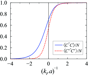
Figure 1: (Color online) The fraction of condensate particles $\langle C^{\dagger}C\rangle/N$ with two different definitions: (a) $\lambda_{k}\sim\tilde{u}_{k}\tilde{v}_{k}$ (solid line) (Eq.(14)) and (b)$\lambda_{k}^{\prime}\sim\tilde{v}_{k}/\tilde{u}_{k}$ (red dashed line) (Eq.(19)).

Using Eq. (23) for $\tilde{u}_{k}$ and $\tilde{v}_{k}$, we evaluate Eq. (14, 15) and Eq. (19, 20). In Fig. 1 we plot the fraction of condensation in the gas, as a function of the dimensionless parameter $(k_{F}a)^{-1}$. With either choice of $\lambda_{k}$, the fraction goes to one in the BEC limit $(k_{F}a)^{-1}\gg 1$. Notice that $\left\langle C^{\dagger}C\right\rangle/N$ is an appreciably higher fraction than $\left\langle C^{\prime{\dagger}}C^{\prime}\right\rangle/N$, showing a dominant condensation of atoms into the pair wave function defined in (12).

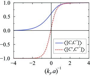
Figure 2: (Color online) Expectation value of the commutator $\langle\left[C,C^{\dagger}\right]\rangle$ with two different definitions: (a) $\lambda_{k}\sim\tilde{u}_{k}\tilde{v}_{k}$ (solid line) (Eq. (15)) and (b)$\lambda_{k}^{\prime}\sim\tilde{v}_{k}/\tilde{u}_{k}$ (red dashed line) Eq. (20)).

The expectation value of the commutator $\langle\left[C,C^{\dagger}\right]\rangle$ as a function of $(k_{F}a)^{-1}$ is shown in Fig. 2. Again both definitions of $\lambda_{k}$ give unity in the BEC limit, but Eq. (15) is always closer to one than Eq. (20).

Next we calculate the factor $\chi_{N+1}/\chi_{N}$. By solving Eq. (9) numerically for $\lambda_{k}$ and $\lambda_{k}^{\prime}$, we obtain the ratios $\chi_{N+1}/\chi_{N}$ and $\chi_{N+1}^{\prime}/\chi_{N}^{\prime}$ from Eq. (8). These ratios are shown in Fig. 3 as a function of $(k_{F}a)^{-1}$. We see that $\chi_{N+1}/\chi_{N}$ is closer to one throughout the transition region. Together with the tests based on expectation values above, $\lambda_{k}$ defined Eq. (13) seems to be a more suitable choice for the bosonic description of paired atoms.

Our calculations indicate an interesting region roughly at $-2\lesssim(k_{F}a)^{-1}\lesssim 2$ where Cooper pairs transit from being non-bosonic to bosonic. Note that it does not require $(k_{F}a)^{-1}\gg 1$ for the emergence of bosonic character. At $(k_{F}a)^{-1}=1$, the fraction of condensation $\langle C^{\dagger}C\rangle/N$ is already 95%, $\langle\left[C,C^{\dagger}\right]\rangle\sim 0.94$ and $\chi_{N+1}/\chi_{N}\sim 0.97$. In particular at the point where the chemical potential $\mu=0$ ($(k_{F}a)^{-1}\approx 0.553$) analytic , which is sometimes recognized as the boundary between BEC and BCS regimes Leggett2 ; Chen , we have $\langle\left[C,C^{\dagger}\right]\rangle=0.835$, $\chi_{N+1}/\chi_{N}=0.937$. The use of definition (18) gives slightly weaker numbers, but a narrower transition region.

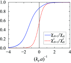
Figure 3: (Color online) The quantity $\chi_{N+1}/\chi_{N}$ with two different definitions: (a) $\lambda_{k}\sim\tilde{u}_{k}\tilde{v}_{k}$ (blue solid line) and (b)$\lambda_{k}^{\prime}\sim\tilde{v}_{k}/\tilde{u}_{k}$ (red dashed line).

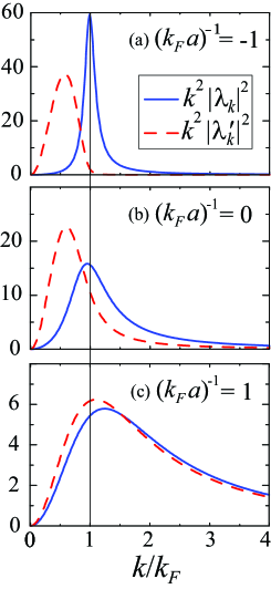
Figure 4: (Color online) Momentum distribution (in units of $k_{F}$) of two different Cooper pair wave functions, $\lambda_{k}\sim\tilde{u}_{k}\tilde{v}_{k}$ (blue line) and $\lambda_{k}^{\prime}\sim\tilde{v}_{k}/\tilde{u}_{k}$ (red dashed line). In (a) the BCS limit, two definitions differ significantly, while in (c) the BEC limit, two definitions overlap (see text).

V Conclusion

To conclude, three indicators were used to quantify the bosonic characters of a Cooper pair in an interacting Fermi gas : (a) $\langle C^{\dagger}C\rangle$, (b) $\langle\left[C,C^{\dagger}\right]\rangle$, (c) $\chi_{N+1}/\chi_{N}$. Two different definitions of a Cooper pair were examined, $\lambda_{n}^{\prime}\propto\tilde{v}_{n}/\tilde{u}_{n}$ and $\lambda_{n}\propto\tilde{u}^{*}_{n}\tilde{v}_{n}$. Our calculations suggest that the latter one provides a better description of the Cooper pairs as bosonic particles. Moreover, as the fraction of composite particles goes to one in the BEC limit, the gas is basically in its simplest single mode. It appears that using either one of the two definitions makes little differences in the strong coupling regime $(k_{F}a)^{-1}\geq 1$. This is consistent with the results in Ref. Ortiz , in which the authors addressed the similarity of both definitions. As shown in Fig. 4, the difference between (13) and (18) on the BCS side is that, the former only takes into account of a few momentum states on the Fermi surface, whereas the latter one takes the average of all states inside the Fermi sphere. In a weakly interacting gas, only atoms lying on the Fermi surface interact effectively, the composite particle based on (13) would thus be more bosonic since it takes into account the dominant correlated states. In the deep BEC limit, the Fermi sphere is totally smeared out, and either choice of $\lambda_{n}$ would weigh different momentum states on an almost equal footage, resulting in the merge of two different pictures.

If the system is not in the BEC limit, we have shown that the bosonic character of a Cooper pair depends on how the pair wave function is defined. Our work here is an attempt to identify what definition is more effective to reveal a Cooper pair as a boson. From an experimental point of view, it is interesting to search for observables associated with $C$ or $C^{\prime}$, so that one can probe the the quantum statistics of Cooper pairs directly. We also remark that our method can in principle be extended to nonuniform systems. However, the coefficients $\tilde{u}_{n}$ and $\tilde{v}_{n}$, which are calculated from the natural orbits German ; Pong , do not have closed forms for analytical discussions. The question how a trapping potential affects the bosonic properties of Cooper pairs is an open problem for future studies.

Appendix

We list here some integrals used in this paper. A detail analysis can be found in the paper by Marini et al. analytic and the paper by Ortiz et al. Ortiz . In the following list, we adopt the following change of variables,

$$x_{0}=\mu/\Delta,\;\;\;x^{2}=k^{2}/(2\Delta)$$ (26)

and introduce shorthand notations

$$\xi_{x} = x^{2}-x_{0},\;\;\;E_{x}=\sqrt{\xi_{x}^{2}+1},$$ (27)

$$\kappa^{2} = \frac{1}{2}\left(1+x_{0}/\sqrt{x_{0}^{2}+1}\right),$$ (28)

$$q = -x_{0}/\sqrt{x_{0}^{2}+1}.$$ (29)

So we have $\int k^{2}dk=\left(2\Delta\right)^{3/2}\int x^{2}dx$. Some integrals that appeared in our calculation are listed below

$$-\frac{1}{4\pi a} = \frac{\sqrt{2\Delta}}{2\pi^{2}}\int_{0}^{\infty}x^{2}dx\left(\frac{1}{E_{x}}-\frac{1}{x^{2}}\right)$$ (30)

$$\frac{N}{V} = \frac{\left(2\Delta\right)^{3/2}}{4\pi^{2}}\int_{0}^{\infty}x^{2}dx\left(1-\frac{\xi_{x}}{E_{x}}\right)$$ (31)

$$\int\frac{d^{3}k}{(2\pi)^{3}}\left|\tilde{u}_{k}\tilde{v}_{k}\right|^{2} = \frac{(2\Delta)^{3/2}}{8\pi^{2}}\int_{0}^{\infty}\frac{x^{2}dx}{E_{x}^{2}}$$ (32)

$$\int\frac{d^{3}k}{(2\pi)^{3}}\left|\frac{\tilde{v}_{k}}{\tilde{u}_{k}}\right|^{2} = \frac{(2\Delta)^{3/2}}{2\pi^{2}}\int_{0}^{\infty}x^{2}dx\frac{E_{x}-\xi_{x}}{E_{x}+\xi_{x}}$$ (33)

The integrals are expressed in terms of $K$ and $E$, which are respectively the complete elliptic integral of the first and second kind. We also need $P_{n}$, Legendre function of the first kind of degree $n$.

$$\int_{0}^{\infty}x^{2}dx\left(\frac{1}{E_{x}}-\frac{1}{x^{2}}\right)=\frac{K(\kappa^{2})-2E(\kappa^{2})}{\left(x_{0}^{2}+1\right)^{-1/4}}$$ (34)

$$\int_{0}^{\infty}\frac{x^{2}dx}{E_{x}^{2}}=\frac{\pi}{2\sqrt{2}}\sqrt{x_{0}+\sqrt{x_{0}^{2}+1}}.$$ (35)

$$\int_{0}^{\infty}x^{2}dx\left(1-\frac{\xi_{x}}{E_{x}}\right)=\frac{(1+q)K(\kappa^{2})-2qE(\kappa^{2})}{3(x_{0}^{2}+1)^{-3/4}}$$ (36)

$$\int_{0}^{\infty}x^{2}dx\frac{E_{x}-\xi_{x}}{E_{x}+\xi_{x}}$$

$$=\frac{2\pi}{35}\frac{\left(q^{2}-5\right)P_{3/2}\left(q\right)+4qP_{1/2}\left(q\right)}{(x_{0}^{2}+1)^{-7/4}}$$ (37)

Choosing $\lambda_{k}=\tilde{u}_{k}\tilde{v}_{k}/\sqrt{\sum_{\textbf{k}^{\prime}}|\tilde{u}_{k^{\prime}}\tilde{v}_{k^{\prime}}|^{2}}$, Eq. (9) is solved with the help of the following integral,

$$\int_{0}^{\infty}\frac{x^{2}dx}{bE_{x}^{2}+1} = \frac{\pi\sqrt{x_{0}+\sqrt{x_{0}^{2}+1+1/b}}}{\sqrt{8}\sqrt{b(b+1)}},$$ (38)

where $b$ is a positive real number. For $\lambda_{k}^{\prime}=(\tilde{v}_{k}/\tilde{u}_{k})/\sqrt{\sum_{\textbf{k}^{\prime}}|\tilde{v}_{k^{\prime}}/\tilde{u}_{k^{\prime}}|^{2}}$, Eq. (9) is numerically integrated and solved.

References

• (1) C. A. Regal, M. Greiner, and D. S. Jin, Phys. Rev. Lett. 92, 040403 (2004).
• (2) M. W. Zwierlein, C. A. Stan, C. H. Schunck, S. M. F. Raupach, A. J. Kerman, and W. Ketterle, Phys. Rev. Lett. 92, 120403 (2004); M. W. Zwierlein, J. R. Abo-Shaeer, A. Schirotzek, C. H. Schunck, and W. Ketterle, Nature 435, 1047 (2005).
• (3) Martin W. Zwierlein, Andre Schirotzek, Christian H. Schunck, and Wolfgang Ketterle, Science 311, 492 (2006).
• (4) M. Bartenstein, A. Altmeyer, S. Riedl, S. Jochim, C. Chin, J. Hecker Denschlag, R. Grimm, Phys. Rev. Lett. 92, 203201 (2004).
• (5) K. M. O’Hara, S. L. Hemmer, M. E. Gehm, S. R. Granade, J. E. Thomas, Science 298, 2179 (2002).
• (6) P. G. de Gennes, Superconductivity of Metals and Alloys (W.A. Benjamin INC.,1966); J. B. Ketterson and S. N. Song, Superconductivity (New York, Cambridge University Press, 1999).
• (7) P. NoziΓ©res, S. Schmitt-Rink, J. Low Temp. Phys. 59, 195 (1985).
• (8) M. Combescot and C. Tanguy, Europhys. Lett. 55, 390 (2001).
• (9) M. Combescot, X. Leyronas, and C. Tanguy, Eur. Phys. J. B 31, 17 (2003).
• (10) C. K. Law, Phys. Rev. A 71, 034306 (2005).
• (11) G. Ortiz and J. Dukelsky, Phys. Rev. A 72, 043611 (2005); G. Ortiz and J. Dukelsky, cond-mat/0604236.
• (12) C. N. Yang, Rev. Mod. Phys. 34, 694 (1962).
• (13) M. Randeria, in Bose Einstein Condensation, edited by A. Griffin, D. W. Snoke and S. Stringari (Cambridge University Press 1995).
• (14) Roberto B. Diener and Tin-Lun Ho, cond-mat/0404517.
• (15) Luca Salasnich, Nicola Manini, Alberto Parola, Phys. Rev. A 72, 023621 (2005).
• (16) M. Marini, F. Pistolesi, and G.C. Strinati, Eur. Phys. J. B 1, 151 (1998).
• (17) Meera M. Parish, Bogdan Mihaila, Eddy M. Timmermans, Krastan B. Blagoev, and Peter B. Littlewood, Phys. Rev. B 71, 064513 (2005).
• (18) P.-G. Reinhard, M. Bender, K. Rutz, and J. A. Maruhn, Z. Phys. A 358, 277 (1997).
• (19) Y.H. Pong and C. K. Law, Phys. Rev. A 74 013618 (2006).
• (20) A. J. Leggett, J. de Physique 41, C7-19 (1980).
• (21) A. J. Leggett, in Modern Trends in the Theory of Condensed Matter, edited by A. Pekalski and R. Przystawa (Springer-Verlag, Berlin, 1980).
• (22) Qijin Chen, Jelena Stajic, Shina Tan, and K. Levin, Phys. Rep. 412, 1 (2005).