Sparsity-certifying Graph Decompositions

Abstract

We describe a new algorithm, the $(k,\ell)$-pebble game with colors, and use it to obtain a characterization of the family of $(k,\ell)$-sparse graphs and algorithmic solutions to a family of problems concerning tree decompositions of graphs. Special instances of sparse graphs appear in rigidity theory and have received increased attention in recent years. In particular, our colored pebbles generalize and strengthen the previous results of Lee and Streinu [12] and give a new proof of the Tutte-Nash-Williams characterization of arboricity. We also present a new decomposition that certifies sparsity based on the $(k,\ell)$-pebble game with colors. Our work also exposes connections between pebble game algorithms and previous sparse graph algorithms by Gabow [5], Gabow and Westermann [6] and Hendrickson [9].

1 Introduction and preliminaries

The focus of this paper is decompositions of $(k,\ell)$-sparse graphs into edge-disjoint subgraphs that certify sparsity. We use graph to mean a multigraph, possibly with loops. We say that a graph is $(k,\ell)$-sparse if no subset of $n^{\prime}$ vertices spans more than $kn^{\prime}-\ell$ edges in the graph; a $(k,\ell)$-sparse graph with $kn^{\prime}-\ell$ edges is $(k,\ell)$-tight. We call the range $k\leq\ell\leq 2k-1$ the upper range of sparse graphs and $0\leq\ell\leq k$ the lower range.

In this paper, we present efficient algorithms for finding decompositions that certify sparsity in the upper range of $\ell$. Our algorithms also apply in the lower range, which was already addressed by [5, 6, 3, 19, 4]. A decomposition certifies the sparsity of a graph if the sparse graphs and graphs admitting the decomposition coincide.

Our algorithms are based on a new characterization of sparse graphs, which we call the pebble game with colors. The pebble game with colors is a simple graph construction rule that produces a sparse graph along with a sparsity-certifying decomposition.

We define and study a canonical class of pebble game constructions, which correspond to previously studied decompositions of sparse graphs into edge disjoint trees. Our results provide a unifying framework for all the previously known special cases, including Nash-Williams-Tutte and [24, 7]. Indeed, in the lower range, canonical pebble game constructions capture the properties of the augmenting paths used in matroid union and intersection algorithms[5, 6]. Since the sparse graphs in the upper range are not known to be unions or intersections of the matroids for which there are efficient augmenting path algorithms, these do not easily apply in the upper range. Pebble game with colors constructions may thus be considered a strengthening of augmenting paths to the upper range of matroidal sparse graphs.

1.1 Sparse graphs

A graph is $(k,\ell)$-sparse if for any non-empty subgraph with $m^{\prime}$ edges and $n^{\prime}$ vertices, $m^{\prime}\leq kn^{\prime}-\ell.$ We observe that this condition implies that $0\leq\ell\leq 2k-1$, and from now on in this paper we will make this assumption. A sparse graph that has $n$ vertices and exactly $kn-\ell$ edges is called tight.

For a graph $G=(V,E)$, and $V^{\prime}\subset V$, we use the notation $\operatorname{span}(V^{\prime})$ for the number of edges in the subgraph induced by $V^{\prime}$. In a directed graph, $\operatorname{out}(V^{\prime})$ is the number of edges with the tail in $V^{\prime}$ and the head in $V-V^{\prime}$; for a subgraph induced by $V^{\prime}$, we call such an edge an out-edge.

There are two important types of subgraphs of sparse graphs. A block is a tight subgraph of a sparse graph. A component is a maximal block.

Term	Meaning
Sparse graph $G$	Every non-empty subgraph on $n^{\prime}$ vertices has $\leq kn^{\prime}-\ell$ edges
Tight graph $G$	$G=(V,E)$ is sparse and $\left|V\right|=n$, $\left|E\right|=kn-\ell$
Block $H$ in $G$	$G$ is sparse, and $H$ is a tight subgraph
Component $H$ of $G$	$G$ is sparse and $H$ is a maximal block
Map-graph	Graph that admits an out-degree-exactly-one orientation
$(k,\ell)$-maps-and-trees	Edge-disjoint union of $\ell$ trees and $(k-\ell)$ map-grpahs
$\ell{\mathsf{T}}k$	Union of $\ell$ trees, each vertex is in exactly $k$ of them
Set of tree-pieces of an $\ell{\mathsf{T}}k\,$ induced on $V^{\prime}\subset V$	Pieces of trees in the $\ell{\mathsf{T}}k$ spanned by $E(V^{\prime})$
Proper $\ell{\mathsf{T}}k$	Every $V^{\prime}\subset V$ contains $\geq\ell$ pieces of trees from the $\ell{\mathsf{T}}k$

Table 1: Sparse graph and decomposition terminology used in this paper.

Table 1 summarizes the sparse graph terminology used in this paper.

1.2 Sparsity-certifying decompositions

A $k$-arborescence is a graph that admits a decomposition into $k$ edge-disjoint spanning trees. Figure 1 shows an example of a $3$-arborescence. The $k$-arborescent graphs are described by the well-known theorems of Tutte [23] and Nash-Williams [17] as exactly the $(k,k)$-tight graphs.

A map-graph is a graph that admits an orientation such that the out-degree of each vertex is exactly one. A $k$-map-graph is a graph that admits a decomposition into $k$ edge-disjoint map-graphs. Figure 1 shows an example of a 2-map-graphs; the edges are oriented in one possible configuration certifying that each color forms a map-graph. Map-graphs may be equivalently defined (see, e.g., [18]) as having exactly one cycle per connected component.

A $(k,\ell)$-maps-and-trees is a graph that admits a decomposition into $k-\ell$ edge-disjoint map-graphs and $\ell$ spanning trees.

Another characterization of map-graphs, which we will use extensively in this paper, is as the $(1,0)$-tight graphs [24, 8]. The $k$-map-graphs are evidently $(k,0)$-tight, and [24, 8] show that the converse holds as well.

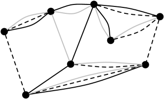
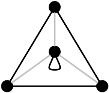
Figure 1: Examples of sparsity-certifying decompositions: (a) a $3$-arborescence; (b) a 2-map-graph; (c) a $(2,1)$-maps-and-trees. Edges with the same line style belong to the same subgraph. The 2-map-graph is shown with a certifying orientation.

A $\ell{\mathsf{T}}k$ is a decomposition into $\ell$ edge-disjoint (not necessarily spanning) trees such that each vertex is in exactly $k$ of them. Figure 2 shows an example of a $3{\mathsf{T}}2$.

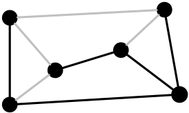
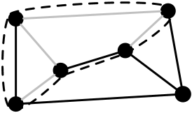
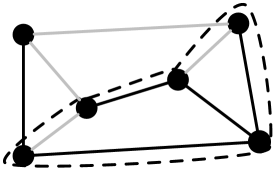
Figure 2: (a) A graph with a $3\mathsf{T}2$ decomposition; one of the three trees is a single vertex in the bottom right corner. (b) The highlighted subgraph inside the dashed countour has three black tree-pieces and one gray tree-piece. (c) The highlighted subgraph inside the dashed countour has three gray tree-pieces (one is a single vertex) and one black tree-piece.

Given a subgraph $G^{\prime}$ of a $\ell{\mathsf{T}}k$ graph $G$, the set of tree-pieces in $G^{\prime}$ is the collection of the components of the trees in $G$ induced by $G^{\prime}$ (since $G^{\prime}$ is a subgraph each tree may contribute multiple pieces to the set of tree-pieces in $G^{\prime}$). We observe that these tree-pieces may come from the same tree or be single-vertex “empty trees.” It is also helpful to note that the definition of a tree-piece is relative to a specific subgraph. An $\ell{\mathsf{T}}k$ decomposition is proper if the set of tree-pieces in any subgraph $G^{\prime}$ has size at least $\ell$.

Figure 2 shows a graph with a $3\mathsf{T}2$ decomposition; we note that one of the trees is an isolated vertex in the bottom-right corner. The subgraph in Figure 2 has three black tree-pieces and one gray tree-piece: an isolated vertex at the top-right corner, and two single edges. These count as three tree-pieces, even though they come from the same back tree when the whole graph in considered. Figure 2 shows another subgraph; in this case there are three gray tree-pieces and one black one.

Table 1 contains the decomposition terminology used in this paper.

The decomposition problem.

We define the decomposition problem for sparse graphs as taking a graph as its input and producing as output, a decomposition that can be used to certify sparsity. In this paper, we will study three kinds of outputs: maps-and-trees; proper $\ell{\mathsf{T}}k$ decompositions; and the pebble-game-with-colors decomposition, which is defined in the next section.

2 Historical background

The well-known theorems of Tutte [23] and Nash-Williams [17] relate the $(k,k)$-tight graphs to the existence of decompositions into edge-disjoint spanning trees. Taking a matroidal viewpoint, Edmonds [3, 4] gave another proof of this result using matroid unions. The equivalence of maps-and-trees graphs and tight graphs in the lower range is shown using matroid unions in [24], and matroid augmenting paths are the basis of the algorithms for the lower range of [19, 5, 6].

In rigidity theory a foundational theorem of Laman [11] shows that $(2,3)$-tight (Laman) graphs correspond to generically minimally rigid bar-and-joint frameworks in the plane. Tay [21] proved an analogous result for body-bar frameworks in any dimension using $(k,k)$-tight graphs. Rigidity by counts motivated interest in the upper range, and Crapo [2] proved the equivalence of Laman graphs and proper $3\mathsf{T}2$ graphs. Tay [22] used this condition to give a direct proof of Laman’s theorem and generalized the $3\mathsf{T}2$ condition to all $\ell\mathsf{T}k$ for $k\leq\ell\leq 2k-1$. Haas [7] studied $\ell{\mathsf{T}}k$ decompositions in detail and proved the equivalence of tight graphs and proper $\ell{\mathsf{T}}k$ graphs for the general upper range. We observe that aside from our new pebble-game-with-colors decomposition, all the combinatorial characterizations of the upper range of sparse graphs, including the counts, have a geometric interpretation [24, 11, 22, 21].

A pebble game algorithm was first proposed in [10] as an elegant alternative to Hendrickson’s Laman graph algorithms [9]. Berg and Jordan [1], provided the formal analysis of the pebble game of [10] and introduced the idea of playing the game on a directed graph. Lee and Streinu [12] generalized the pebble game to the entire range of parameters $0\leq\ell\leq 2k-1$, and left as an open problem using the pebble game to find sparsity certifying decompositions.

3 The pebble game with colors

Our pebble game with colors is a set of rules for constructing graphs indexed by nonnegative integers $k$ and $\ell$. We will use the pebble game with colors as the basis of an efficient algorithm for the decomposition problem later in this paper. Since the phrase “with colors” is necessary only for comparison to [12], we will omit it in the rest of the paper when the context is clear.

We now present the pebble game with colors. The game is played by a single player on a fixed finite set of vertices. The player makes a finite sequence of moves; a move consists in the addition and/or orientation of an edge. At any moment of time, the state of the game is captured by a directed graph $H$, with colored pebbles on vertices and edges. The edges of $H$ are colored by the pebbles on them. While playing the pebble game all edges are directed, and we use the notation $vw$ to indicate a directed edge from $v$ to $w$.

We describe the pebble game with colors in terms of its initial configuration and the allowed moves.

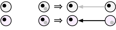
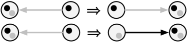
Figure 3: Examples of pebble game with colors moves: (a) add-edge. (b) pebble-slide. Pebbles on vertices are shown as black or gray dots. Edges are colored with the color of the pebble on them.

Initialization: In the beginning of the pebble game, $H$ has $n$ vertices and no edges. We start by placing $k$ pebbles on each vertex of $H$, one of each color $c_{i}$, for $i=1,2,\ldots,k$.

Add-edge-with-colors: Let $v$ and $w$ be vertices with at least $\ell+1$ pebbles on them. Assume (w.l.o.g.) that $v$ has at least one pebble on it. Pick up a pebble from $v$, add the oriented edge $vw$ to $E(H)$ and put the pebble picked up from $v$ on the new edge.

Figure 3 shows examples of the add-edge move.

Pebble-slide: Let $w$ be a vertex with a pebble $p$ on it, and let $vw$ be an edge in $H$. Replace $vw$ with $wv$ in $E(H)$; put the pebble that was on $vw$ on $v$; and put $p$ on $wv$.

Note that the color of an edge can change with a pebble-slide move. Figure 3 shows examples. The convention in these figures, and throughout this paper, is that pebbles on vertices are represented as colored dots, and that edges are shown in the color of the pebble on them.

From the definition of the pebble-slide move, it is easy to see that a particular pebble is always either on the vertex where it started or on an edge that has this vertex as the tail. However, when making a sequence of pebble-slide moves that reverse the orientation of a path in $H$, it is sometimes convenient to think of this path reversal sequence as bringing a pebble from the end of the path to the beginning.

The output of playing the pebble game is its complete configuration.

Output: At the end of the game, we obtain the directed graph $H$, along with the location and colors of the pebbles. Observe that since each edge has exactly one pebble on it, the pebble game configuration colors the edges.

We say that the underlying undirected graph $G$ of $H$ is constructed by the $(k,\ell)$-pebble game or that $H$ is a pebble-game graph.

Since each edge of $H$ has exactly one pebble on it, the pebble game’s configuration partitions the edges of $H$, and thus $G$, into $k$ different colors. We call this decomposition of $H$ a pebble-game-with-colors decomposition. Figure 4 shows an example of a $(2,2)$-tight graph with a pebble-game decomposition.

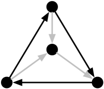
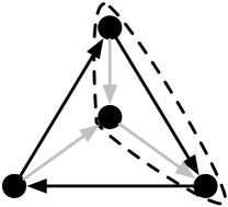
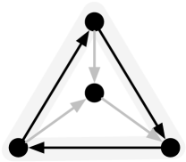
Figure 4: A $(2,2)$-tight graph with one possible pebble-game decomposition. The edges are oriented to show $(1,0)$-sparsity for each color. (a) The graph $K_{4}$ with a pebble-game decomposition. There is an empty black tree at the center vertex and a gray spanning tree. (b) The highlighted subgraph has two black trees and a gray tree; the black edges are part of a larger cycle but contribute a tree to the subgraph. (c) The highlighted subgraph (with a light gray background) has three empty gray trees; the black edges contain a cycle and do not contribute a piece of tree to the subgraph.

Let $G=(V,E)$ be pebble-game graph with the coloring induced by the pebbles on the edges, and let $G^{\prime}$ be a subgraph of $G$. Then the coloring of $G$ induces a set of monochromatic connected subgraphs of $G^{\prime}$ (there may be more than one of the same color). Such a monochromatic subgraph is called a map-graph-piece of $G^{\prime}$ if it contains a cycle (in $G^{\prime}$) and a tree-piece of $G^{\prime}$ otherwise. The set of tree-pieces of $G^{\prime}$ is the collection of tree-pieces induced by $G^{\prime}$. As with the corresponding definition for $\ell{\mathsf{T}}k\,$s, the set of tree-pieces is defined relative to a specific subgraph; in particular a tree-piece may be part of a larger cycle that includes edges not spanned by $G^{\prime}$.

The properties of pebble-game decompositions are studied in Section 6, and Theorem 2 shows that each color must be $(1,0)$-sparse. The orientation of the edges in Figure 4 shows this.

For example Figure 4 shows a $(2,2)$-tight graph with one possible pebble-game decomposition. The whole graph contains a gray tree-piece and a black tree-piece that is an isolated vertex. The subgraph in Figure 4 has a black tree and a gray tree, with the edges of the black tree coming from a cycle in the larger graph. In Figure 4, however, the black cycle does not contribute a tree-piece. All three tree-pieces in this subgraph are single-vertex gray trees.

In the following discussion, we use the notation $\operatorname{peb}(v)$ for the number of pebbles on $v$ and $\operatorname{peb}_{i}(v)$ to indicate the number of pebbles of colors $i$ on $v$.

Table 2 lists the pebble game notation used in this paper.

Notation	Meaning
$\operatorname{span}(V^{\prime})$	Number of edges spanned in $H$ by $V^{\prime}\subset V$; i.e. $\left|E_{H}(V^{\prime})\right|$
$\operatorname{peb}(V^{\prime})$	Number of pebbles on $V^{\prime}\subset V$
$\operatorname{out}(V^{\prime})$	Number of edges $vw$ in $H$ with $v\in V^{\prime}$ and $w\in V-V^{\prime}$
$\operatorname{peb}_{i}(v)$	Number of pebbles of color $c_{i}$ on $v\in V$
$\operatorname{out}_{i}(v)$	Number of edges $vw$ colored $c_{i}$ for $v\in V$

Table 2: Pebble game notation used in this paper.

4 Our Results

We describe our results in this section. The rest of the paper provides the proofs.

Our first result is a strengthening of the pebble games of [12] to include colors. It says that sparse graphs are exactly pebble game graphs. Recall that from now on, all pebble games discussed in this paper are our pebble game with colors unless noted explicitly.

Theorem 1 (Sparse graphs and pebble-game graphs coincide).

A graph $G$ is $(k,\ell)$-sparse with $0\leq\ell\leq 2k-1$ if and only if $G$ is a pebble-game graph.

Next we consider pebble-game decompositions, showing that they are a generalization of proper $\ell{\mathsf{T}}k$ decompositions that extend to the entire matroidal range of sparse graphs.

Theorem 2 (The pebble-game-with-colors decomposition).

A graph $G$ is a pebble-game graph if and only if it admits a decomposition into $k$ edge-disjoint subgraphs such that each is $(1,0)$-sparse and every subgraph of $G$ contains at least $\ell$ tree-pieces of the $(1,0)$-sparse graphs in the decomposition.

The $(1,0)$-sparse subgraphs in the statement of Theorem 2 are the colors of the pebbles; thus Theorem 2 gives a characterization of the pebble-game-with-colors decompositions obtained by playing the pebble game defined in the previous section. Notice the similarity between the requirement that the set of tree-pieces have size at least $\ell$ in Theorem 2 and the definition of a proper $\ell{\mathsf{T}}k\,$.

Our next results show that for any pebble-game graph, we can specialize its pebble game construction to generate a decomposition that is a maps-and-trees or proper $\ell{\mathsf{T}}k$ . We call these specialized pebble game constructions canonical, and using canonical pebble game constructions, we obtain new direct proofs of existing arboricity results.

We observe Theorem 2 that maps-and-trees are special cases of the pebble-game decomposition: both spanning trees and spanning map-graphs are $(1,0)$-sparse, and each of the spanning trees contributes at least one piece of tree to every subgraph.

The case of proper $\ell{\mathsf{T}}k$ graphs is more subtle; if each color in a pebble-game decomposition is a forest, then we have found a proper $\ell{\mathsf{T}}k$ , but this class is a subset of all possible proper $\ell{\mathsf{T}}k$ decompositions of a tight graph. We show that this class of proper $\ell{\mathsf{T}}k$ decompositions is sufficient to certify sparsity.

We now state the main theorem for the upper and lower range.

Theorem 3 (Main Theorem (Lower Range): Maps-and-trees coincide with pebble-game graphs).

Let $0\leq\ell\leq k$. A graph $G$ is a tight pebble-game graph if and only if $G$ is a $(k,\ell)$-maps-and-trees.

Theorem 4 (Main Theorem (Upper Range): Proper $\ell{\mathsf{T}}k$ graphs coincide with pebble-game graphs).

Let $k\leq\ell\leq 2k-1$. A graph $G$ is a tight pebble-game graph if and only if it is a proper $\ell{\mathsf{T}}k$ with $kn-\ell$ edges.

As corollaries, we obtain the existing decomposition results for sparse graphs.

Corollary 5 (Nash-Williams [17], Tutte [23], White and Whiteley [24]).

Let $\ell\leq k$. A graph $G$ is tight if and only if has a $(k,\ell)$-maps-and-trees decomposition.

Corollary 6 (Crapo [2], Haas [7]).

Let $k\leq\ell\leq 2k-1$. A graph $G$ is tight if and only if it is a proper $\ell{\mathsf{T}}k$ .

Efficiently finding canonical pebble game constructions.

The proofs of Theorem 3 and Theorem 4 lead to an obvious algorithm with $O(n^{3})$ running time for the decomposition problem. Our last result improves on this, showing that a canonical pebble game construction, and thus a maps-and-trees or proper $\ell{\mathsf{T}}k$ decomposition can be found using a pebble game algorithm in $O(n^{2})$ time and space.

These time and space bounds mean that our algorithm can be combined with those of [12] without any change in complexity.

5 Pebble game graphs

In this section we prove Theorem 1, a strengthening of results from [12] to the pebble game with colors. Since many of the relevant properties of the pebble game with colors carry over directly from the pebble games of [12], we refer the reader there for the proofs.

We begin by establishing some invariants that hold during the execution of the pebble game.

Lemma 7 (Pebble game invariants).

During the execution of the pebble game, the following invariants are maintained in $H$:

1. There are at least $\ell$ pebbles on $V$. [12]

2. For each vertex $v$, $\operatorname{span}(v)+\operatorname{out}(v)+\operatorname{peb}(v)=k$. [12]

3. For each $V^{\prime}\subset V$, $\operatorname{span}(V^{\prime})+\operatorname{out}(V^{\prime})+\operatorname{peb}(V^{\prime})=kn^{\prime}$. [12]

4. For every vertex $v\in V$, $\operatorname{out}_{i}(v)+\operatorname{peb}_{i}(v)=1$.

5. Every maximal path consisting only of edges with color $c_{i}$ ends in either the first vertex with a pebble of color $c_{i}$ or a cycle.

Proof.

(I1), (I2), and (I3) come directly from [12].

(I4) This invariant clearly holds at the initialization phase of the pebble game with colors. That add-edge and pebble-slide moves preserve (I4) is clear from inspection.

(I5) By (I4), a monochromatic path of edges is forced to end only at a vertex with a pebble of the same color on it. If there is no pebble of that color reachable, then the path must eventually visit some vertex twice. ∎

From these invariants, we can show that the pebble game constructible graphs are sparse.

Lemma 8 (Pebble-game graphs are sparse [12]).

Let $H$ be a graph constructed with the pebble game. Then $H$ is sparse. If there are exactly $\ell$ pebbles on $V(H)$, then $H$ is tight.

The main step in proving that every sparse graph is a pebble-game graph is the following. Recall that by bringing a pebble to $v$ we mean reorienting $H$ with pebble-slide moves to reduce the out degree of $v$ by one.

Lemma 9 (The $\ell+1$ pebble condition [12]).

Let $vw$ be an edge such that $H+vw$ is sparse. If $\operatorname{peb}(\{v,w\})<\ell+1$, then a pebble not on $\{v,w\}$ can be brought to either $v$ or $w$.

It follows that any sparse graph has a pebble game construction. [Sparse graphs and pebble-game graphs coincide] A graph $G$ is $(k,\ell)$-sparse with $0\leq\ell\leq 2k-1$ if and only if $G$ is a pebble-game graph.

6 The pebble-game-with-colors decomposition

In this section we prove Theorem 2, which characterizes all pebble-game decompositions. We start with the following lemmas about the structure of monochromatic connected components in $H$, the directed graph maintained during the pebble game.

Lemma 10 (Monochromatic pebble game subgraphs are $(1,0)$-sparse).

Let $H_{i}$ be the subgraph of $H$ induced by edges with pebbles of color $c_{i}$ on them. Then $H_{i}$ is $(1,0)$-sparse, for $i=1,\ldots,k$.

Proof.

By (I4) $H_{i}$ is a set of edges with out degree at most one for every vertex.

∎

Lemma 11 (Tree-pieces in a pebble-game graph).

Every subgraph of the directed graph $H$ in a pebble game construction contains at least $\ell$ monochromatic tree-pieces, and each of these is rooted at either a vertex with a pebble on it or a vertex that is the tail of an out-edge.

Recall that an out-edge from a subgraph $H^{\prime}=(V^{\prime},E^{\prime})$ is an edge $vw$ with $v\in V^{\prime}$ and $vw\notin E^{\prime}$.

Proof.

Let $H^{\prime}=(V^{\prime},E^{\prime})$ be a non-empty subgraph of $H$, and assume without loss of generality that $H^{\prime}$ is induced by $V^{\prime}$. By (I3), $\operatorname{out}(V^{\prime})+\operatorname{peb}(V^{\prime})\geq\ell$. We will show that each pebble and out-edge tail is the root of a tree-piece.

Consider a vertex $v\in V^{\prime}$ and a color $c_{i}$. By (I4) there is a unique monochromatic directed path of color $c_{i}$ starting at $v$. By (I5), if this path ends at a pebble, it does not have a cycle. Similarly, if this path reaches a vertex that is the tail of an out-edge also in color $c_{i}$ (i.e., if the monochromatic path from $v$ leaves $V^{\prime}$), then the path cannot have a cycle in $H^{\prime}$.

Since this argument works for any vertex in any color, for each color there is a partitioning of the vertices into those that can reach each pebble, out-edge tail, or cycle. It follows that each pebble and out-edge tail is the root of a monochromatic tree, as desired. ∎

Applied to the whole graph Lemma 11 gives us the following.

Lemma 12 (Pebbles are the roots of trees).

In any pebble game configuration, each pebble of color $c_{i}$ is the root of a (possibly empty) monochromatic tree-piece of color $c_{i}$.

Remark: Haas showed in [7] that in a $\ell{\mathsf{T}}k$ , a subgraph induced by $n^{\prime}\geq 2$ vertices with $m^{\prime}$ edges has exactly $kn^{\prime}-m^{\prime}$ tree-pieces in it. Lemma 11 strengthens Haas’ result by extending it to the lower range and giving a construction that finds the tree-pieces, showing the connection between the $\ell+1$ pebble condition and the hereditary condition on proper $\ell{\mathsf{T}}k$ .

We conclude our investigation of arbitrary pebble game constructions with a description of the decomposition induced by the pebble game with colors.

[The pebble-game-with-colors decomposition] A graph $G$ is a pebble-game graph if and only if it admits a decomposition into $k$ edge-disjoint subgraphs such that each is $(1,0)$-sparse and every subgraph of $G$ contains at least $\ell$ tree-pieces of the $(1,0)$-sparse graphs in the decomposition.

Proof.

Let $G$ be a pebble-game graph. The existence of the $k$ edge-disjoint $(1,0)$-sparse subgraphs was shown in Lemma 10, and Lemma 11 proves the condition on subgraphs.

For the other direction, we observe that a color $c_{i}$ with $t_{i}$ tree-pieces in a given subgraph can span at most $n-t_{i}$ edges; summing over all the colors shows that a graph with a pebble-game decomposition must be sparse. Apply Theorem 1 to complete the proof. ∎

Remark: We observe that a pebble-game decomposition for a Laman graph may be read out of the bipartite matching used in Hendrickson’s Laman graph extraction algorithm [9]. Indeed, pebble game orientations have a natural correspondence with the bipartite matchings used in [9].

Maps-and-trees are a special case of pebble-game decompositions for tight graphs: if there are no cycles in $\ell$ of the colors, then the trees rooted at the corresponding $\ell$ pebbles must be spanning, since they have $n-1$ edges. Also, if each color forms a forest in an upper range pebble-game decomposition, then the tree-pieces condition ensures that the pebble-game decomposition is a proper $\ell{\mathsf{T}}k\,$.

In the next section, we show that the pebble game can be specialized to correspond to maps-and-trees and proper $\ell{\mathsf{T}}k$ decompositions.

7 Canonical Pebble Game Constructions

In this section we prove the main theorems (Theorem 3 and Theorem 4), continuing the investigation of decompositions induced by pebble game constructions by studying the case where a minimum number of monochromatic cycles are created. The main idea, captured in Lemma 15 and illustrated in Figure 6, is to avoid creating cycles while collecting pebbles. We show that this is always possible, implying that monochromatic map-graphs are created only when we add more than $k(n^{\prime}-1)$ edges to some set of $n^{\prime}$ vertices. For the lower range, this implies that every color is a forest. Every decomposition characterization of tight graphs discussed above follows immediately from the main theorem, giving new proofs of the previous results in a unified framework.

In the proof, we will use two specializations of the pebble game moves. The first is a modification of the add-edge move.

Canonical add-edge: When performing an add-edge move, cover the new edge with a color that is on both vertices if possible. If not, then take the highest numbered color present.

The second is a restriction on which pebble-slide moves we allow.

Canonical pebble-slide: A pebble-slide move is allowed only when it does not create a monochromatic cycle.

We call a pebble game construction that uses only these moves canonical. In this section we will show that every pebble-game graph has a canonical pebble game construction (Lemma 14 and Lemma 15) and that canonical pebble game constructions correspond to proper $\ell{\mathsf{T}}k$ and maps-and-trees decompositions (Theorem 3 and Theorem 4).

We begin with a technical lemma that motivates the definition of canonical pebble game constructions. It shows that the situations disallowed by the canonical moves are all the ways for cycles to form in the lowest $\ell$ colors.

Lemma 13 (Monochromatic cycle creation).

Let $v\in V$ have a pebble $p$ of color $c_{i}$ on it and let $w$ be a vertex in the same tree of color $c_{i}$ as $v$. A monochromatic cycle colored $c_{i}$ is created in exactly one of the following ways:

1. The edge $vw$ is added with an add-edge move.

2. The edge $wv$ is reversed by a pebble-slide move and the pebble $p$ is used to cover the reverse edge $vw$.

Proof.

Observe that the preconditions in the statement of the lemma are implied by Lemma 7. By Lemma 12 monochromatic cycles form when the last pebble of color $c_{i}$ is removed from a connected monochromatic subgraph. (M1) and (M2) are the only ways to do this in a pebble game construction, since the color of an edge only changes when it is inserted the first time or a new pebble is put on it by a pebble-slide move. ∎

Figure 5 and Figure 5 show examples of (M1) and (M2) map-graph creation moves, respectively, in a $(2,0)$-pebble game construction.

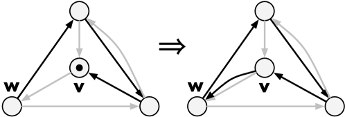
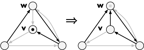
Figure 5: Creating monochromatic cycles in a $(2,0)$-pebble game. (a) A type (M1) move creates a cycle by adding a black edge. (b) A type (M2) move creates a cycle with a pebble-slide move. The vertices are labeled according to their role in the definition of the moves.

We next show that if a graph has a pebble game construction, then it has a canonical pebble game construction. This is done in two steps, considering the cases (M1) and (M2) separately. The proof gives two constructions that implement the canonical add-edge and canonical pebble-slide moves.

Lemma 14 (The canonical add-edge move).

Let $G$ be a graph with a pebble game construction. Cycle creation steps of type (M1) can be eliminated in colors $c_{i}$ for $1\leq i\leq\ell^{\prime}$, where $\ell^{\prime}=\min\{k,\ell\}$.

Proof.

For add-edge moves, cover the edge with a color present on both $v$ and $w$ if possible. If this is not possible, then there are $\ell+1$ distinct colors present. Use the highest numbered color to cover the new edge. ∎

Remark: We note that in the upper range, there is always a repeated color, so no canonical add-edge moves create cycles in the upper range.

The canonical pebble-slide move is defined by a global condition. To prove that we obtain the same class of graphs using only canonical pebble-slide moves, we need to extend Lemma 9 to only canonical moves. The main step is to show that if there is any sequence of moves that reorients a path from $v$ to $w$, then there is a sequence of canonical moves that does the same thing.

Lemma 15 (The canonical pebble-slide move).

Any sequence of pebble-slide moves leading to an add-edge move can be replaced with one that has no (M2) steps and allows the same add-edge move.

In other words, if it is possible to collect $\ell+1$ pebbles on the ends of an edge to be added, then it is possible to do this without creating any monochromatic cycles.

Figure 7 and Figure 8 illustrate the construction used in the proof of Lemma 15. We call this the shortcut construction by analogy to matroid union and intersection augmenting paths used in previous work on the lower range.

Figure 6 shows the structure of the proof. The shortcut construction removes an (M2) step at the beginning of a sequence that reorients a path from $v$ to $w$ with pebble-slides. Since one application of the shortcut construction reorients a simple path from a vertex $w^{\prime}$ to $w$, and a path from $v$ to $w^{\prime}$ is preserved, the shortcut construction can be applied inductively to find the sequence of moves we want.

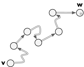
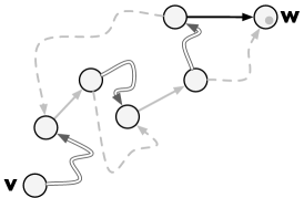
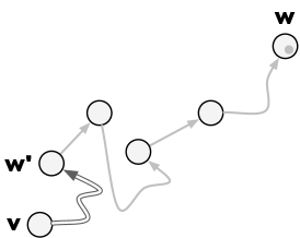
Figure 6: Outline of the shortcut construction: (a) An arbitrary simple path from $v$ to $w$ with curved lines indicating simple paths. (b) An (M2) step. The black edge, about to be flipped, would create a cycle, shown in dashed and solid gray, of the (unique) gray tree rooted at $w$. The solid gray edges were part of the original path from (a). (c) The shortened path to the gray pebble; the new path follows the gray tree all the way from the first time the original path touched the gray tree at $w^{\prime}$. The path from $v$ to $w^{\prime}$ is simple, and the shortcut construction can be applied inductively to it.

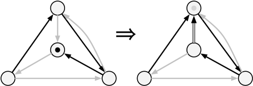
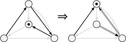
Figure 7: Eliminating (M2) moves: (a) an (M2) move; (b) avoiding the (M2) by moving along another path. The path where the pebbles move is indicated by doubled lines.

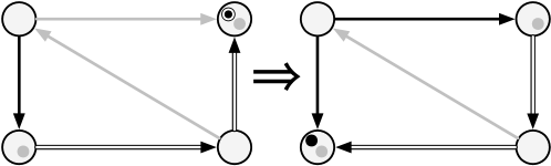
Figure 8: Eliminating (M2) moves: (a) the first step to move the black pebble along the doubled path is (M2); (b) avoiding the (M2) and simplifying the path.

Proof.

Without loss of generality, we can assume that our sequence of moves reorients a simple path in $H$, and that the first move (the end of the path) is (M2). The (M2) step moves a pebble of color $c_{i}$ from a vertex $w$ onto the edge $vw$, which is reversed. Because the move is (M2), $v$ and $w$ are contained in a maximal monochromatic tree of color $c_{i}$. Call this tree $H^{\prime}_{i}$, and observe that it is rooted at $w$.

Now consider the edges reversed in our sequence of moves. As noted above, before we make any of the moves, these sketch out a simple path in $H$ ending at $w$. Let $z$ be the first vertex on this path in $H^{\prime}_{i}$. We modify our sequence of moves as follows: delete, from the beginning, every move before the one that reverses some edge $yz$; prepend onto what is left a sequence of moves that moves the pebble on $w$ to $z$ in $H^{\prime}_{i}$.

Since no edges change color in the beginning of the new sequence, we have eliminated the (M2) move. Because our construction does not change any of the edges involved in the remaining tail of the original sequence, the part of the original path that is left in the new sequence will still be a simple path in $H$, meeting our initial hypothesis.

The rest of the lemma follows by induction. ∎

Together Lemma 14 and Lemma 15 prove the following.

Lemma 16.

If $G$ is a pebble-game graph, then $G$ has a canonical pebble game construction.

Using canonical pebble game constructions, we can identify the tight pebble-game graphs with maps-and-trees and $\ell{\mathsf{T}}k$   graphs.

[Main Theorem (Lower Range): Maps-and-trees coincide with pebble-game graphs] Let $0\leq\ell\leq k$. A graph $G$ is a tight pebble-game graph if and only if $G$ is a $(k,\ell)$-maps-and-trees.

Proof.

As observed above, a maps-and-trees decomposition is a special case of the pebble game decomposition. Applying Theorem 2, we see that any maps-and-trees must be a pebble-game graph.

For the reverse direction, consider a canonical pebble game construction of a tight graph. From Lemma 8, we see that there are $\ell$ pebbles left on $G$ at the end of the construction. The definition of the canonical add-edge move implies that there must be at least one pebble of each $c_{i}$ for $i=1,2,\ldots,\ell$. It follows that there is exactly one of each of these colors. By Lemma 12, each of these pebbles is the root of a monochromatic tree-piece with $n-1$ edges, yielding the required $\ell$ edge-disjoint spanning trees. ∎

[Nash-Williams [17], Tutte [23], White and Whiteley [24]] Let $\ell\leq k$. A graph $G$ is tight if and only if has a $(k,\ell)$-maps-and-trees decomposition.

We next consider the decompositions induced by canonical pebble game constructions when $\ell\geq k+1$. [Main Theorem (Upper Range): Proper Trees-and-trees coincide with pebble-game graphs] Let $k\leq\ell\leq 2k-1$. A graph $G$ is a tight pebble-game graph if and only if it is a proper $\ell{\mathsf{T}}k$ with $kn-\ell$ edges.

Proof.

As observed above, a proper $\ell{\mathsf{T}}k$ decomposition must be sparse. What we need to show is that a canonical pebble game construction of a tight graph produces a proper $\ell{\mathsf{T}}k$ .

By Theorem 2 and Lemma 16, we already have the condition on tree-pieces and the decomposition into $\ell$ edge-disjoint trees. Finally, an application of (I4), shows that every vertex must in in exactly $k$ of the trees, as required. ∎

[Crapo [2], Haas [7]] Let $k\leq\ell\leq 2k-1$. A graph $G$ is tight if and only if it is a proper $\ell{\mathsf{T}}k$ .

8 Pebble game algorithms for finding decompositions

A naïve implementation of the constructions in the previous section leads to an algorithm requiring $\Theta(n^{2})$ time to collect each pebble in a canonical construction: in the worst case $\Theta(n)$ applications of the construction in Lemma 15 requiring $\Theta(n)$ time each, giving a total running time of $\Theta(n^{3})$ for the decomposition problem.

In this section, we describe algorithms for the decomposition problem that run in time $O(n^{2})$. We begin with the overall structure of the algorithm.

Algorithm 17 (The canonical pebble game with colors).

Input: A graph $G$.
Output: A pebble-game graph $H$.
Method:

• Set $V(H)=V(G)$ and place one pebble of each color on the vertices of $H$.

• For each edge $vw\in E(G)$ try to collect at least $\ell+1$ pebbles on $v$ and $w$ using pebble-slide moves as described by Lemma 15.

• If at least $\ell+1$ pebbles can be collected, add $vw$ to $H$ using an add-edge move as in Lemma 14, otherwise discard $vw$.

• Finally, return $H$, and the locations of the pebbles.

Correctness.

Theorem 1 and the result from [24] that the sparse graphs are the independent sets of a matroid show that $H$ is a maximum sized sparse subgraph of $G$. Since the construction found is canonical, the main theorem shows that the coloring of the edges in $H$ gives a maps-and-trees or proper $\ell{\mathsf{T}}k$ decomposition.

Complexity.

We start by observing that the running time of Algorithm 17 is the time taken to process $O(n)$ edges added to $H$ and $O(m)$ edges not added to $H$. We first consider the cost of an edge of $G$ that is added to $H$.

Each of the pebble game moves can be implemented in constant time. What remains is to describe an efficient way to find and move the pebbles. We use the following algorithm as a subroutine of Algorithm 17 to do this.

Algorithm 18 (Finding a canonical path to a pebble.).

Input: Vertices $v$ and $w$, and a pebble game configuration on a directed graph $H$.
Output: If a pebble was found, ‘yes’, and ‘no’ otherwise. The configuration of $H$ is updated.
Method:

• Start by doing a depth-first search from from $v$ in $H$. If no pebble not on $w$ is found, stop and return ‘no.’

• Otherwise a pebble was found. We now have a path $v=v_{1},e_{1},\ldots,e_{p-1},v_{p}=u$, where the $v_{i}$ are vertices and $e_{i}$ is the edge $v_{i}v_{i+1}$. Let $c[e_{i}]$ be the color of the pebble on $e_{i}$. We will use the array $c[]$ to keep track of the colors of pebbles on vertices and edges after we move them and the array $s[]$ to sketch out a canonical path from $v$ to $u$ by finding a successor for each edge.

• Set  $s[u]=`end^{\prime}$ and set  $c[u]$ to the color of an arbitrary pebble on $u$. We walk on the path in reverse order: $v_{p},e_{p-1},e_{p-2},\ldots,e_{1},v_{1}$. For each $i$, check to see if $c[v_{i}]$ is set; if so, go on to the next $i$. Otherwise, check to see if $c[v_{i+1}]=c[e_{i}]$.

• If it is, set $s[v_{i}]=e_{i}$ and set $c[v_{i}]=c[e_{i}]$, and go on to the next edge.

• Otherwise $c[v_{i+1}]\neq c[e_{i}]$, try to find a monochromatic path in color $c[v_{i+1}]$ from $v_{i}$ to $v_{i+1}$. If a vertex $x$ is encountered for which $c[x]$ is set, we have a path $v_{i}=x_{1},f_{1},x_{2},\ldots,f_{q-1},x_{q}=x$ that is monochromatic in the color of the edges; set $c[x_{i}]=c[f_{i}]$ and $s[x_{i}]=f_{i}$ for $i=1,2,\ldots,q-1$. If $c[x]=c[f_{q-1}]$, stop. Otherwise, recursively check that there is not a monochromatic $c[x]$ path from $x_{q-1}$ to $x$ using this same procedure.

• Finally, slide pebbles along the path from the original endpoints $v$ to $u$ specified by the successor array $s[v]$, $s[s[v]]$, $\ldots$

The correctness of Algorithm 18 comes from the fact that it is implementing the shortcut construction. Efficiency comes from the fact that instead of potentially moving the pebble back and forth, Algorithm 18 pre-computes a canonical path crossing each edge of $H$ at most three times: once in the initial depth-first search, and twice while converting the initial path to a canonical one. It follows that each accepted edges takes $O(n)$ time, for a total of $O(n^{2})$ time spent processing edges in $H$.

Although we have not discussed this explicity, for the algorithm to be efficient we need to maintain components as in [12]. After each accepted edge, the components of $H$ can be updated in time $O(n)$. Finally, the results of [12, 13] show that the rejected edges take an amortized $O(1)$ time each.

Summarizing, we have shown that the canonical pebble game with colors solves the decomposition problem in time $O(n^{2})$.

9 An important special case: Rigidity in dimension $2$ and slider-pinning

In this short section we present a new application for the special case of practical importance, $k=2$, $\ell=3$. As discussed in the introduction, Laman’s theorem [11] characterizes minimally rigid graphs as the $(2,3)$-tight graphs. In recent work on slider pinning, developed after the current paper was submitted, we introduced the slider-pinning model of rigidity [15, 20]. Combinatorially, we model the bar-slider frameworks as simple graphs together with some loops placed on their vertices in such a way that there are no more than $2$ loops per vertex, one of each color.

We characterize the minimally rigid bar-slider graphs [20] as graphs that are:

1. $(2,3)$-sparse for subgraphs containing no loops.

2. $(2,0)$-tight when loops are included.

We call these graphs $(2,0,3)$-graded-tight, and they are a special case of the graded-sparse graphs studied in our paper [14].

The connection with the pebble games in this paper is the following.

Corollary 19 (Pebble games and slider-pinning).

In any $(2,3)$-pebble game graph, if we replace pebbles by loops, we obtain a $(2,0,3)$-graded-tight graph.

Proof.

Follows from invariant (I3) of Lemma 7. ∎

In [15], we study a special case of slider pinning where every slider is either vertical or horizontal. We model the sliders as pre-colored loops, with the color indicating $x$ or $y$ direction. For this axis parallel slider case, the minimally rigid graphs are characterized by:

1. $(2,3)$-sparse for subgraphs containing no loops.

2. Admit a $2$-coloring of the edges so that each color is a forest (i.e., has no cycles), and each monochromatic tree spans exactly one loop of its color.

This also has an interpretation in terms of colored pebble games.

Corollary 20 (The pebble game with colors and slider-pinning).

In any canonical $(2,3)$-pebble-game-with-colors graph, if we replace pebbles by loops of the same color, we obtain the graph of a minimally pinned axis-parallel bar-slider framework.

Proof.

Follows from Theorem 4, and Lemma 12. ∎

10 Conclusions and open problems

We presented a new characterization of $(k,\ell)$-sparse graphs, the pebble game with colors, and used it to give an efficient algorithm for finding decompositions of sparse graphs into edge-disjoint trees. Our algorithm finds such sparsity-certifying decompositions in the upper range and runs in time $O(n^{2})$, which is as fast as the algorithms for recognizing sparse graphs in the upper range from [12].

We also used the pebble game with colors to describe a new sparsity-certifying decomposition that applies to the entire matroidal range of sparse graphs.

We defined and studied a class of canonical pebble game constructions that correspond to either a maps-and-trees or proper $\ell{\mathsf{T}}k$ decomposition. This gives a new proof of the Tutte-Nash-Williams arboricity theorem and a unified proof of the previously studied decomposition certificates of sparsity. Canonical pebble game constructions also show the relationship between the $\ell+1$ pebble condition, which applies to the upper range of $\ell$, to matroid union augmenting paths, which do not apply in the upper range.

Algorithmic consequences and open problems.

In [6], Gabow and Westermann give an $O(n^{3/2})$ algorithm for recognizing sparse graphs in the lower range and extracting sparse subgraphs from dense ones. Their technique is based on efficiently finding matroid union augmenting paths, which extend a maps-and-trees decomposition. The $O(n^{3/2})$ algorithm uses two subroutines to find augmenting paths: cyclic scanning, which finds augmenting paths one at a time, and batch scanning, which finds groups of disjoint augmenting paths.

We observe that Algorithm 17 can be used to replace cyclic scanning in Gabow and Westermann’s algorithm without changing the running time. The data structures used in the implementation of the pebble game, detailed in [13, 12] are simpler and easier to implement than those used to support cyclic scanning.

The two major open algorithmic problems related to the pebble game are then:

Problem 1.

Develop a pebble game algorithm with the properties of batch scanning and obtain an implementable $O(n^{3/2})$ algorithm for the lower range.

Problem 2.

Extend batch scanning to the $\ell+1$ pebble condition and derive an $O(n^{3/2})$ pebble game algorithm for the upper range.

In particular, it would be of practical importance to find an implementable $O(n^{3/2})$ algorithm for decompositions into edge-disjoint spanning trees.

References

- Berg and Jordán [2003] Berg, A.R., Jordán, T.: Algorithms for graph rigidity and scene analysis. In: Proc. 11th European Symposium on Algorithms (ESA ’03), LNCS, vol. 2832, pp. 78–89. (2003)
- Crapo [1988] Crapo, H.: On the generic rigidity of plane frameworks. Tech. Rep. 1278, Institut de recherche d’informatique et d’automatique (1988)
- Edmonds [1965] Edmonds, J.: Minimum partition of a matroid into independent sets. J. Res. Nat. Bur. Standards Sect. B 69B, 67–72 (1965)
- Edmonds [2003] Edmonds, J.: Submodular functions, matroids, and certain polyhedra. In: Combinatorial Optimization—Eureka, You Shrink!, no. 2570 in LNCS, pp. 11–26. Springer (2003)
- Gabow [1995] Gabow, H.N.: A matroid approach to finding edge connectivity and packing arborescences. Journal of Computer and System Sciences 50, 259–273 (1995)
- Gabow and Westermann [1992] Gabow, H.N., Westermann, H.H.: Forests, frames, and games: Algorithms for matroid sums and applications. Algorithmica 7(1), 465–497 (1992)
- Haas [2002] Haas, R.: Characterizations of arboricity of graphs. Ars Combinatorica 63, 129–137 (2002)
- Haas et al. [2007] Haas, R., Lee, A., Streinu, I., Theran, L.: Characterizing sparse graphs by map decompositions. Journal of Combinatorial Mathematics and Combinatorial Computing 62, 3–11 (2007)
- Hendrickson [1992] Hendrickson, B.: Conditions for unique graph realizations. SIAM Journal on Computing 21(1), 65–84 (1992)
- Jacobs and Hendrickson [1997] Jacobs, D.J., Hendrickson, B.: An algorithm for two-dimensional rigidity percolation: the pebble game. Journal of Computational Physics 137, 346–365 (1997)
- Laman [1970] Laman, G.: On graphs and rigidity of plane skeletal structures. Journal of Engineering Mathematics 4, 331–340 (1970)
- Lee and Streinu [2008] Lee, A., Streinu, I.: Pebble game algorihms and sparse graphs. Discrete Mathematics 308(8), 1425–1437 (2008)
- Lee et al. [2005] Lee, A., Streinu, I., Theran, L.: Finding and maintaining rigid components. In: Proc. Canadian Conference of Computational Geometry. Windsor, Ontario (2005). http://cccg.cs.uwindsor.ca/papers/72.pdf
- Lee et al. [2007a] Lee, A., Streinu, I., Theran, L.: Graded sparse graphs and matroids. Journal of Universal Computer Science 13(10) (2007a)
- Lee et al. [2007b] Lee, A., Streinu, I., Theran, L.: The slider-pinning problem. In: Proceedings of the 19th Canadian Conference on Computational Geometry (CCCG’07) (2007b)
- Lovász [1979] Lovász, L.: Combinatorial Problems and Exercises. Akademiai Kiado and North-Holland, Amsterdam (1979)
- Nash-Williams [1964] Nash-Williams, C.S.A.: Decomposition of finite graphs into forests. Journal of the London Mathematical Society 39, 12 (1964)
- Oxley [1992] Oxley, J.G.: Matroid theory. The Clarendon Press, Oxford University Press, New York (1992)
- Roskind and Tarjan [1985] Roskind, J., Tarjan, R.E.: A note on finding minimum cost edge disjoint spanning trees. Mathematics of Operations Research 10(4), 701–708 (1985)
- Streinu and Theran [2008] Streinu, I., Theran, L.: Combinatorial genericity and minimal rigidity. In: SCG ’08: Proceedings of the twenty-fourth annual Symposium on Computational Geometry, pp. 365–374. ACM, New York, NY, USA (2008).
- Tay [1984] Tay, T.S.: Rigidity of multigraphs I: linking rigid bodies in -space. Journal of Combinatorial Theory, Series B 26, 95–112 (1984)
- Tay [1993] Tay, T.S.: A new proof of Laman’s theorem. Graphs and Combinatorics 9, 365–370 (1993)
- Tutte [1961] Tutte, W.T.: On the problem of decomposing a graph into connected factors. Journal of the London Mathematical Society 142, 221–230 (1961)
- Whiteley [1988] Whiteley, W.: The union of matroids and the rigidity of frameworks. SIAM Journal on Discrete Mathematics 1(2), 237–255 (1988)