Nested Collaborative Learning for Long-Tailed Visual Recognition

Abstract

The networks trained on the long-tailed dataset vary remarkably, despite the same training settings, which shows the great uncertainty in long-tailed learning. To alleviate the uncertainty, we propose a Nested Collaborative Learning (NCL), which tackles the problem by collaboratively learning multiple experts together. NCL consists of two core components, namely Nested Individual Learning (NIL) and Nested Balanced Online Distillation (NBOD), which focus on the individual supervised learning for each single expert and the knowledge transferring among multiple experts, respectively. To learn representations more thoroughly, both NIL and NBOD are formulated in a nested way, in which the learning is conducted on not just all categories from a full perspective but some hard categories from a partial perspective. Regarding the learning in the partial perspective, we specifically select the negative categories with high predicted scores as the hard categories by using a proposed Hard Category Mining (HCM). In the NCL, the learning from two perspectives is nested, highly related and complementary, and helps the network to capture not only global and robust features but also meticulous distinguishing ability. Moreover, self-supervision is further utilized for feature enhancement. Extensive experiments manifest the superiority of our method with outperforming the state-of-the-art whether by using a single model or an ensemble. Code is available at https://github.com/Bazinga699/NCL

1 Introduction

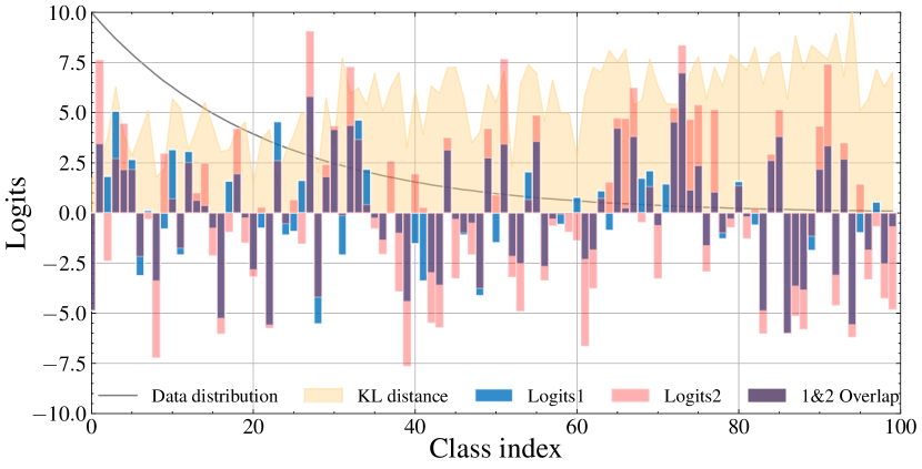
Figure 1: The comparisons of model outputs (logits) and Kullback–Leibler (KL) distance between two networks that are trained from scratch. Analysis is conducted on CIFAR100-LT dataset with Imbalanced Factor (IF) of 100. The logits are visualized on the basis of a random selected example, and the KL distance is computed based on the whole test set and then the average results of each category are counted and reported. Although the employed two networks have the same network structure and training settings, their predictions differ largely from each other especially in tail classes. Bested viewed in color.

In recent years, deep neural networks have achieved resounding success in various visual tasks, i.e., face analysis [47, 61], action and gesture recognition [65, 39]. Despite the advances in deep technologies and computing capability, the huge success also highly depends on large well-designed datasets of having a roughly balanced distribution, such as ImageNet [12], MS COCO [35] and Places [64]. This differs notably from real-world datasets, which usually exhibit long-tailed data distributions [51, 37] where few head classes occupy most of the data while many tail classes have only few samples. In such scenarios, the model is easily dominated by those few head classes, whereas low accuracy rates are usually achieved for many other tail classes. Undoubtedly, the long-tailed characteristics challenges deep visual recognition, and also immensely hinders the practical use of deep models.

In long-tailed visual recognition, several works focus on designing the class re-balancing strategies [44, 45, 17, 11, 24, 51] and decoupled learning [27, 4]. More recent efforts aim to improve the long-tailed learning by using multiple experts [53, 50, 33, 2, 58]. The multi-expert algorithms follow a straightforward idea of complementary learning, which means that different experts focus on different aspects and each of them benefits from the specialization in the dominating part. For example, LFME [53] formulates a network with three experts and it forces each expert learn samples from one of head, middle and tail classes. Previous multi-expert methods [50, 53, 2], however, only force each expert to learn the knowledge in a specific area, and there is a lack of cooperation among them.

Our motivation is inspired by a simple experiment as shown in Fig. 1, where the different networks vary considerably, particularly in tail classes, even if they have the same network structure and the same training settings. This signifies the great uncertainty in the learning process. One reliable solution to alleviate the uncertainty is the collaborative learning through multiple experts, namely, that each expert can be a teacher to others and also can be a student to learn additional knowledge of others. Grounded in this, we propose a Nested Collaborative Learning (NCL) for long-tailed visual recognition. NCL contains two main important components, namely Nested Individual Learning (NIL) and Nested Balanced Online Distillation (NBOD), the former of which aims to enhance the discriminative capability of each network, and the later collaboratively transfers the knowledge among any two experts. Both NCL and NBOD are performed in a nested way, where the NCL or NBOD conducts the supervised learning or distillation from a full perspective on all categories, and also implements that from a partial perspective of focusing on some important categories. Moreover, we propose a Hard Category Mining (HCM) to select the hard categories as the important categories, in which the hard category is defined as the category that is not the ground-truth category but with a high predicted score and easily resulting to misclassification. The learning manners from different perspectives are nested, related and complementary, which facilitates to the thorough representations learning. Furthermore, inspired by self-supervised learning [18], we further employ an additional moving average model for each expert to conduct self-supervision, which enhances the feature learning in an unsupervised manner.

In the proposed NCL, each expert is collaboratively learned with others, where the knowledge transferring between any two experts is allowed. NCL promotes each expert model to achieve better and even comparable performance to an ensemble’s. Thus, even if a single expert is used, it can be competent for prediction. Our contributions can be summarized as follows:

• We propose a Nested Collaborative Learning (NCL) to collaboratively learn multiple experts concurrently, which allows each expert model to learn extra knowledge from others.

• We propose a Nested Individual Learning (NIL) and Nested Balanced Online Distillation (NBOD) to conduct the learning from both a full perspective on all categories and a partial perspective of focusing on hard categories.

• We propose a Hard Category Mining (HCM) to greatly reduce the confusion with hard negative categories.

• The proposed method gains significant performance over the state-of-the-art on five popular datasets including CIFAR-10/100-LT, Places-LT, ImageNet-LT and iNaturalist 2018.

2 Related Work

Long-tailed visual recognition. To alleviate the long-tailed class imbalance, lots of studies  [63, 3, 53, 41, 50, 55, 36] are conducted in recent years. The existing methods for long-tailed visual recognition can be roughly divided into three categories: class re-balancing [17, 1, 11, 24, 42, 51], multi-stage training [27, 4] and multi-expert methods [53, 50, 33, 2, 58]. Class re-balancing, which aims to re-balance the contribution of each class during training, is a classic and widely used method for long-tailed learning. More specifically, class re-balancing consists of data re-sampling [5, 27], loss re-weighting [34, 48, 41, 43]. Class re-balancing improves the overall performance but usually at the sacrifice of the accuracy on head classes. Multi-stage training methods divide the training process into several stages. For example, Kang et al. [27] decouple the training procedure into representation learning and classifier learning. Li et al. [31] propose a multi-stage training strategy constructed on basis of knowledge distillation. Besides, some other works [38, 57] tend to improve performance via a post-process of shifting model logits. However, multi-stage training methods may rely on heuristic design. More recently, multi-expert frameworks receive increasing concern, e.g., LFME [53], BBN [63], RIDE [50], TADE [58] and ACE [2]. Multi-expert methods indeed improve the recognition accuracy for long-tailed learning, but those methods still need to be further exploited. For example, most current multi-expert methods employ different models to learn knowledge from different aspects, while the mutual supervision among them is deficient. Moreover, they often employ an ensemble of experts to produce predictions, which leads to a complexity increase of the inference phase.

Knowledge distillation. Knowledge distillation is a prevalent technology in knowledge transferring. Early methods [22, 40] often adopt an offline learning strategy, where the distillation follows a teacher-student learning scheme [22, 14], which transfers knowledge from a large teacher model to a small student model. However, the teacher normally should be a complex high-capacity model and the training process may be cumbersome and time-consuming. In recent years, knowledge distillation has been extended to an online way [60, 16, 6, 13], where the whole knowledge distillation is conducted in a one-phase and end-to-end training scheme. For example, in Deep Mutual Learning [60], any one model can be a student and can distil knowledge from all other models. Guo et al. [16] propose to use an ensemble of soft logits to guide the learning. Zhu et al. [30] propose a multi-branch architecture with treating each branch as a student to further reduce computational cost. Online distillation is an efficient way to collaboratively learn multiple models, and facilitates the knowledge transferred among them.

Contrastive learning. Many contrastive methods [18, 8, 7, 15] are built based on the task of instance discrimination. For example, Wu et al. [52] propose a noise contrastive estimation to compare instances based on a memory bank of storing representations. Representation learning for long-tailed distribution also been exploit [26]. More recently, Momentum Contrast (MoCo) [18] is proposed to produce the compared representations by a moving-averaged encoder. To enhance the discriminative ability, contrastive learning often compares each sample with many negative samples. SimCLR [7] achieves this by using a large batch size. Later, Chen et al. [8] propose an improved method named MOCOv2, which achieving promising performance without using a large batch size for training. Considering the advantages of MoCOv2, our self-supervision is also constructed based on this structure.

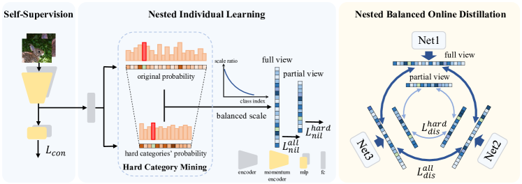
Figure 2: An illustration of our proposed NCL of containing three experts. The NIL enhances discriminative ability of a single expert, and NBOD allows knowledge transferring among multiple experts. NIL conducts the supervised learning from both a full and a partial view, which focus on all categories and some hard categories, respectively. Similarly, NBOD conducts the knowledge distillation also from both a full and a partial view. The contrastive loss is calculated by using an extra momentum encoder and MLP layers, which can be removed in evaluation. Probabilities employed in NIL and NBOD are balanced according to the data distribution.

3 Methodology

The proposed NCL aims to collaboratively and concurrently learn multiple experts together as shown in Fig. 2. In the following, firstly, we introduce the preliminaries, and then present Hard Category Mining (HCM), Nested Individual Learning (NIL), Nested Balanced Online Distillation (NBOD) and self-supervision part. Finally, we show the overall loss of how to aggregate them together.

3.1 Preliminaries

We denote the training set with $n$ samples as ${{\mathcal{D}}}=\{{\bf x}_{i},y_{i}\}$, where ${\bf x}_{i}$ indicates the $i$-th image sample and $y_{i}$ denotes the corresponding label. Assume a total of $K$ experts are employed and the $k$-th expert model is parameterized with ${\bm{\theta}}_{k}$. Given image ${\bf x}_{i}$, the predicted probability of class-$j$ in the $k$-th expert is computed as:

$${\tilde{\bf p}}_{j}({\bf x}_{i};{\bm{\theta}}_{k})=\frac{exp({{z}_{ij}^{k}})}{\sum_{l=1}^{C}exp({{z}_{il}^{k}})}$$ (1)

where $z_{ij}^{k}$ is the k-th expert model’s class-$j$ output and $C$ is the number of classes. This is a widely used way to compute the predicted probability, and some losses like Cross Entropy (CE) loss is computed based on it. However, it does not consider the data distribution, and is not suitable for long-tailed visual recognition, where a naive learned model based on ${\tilde{\bf p}}({\bf x}_{i};{\bm{\theta}}_{k})$ would be largely dominated by head classes. Therefore, some researchers [41] proposed to compute predicted probability of class-$j$ in a balanced way:

$${\bf p}_{j}({\bf x}_{i};{\bm{\theta}}_{k})=\frac{n_{j}exp({{z}_{ij}^{k}})}{\sum_{l=1}^{C}n_{l}exp({{z}_{il}^{k}})}$$ (2)

where $n_{j}$ is the total number of samples of class $j$. In this way, contributions of tail classes are strengthened while contributions of head classes are suppressed. Based on such balanced probabilities, Ren et al. [41] further proposed a Balanced Softmax Cross Entropy (BSCE) loss to alleviate long-tailed class imbalance in model training. However, BSCE loss is still not enough, where the uncertainty in training still cannot be eliminated.

3.2 Hard Category Mining

In representation learning, one well-known and effective strategy to boost performance is Hard Example Mining (HEM) [21]. HEM selects hard samples for training while discarding easy samples. However, directly applying HEM to long-tailed visual recognition may distort the data distribution and make it more skewed in long-tailed learning. Differing from HEM, we propose a more amicable method named Hard Category Mining (HCM) to exclusively select hard categories for training, which explicitly improves the ability of distinguishing the sample from hard categories. In HCM, the hard category means the category that is not the ground-truth category but with a high predicted score. Therefore, the hard categories can be selected by comparing values of model’s outputs. Specifically, we have $C$ categories in total and suppose $C_{hard}$ categories are selected to focus on. For the sample ${\bf x}_{i}$ and expert $k$, the corresponding set ${\bm{\Psi}}_{i}^{k}$ containing the output of selected categories is denoted as:

$${\bm{\Psi}}_{i}^{k}=TopHard\{z_{ij}^{k}|j\neq y_{i}\}\cup\{z_{iy_{i}}^{k}\}$$ (3)

where $TopHard$ means selecting $C_{hard}$ examples with largest values. In order to adapt to long-tailed learning better, we computed the probabilities of the selected categories in a balanced way, which is shown as:

$${\bf p}^{*}({\bf x}_{i};{\bm{\theta}}_{k})=\{\frac{n_{j}exp({{z}_{ij}^{k}})}{\sum_{z_{il}^{k}\in{\bm{\Psi}}_{i}^{k}}n_{l}exp({{z}_{il}^{k}})}|{z}_{ij}^{k}\in{\bm{\Psi}}_{i}^{k}\}$$ (4)

3.3 Nested Individual Learning

The individual supervised learning on each expert is also an important component in our NCL, which ensures that each network can achieve the strong discrimination ability. To learn thoroughly, we proposed a Nested Individual Learning (NIL) to perform the supervision in a nested way. Besides the supervision on all categories for a global and robust learning, we also force the network to focus on some important categories selected by HCM, which enhance model’s meticulous distinguishing ability. The supervision on all categories is trivial and constructed on BSCE loss. Since our framework is constructed on multiple experts, the supervision is applied to each expert and the loss on all categories over all experts is the sum of the loss of each expert:

$$L_{nil}^{all}=-\textstyle{\sum\nolimits_{k}}log({{\bf p}}_{y_{i}}({\bf x}_{i};{\bm{\bm{\theta}}}_{k}))$$ (5)

For the supervision on hard categories, it also can be obtained in a similar way. Mathematically, it can be represented as:

$$L_{nil}^{hard}=-\textstyle{\sum\nolimits_{k}}log({{\bf p}^{*}}_{y_{i}}({\bf x}_{i};{\bm{\bm{\theta}}}_{k}))$$ (6)

In the proposed NIL, the two nested supervisions are employed together to achieve a comprehensive learning, and the summed loss is written as:

$$L_{nil}=L_{nil}^{all}+L_{nil}^{hard}$$ (7)

3.4 Nested Balanced Online Distillation

To collaboratively learn multiple experts from each other, online distillation is employed to allow each model to learn extra knowledge from others. Previous methods [60, 16] consider the distillation from a full perspective of all categories, which aims to capture global and robust knowledge. Different from previous methods, we propose a Nested Balanced Online Distillation (NBOD), where the distillation is conducted not only on all categories, but also on some hard categories that are mined by HCM, which facilitates the network to capture meticulous distinguishing ability. According to previous works [60, 16], the Kullback Leibler (KL) divergence is employed to perform the knowledge distillation. The distillation on all categories can be formulated as:

$$L_{dis}^{all}=\frac{1}{K(K-1)}{\sum_{k}^{K}\sum_{q\neq k}^{K}}KL({\bf p}({\bf x}_{i};{\bm{\theta}}_{k})||{\bf p}({\bf x}_{i};{\bm{\theta}}_{q}))$$ (8)

As we can see, the distillation is conducted among any two experts. Note here that we use balanced distributions instead of original distributions to compute KL distance, which aims to eliminate the distribution bias under the long-tailed setting. And this is also one aspect of how we distinguish from other distillation methods. Moreover, all experts employ the same hard categories for distillation, and we randomly select an expert as an anchor to generate hard categories for all experts. Similarly, the distillation on hard categories also can be formulated as:

$$L_{dis}^{hard}=\frac{1}{K(K-1)}{\sum_{k}^{K}\sum_{q\neq k}^{K}}KL({\bf p}^{*}({\bf x}_{i};{\bm{\theta}}_{k})||{\bf p}^{*}({\bf x}_{i};{\bm{\theta}}_{q}))$$ (9)

The nested distillation on both all categories and hard categories are learned together, which is formulated as:

$$L_{dis}=L_{dis}^{all}+L_{dis}^{hard}$$ (10)

3.5 Feature Enhancement via Self-Supervision

Self-supervised learning aims to improve feature representations via an unsupervised manner. Following previous works [18, 8], we adopt the instance discrimination as the self-supervised proxy task, in which each image is regarded as a distinct class. We leverage an additional temporary average model so as to conduct self-supervised learning, and its parameters are updated following a momentum-based moving average scheme [18, 8] as shown in Fig. 2. The employed self-supervision is also a part of our NCL, which cooperatively learns an expert model and its moving average model to capture better features.

Take the self-supervision for expert $k$ as an example. Let ${\bf v}_{i}^{k}$ denote the normalized embedding of the $i^{th}$ image in the original expert model, and ${\bf{\tilde{v}}}_{i}^{k}$ denote the normalized embedding of its copy image with different augmentations in the temporally average model. Besides, a dynamic queue $\mathcal{Q}^{k}$ is employed to collect historical features. The samples in the queue are progressively replaced with the samples in current batch enqueued and the samples in oldest batch dequeued. Assume that the queue $\mathcal{Q}^{k}$ has a size of $N$ and $N$ can be set to be much larger than the typical batch size, which provides a rich set of negative samples and thus obtains better feature representations. The goal of instance discrimination task is to increase the similarity of features of the same image while reduce the similarity of the features of two different images. We achieve this by using a contrastive learning loss, which is computed as:

$$L_{con}^{k}=-log(\frac{exp({{\bf v}_{i}^{k}}^{T}{\bf{\tilde{v}}}_{i}^{k}/\tau)}{exp({{\bf v}_{i}^{k}}^{T}{\bf{\tilde{v}}}_{i}^{k}/\tau)+\sum_{{\bf{\tilde{v}}}_{j}^{k}\in{\mathcal{Q}^{k}}}exp({{\bf v}_{i}^{k}}^{T}{\bf{\tilde{v}}}_{j}^{k}/\tau)})$$ (11)

where $\tau$ is a temperature hyper-parameter. Similar to Eq. 5 and Eq. 6, the self-supervised loss over all experts can be represented as $L_{con}=\sum\nolimits_{k}L_{con}^{k}$.

3.6 Model Training

The overall loss in our proposed NCL consists of three parts: the loss $L_{nil}$ of our NIL for learning each expert individually, the loss $L_{dis}$ of our NBOD for cooperation among multiple experts, and the loss $L_{con}$ of self-supervision. The overall loss $L$ is formulated as:

$$L=L_{nil}+L_{con}+\lambda L_{dis}$$ (12)

where $\lambda$ denotes the loss weight to balance the contribution of cooperation among multiple experts. For $L_{nil}$ and $L_{con}$, they play their part inside the single expert, and we equally set their weighs as 1 in consideration of generality.

4 Experiments

4.1 Datasets and Protocols

We conduct experiments on five widely used datasets, including CIFAR10-LT [11], CIFAR100-LT [11], ImageNet-LT [37], Places-LT [64], and iNaturalist 2018 [46].

CIFAR10-LT and CIFAR100-LT [11] are created from the original balanced CIFAR datasets [29]. Specifically, the degree of data imbalance in datasets is controlled by an Imbalance Factor (IF), which is defined by dividing the number of the most frequent category by that of the least frequent category. The imbalance factors of 100 and 50 are employed in these two datasets. ImageNet-LT [37] is sampled from the popular ImageNet dataset [12] under long-tailed setting following the Pareto distribution with power value $\alpha$=6. ImageNet-LT contains 115.8K images from 1,000 categories. Places-LT is created from the large-scale dataset Places [64]. This dataset contains 184.5K images from 365 categories. iNaturalist 2018 [46] is the largest dataset for long-tailed visual recognition. iNaturalist 2018 contains 437.5K images from 8,142 categories, and it is extremely imbalanced with an imbalance factor of 512.

According to previous works [11, 27] the top-1 accuracy is employed for evaluation. Moreover, for iNaturalist 2018 dataset, we follow the works [2, 27] to divide classes into many (with more than 100 images), medium (with 20 $\sim$ 100 images) and few (with less than 20 images) splits, and further report the results on each split.

4.2 Implementation Details

For CIFAR10/100-LT, following [4, 59], we adopt ResNet-32 [19] as our backbone network and liner classifier for all the experiments. We utilize ResNet-50 [19], ResNeXt-50 [54] as our backbone network for ImageNet-LT, ResNet-50 for iNaturalist 2018 and pretrained ResNet-152 for Places-LT respectively, based on [37, 27, 10]. Following [57], cosine classifier is utilized for these models. Due to the use of the self-supervision component, we use the same training strategies as PaCo [10], i.e., training all the models for 400 epochs except models on Places-LT, which is 30 epochs. In addition, for fair comparison, following [10], RandAugument [9] is also used for all the experiments except Places-LT. The influence of RandAugument will be discussed in detail in Sec. 4.4. These models are trained on 8 NVIDIA Tesla V100 GPUs.

The $\beta=C_{hard}/C$ in HCM is set to 0.3. And the ratio of Nested Balanced Online Distillation loss $\lambda$, which plays its part among networks, is set to 0.6. The influence of $\beta$ and $\lambda$ will be discussed in detail in Sec. 4.4.

Method	Ref.	CIFAR100-LT		CIFAR10-LT
		100	50	100	50
CB Focal loss [11]	CVPR’19	38.7	46.2	74.6	79.3
LDAM+DRW [4]	NeurIPS’19	42.0	45.1	77.0	79.3
LDAM+DAP [25]	CVPR’20	44.1	49.2	80.0	82.2
BBN [63]	CVPR’20	39.4	47.0	79.8	82.2
LFME [53]	ECCV’20	42.3	–	–	–
CAM [59]	AAAI’21	47.8	51.7	80.0	83.6
Logit Adj. [38]	ICLR’21	43.9	–	77.7	–
RIDE [50]	ICLR’21	49.1	–	–	–
LDAM+M2m [28]	CVPR’21	43.5	–	79.1	–
MiSLAS [62]	CVPR’21	47.0	52.3	82.1	85.7
LADE [23]	CVPR’21	45.4	50.5	–	–
Hybrid-SC [49]	CVPR’21	46.7	51.9	81.4	85.4
DiVE [20]	ICCV’21	45.4	51.3	–	–
SSD [32]	ICCV’21	46.0	50.5	–	–
ACE [2]	ICCV’21	49.6	51.9	81.4	84.9
PaCo [10]	ICCV’21	52.0	56.0	–	–
BSCE (baseline)	–	50.6	55.0	84.0	85.8
Ours (single)	–	53.3	56.8	84.7	86.8
Ours (ensemble)	–	54.2	58.2	85.5	87.3

Table 1: Comparisons on CIFAR100-LT and CIFAR10-LT datasets with the IF of 100 and 50.

Method	Ref.	ImageNet-LT		Places-LT
		Res50	ResX50	Res152
OLTR [37]	CVPR’19	–	–	35.9
BBN [63]	CVPR’20	48.3	49.3	–
NCM [27]	ICLR’20	44.3	47.3	36.4
cRT [27]	ICLR’20	47.3	49.6	36.7
$\tau$-norm [27]	ICLR’20	46.7	49.4	37.9
LWS [27]	ICLR’20	47.7	49.9	37.6
BSCE [41]	NeurIPS’20	–	–	38.7
RIDE [50]	ICLR’21	55.4	56.8	–
DisAlign [57]	CVPR’21	52.9	–	–
DiVE [20]	ICCV’21	53.1	–	–
SSD [32]	ICCV’21	–	56.0	–
ACE [2]	ICCV’21	54.7	56.6	–
PaCo [10]	ICCV’21	57.0	58.2	41.2
BSCE (baseline)	–	53.9	53.6	40.2
Ours (single)	–	57.4	58.4	41.5
Ours (ensemble)	–	59.5	60.5	41.8

Table 2: Comparisons on ImageNet-LT and Places-LT datasets.

Method	Ref.	iNaturalist 2018
		Many	Medium	Few	All
OLTR [37]	CVPR’19	59.0	64.1	64.9	63.9
BBN [63]	CVPR’20	49.4	70.8	65.3	66.3
DAP [25]	CVPR’20	–	–	–	67.6
NCM [27]	ICLR’20
cRT [27]	ICLR’20	69.0	66.0	63.2	65.2
$\tau$-norm [27]	ICLR’20	65.6	65.3	65.9	65.6
LWS [27]	ICLR’20	65.0	66.3	65.5	65.9
LDAM+DRW [4]	NeurIPS’19	–	–	–	68.0
Logit Adj. [38]	ICLR’21	–	–	–	66.4
CAM [59]	AAAI’21	–	–	–	70.9
RIDE [50]	ICLR’21	70.9	72.4	73.1	72.6
SSD [32]	ICCV’21
ACE [2]	ICCV’21	–	–	–	72.9
PaCo [10]	ICCV’21	–	–	–	73.2
BSCE (baseline)	–	67.5	72.0	71.5	71.6
Ours (single)	–	72.0	74.9	73.8	74.2
Ours(ensemble)	–	72.7	75.6	74.5	74.9

Table 3: Comparisons on iNaturalist 2018 dataset with ResNet-50.

4.3 Comparisons to Prior Arts

We compare the proposed method NCL with previous state-of-the-art methods, like LWS [27], ACE [2] and so on. Our NCL is constructed based on three experts and both the performance of a single expert and an ensemble of multiple experts are reported. Besides NCL, we also report the baseline results of a network with using BSCE loss for comparisons. Comparisons on CIFAR10/100-LT are shown in Table 1, comparisons on ImageNet-LT and Places-LT are shown in Table 2, and comparisons on iNaturalist2018 are shown in Table 3. Our proposed method achieves the state-of-the-art performance on all datasets whether using a single expert or an ensemble of all experts. For only using a single expert for evaluation, our NCL outperforms previous methods on CIFAR10-LT, CIFAR100-LT, ImageNet-LT, Places-LT and iNaturalist2018 with accuracies of 84.7% (IF of 100), 53.3% (IF of 100), 57.4% (with ResNet-50), 41.5% and 74.2%, respectively. When further using an ensemble for evaluation, the performance on CIFAR10-LT, CIFAR100-LT, ImageNet-LT, Places-LT and iNaturalist2018 can be further improved to 85.5% (IF of 100), 54.2% (IF of 100), 59.5% (with ResNet-50), 41.8% and 74.9%, respectively. More results on many, medium and few splits are listed in Supplementary Material. Some previous multi-expert methods were constructed based on a multi-branch network with higher complexity. For example, RIDE [50] with 4 experts brings 0.4 times more computation than the original single network. However, our method of only using a single expert for evaluation won’t bring any extra computation but still outperforms them. Besides, despite that some previous methods employ a multi-stage training [32, 27] or a post-processing [38, 57] to further improve the performance, our method still outperforms them. The significant performance over the state-of-the-art shows the effectiveness of our proposed NCL.

4.4 Component Analysis

Influence of the ratio of hard categories. The ratio of selected hard categories is defined as $\beta=C_{hard}/C$. Experiments on our NIL model are conducted within the range of $\beta$ from 0 to 1 as shown in Fig. 3 (a). The highest performance is achieved when setting $\beta$ to 0.3. Setting $\beta$ with a small and large values brings limited gains due to the under and over explorations on hard categories.

Effect of loss weight. To search an appropriate value for $\lambda$, experiments on the proposed NCL with a series of $\lambda$ are conducted as shown in Fig. 3 (b). $\lambda$ controls the contribution of knowledge distillation among multiple experts in total loss. The best performance is achieved when $\lambda=0.6$, which shows that a balance is achieved between single network training and knowledge transferring among experts.

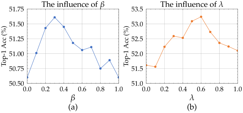
Figure 3: Parameter analysis of (a) the ratio $\beta$ and (b) the loss weight $\lambda$ on CIFAR100-LT dataset with IF of 100.

Impact of different number of experts. As shown in Fig. 4, experiments using different number of experts are conducted. The ensemble performance is improved steadily as the number of experts increases, while for only using a single expert for evaluation, its performance can be greatly improved when only using a small number of expert networks, e.g., three experts. Therefore, three experts are mostly employed in our multi-expert framework for a balance between complexity and performance.

Single expert vs. multi-expert. Our method is essentially a multi-expert framework, and the comparison among using a single expert or an ensemble of multi-expert is a matter of great concern. As shown in Fig. 4, As the number of experts increases, the accuracy of the ensemble over a single expert also tends to rise. This demonstrates the power of ensemble learning. But for the main goal of our proposed NCL, the performance improvement over a single expert is impressive enough at the number of three.

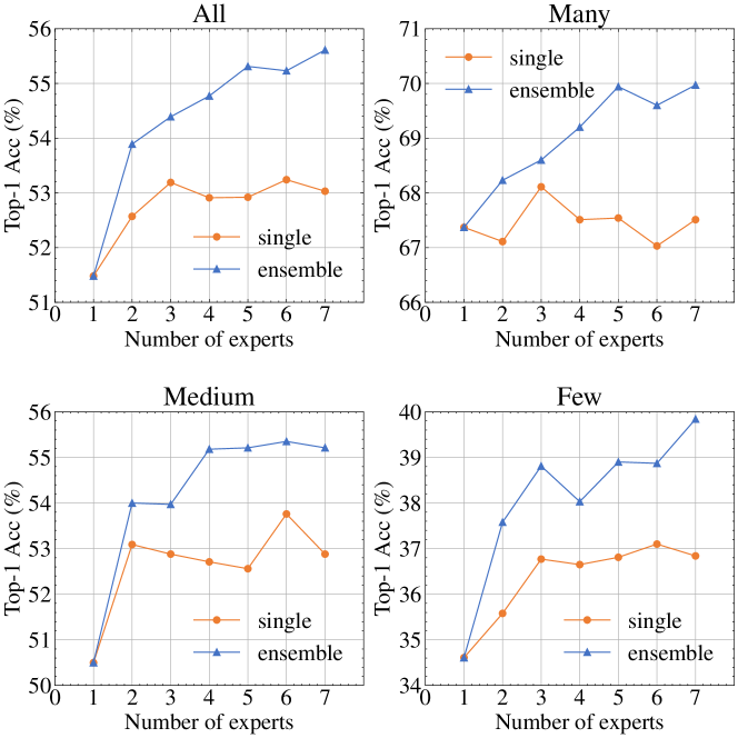
Figure 4: Comparisons of using different expert numbers on CIFAR100-LT with an IF of 100. We report the performance on both a single network and an ensemble. Specifically, the performance on a single network is reported as the average accuracy on all experts, and the ensemble performance is computed based on the averaging logits over all experts.

Influence of data augmentations. Data augmentation is a common tool to improve performance. For example, previous works use Mixup [59, 2, 62, 56] and RandAugment [9] to obtain richer feature representations. Our method follows PaCo [10] to employ RandAugment [9] for experiments. As shown in Table 4, the performance is improved by about 3% to 5% when employing RandAugment for training. However, our high performance depends not entirely on RandAugment. When dropping RandAugment, our ensemble model reaches an amazing performance of 49.22%, which achieves comparable performance to the current state-of-the-art ones.

Method	w/o RandAug	w/ RandAug
CE	41.88	44.79
BSCE	45.88	50.60
BSCE+NCL	47.93	53.31
BSCE+NCL†	49.22	54.42

Table 4: Comparisons of training the network with (’w/’) and without (’w/o’) employing RandAugment. Experiments are conducted on CIFAR100-LT dataset with an IF of 100. ^† Indicates the ensemble performance is reported.

Ablation studies on all components. In this sub-section, we perform detailed ablation studies for our NCL on CIFAR100-LT dataset, which is shown in Table 5. To conduct a comprehensive analysis, we evaluate the proposed components including Self-Supervision (’SS’ for short), NIL, NBOD and ensemble on two baseline settings of using CE and BSCE losses. Furthermore, for more detailed analysis, we split NBOD into two parts namely BOD_all and BOD_hard. Take the BSCE setting as an example, SS and NIL improve the performance by 0.82% and 0.64%, respectively. And employing NBOD further improves the performance from 51.24% to 53.19%. When employing an ensemble for evaluation, the accuracy is further improved and reaches the highest. For the CE baseline setting, similar improvements can be achieved for SS, NIL, DBOD and ensemble. Generally, benefiting from the label distribution shift, BSCE loss can achieve better performance than CE loss. The steadily performance improvements are achieved for all components on both baseline settings, which shows the effectiveness of the proposed NCL.

NIL	SS	BODall	BODhard	Ensemble	Acc.@CE	Acc.@BSCE
					44.79	50.60
✓					48.18	51.24
	✓				46.05	51.42
✓		✓			48.81	52.64
✓		✓	✓		49.34	53.19
✓	✓	✓	✓		49.89	53.31
✓	✓	✓	✓	✓	51.04	54.42

Table 5: Ablation studies on CIFAR100-LT dataset with an IF of 100. ’SS’ indicates self-supervision. ’BOD_all’ and ’BOD_hard’ represent the balanced online distillation on all categories and only hard categories, respectively. NBOD means the setting when both ’BOD_all’ and ’BOD_hard’ are employed. Experiments are conducted on the framework of containing three experts.

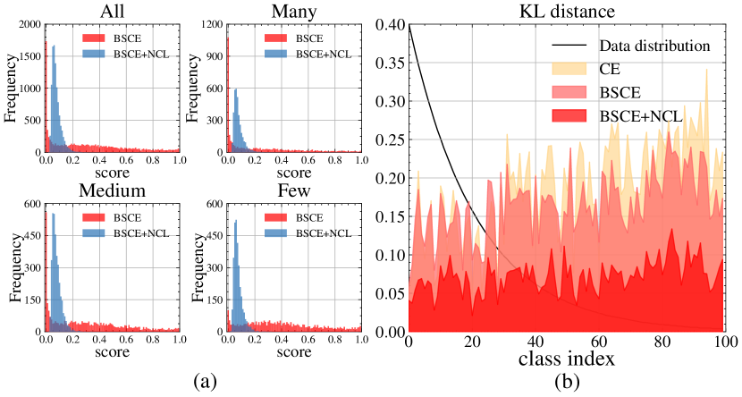
Figure 5: (a) The distribution of the largest softmax probability of hardest negative category. (b) The average KL distance between two models’ output probabilities on the test set. Analysis is conducted on CIFAR100-LT with an IF of 100. Best viewed in color.

4.5 Discussion and Further Analysis

Score distribution of hardest negative category. Deep models normally confuse the target sample with the hardest negative category. Here we visualize the score distribution for the baseline method (’BSCE’) and our method (’BSCE+NCL’) as shown in Fig 5 (a). The higher the score of the hardest negative category is, the more likely it is to produce false recognition. The scores in our proposed method are mainly concentrated in the range of 0-0.2, while the scores in the baseline model are distributed in the whole interval (including the interval with large values). This shows that our NCL can considerably reduce the confusion with the hardest negative category.

KL distance of pre/post collaborative learning. As shown in Fig. 5 (b), when networks are trained with our NCL, the KL distance between them is greatly reduced, which shows that the uncertainty in predictions is effectively alleviated. Besides, the KL distance is more balanced than that of BSCE and CE, which indicates that collaborative learning is of help to the long-tailed bias reduction.

NBOD without balancing probability. As shown in Fig. 6 (a), when removing the balanced probability in NBOD (denoted as ’NOD’) both the performance of the single expert and the ensemble decline about 1%, which manifests the importance of employing the balanced probability for the distillation in long-tailed learning.

Offline distillation vs. NBOD. To further verify the effectiveness of our NBOD, we employ an offline distillation for comparisons. The offline distillation (denoted as ’NIL+OffDis’) first employs three teacher networks of NIL to train individually, and then produces the teacher labels by using the averaging outputs over three teacher models. The comparisons are shown in Fig. 6 (b). Although NIL+OffDis gains some improvements via an offline distillation, but its performance still 1.5% worse than that of NIL+NBOD. It shows that our NBOD of the collaborative learning can learn more knowledge than offline distillation.

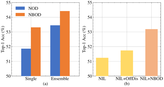
Figure 6: (a) Comparisons of using NOD or NBOD for distillation. (b) Comparisons of using offline distillation or our NBOD. Analysis is conducted on CIFAR100-LT with an IF of 100.

5 Conclusions

In this work, we have proposed a Nested Collaborative Learning (NCL) to collaboratively learn multiple experts. Two core components, i.e., NIL and NBOD, are proposed for individual learning of a single expert and knowledge transferring among multiple experts. Both NIL and NBOD consider the features learning from both a full perspective and a partial perspective, which exhibits in a nested way. Moreover, we have proposed a HCM to capture hard categories for learning thoroughly. Extensive experiments have verified the superiorities of our method.

Limitations and Broader impacts. One limitation is that more GPU memory and computing power are needed when training our NCL with multiple experts. But fortunately, one expert is also enough to achieve promising performance in inference. Moreover, the proposed method improves the accuracy and fairness of the classifier, which promotes the visual model to be further put into practical use. To some extent, it helps to collect large datasets without forcing class balancing preprocessing, which improves efficiency and effectiveness of work. The negative impacts can yet occur in some misuse scenarios, e.g., identifying minorities for malicious purposes. Therefore, the appropriateness of the purpose of using long-tailed classification technology is supposed to be ensured with attention.

References

- [1] Mateusz Buda, Atsuto Maki, and Maciej A Mazurowski. A systematic study of the class imbalance problem in convolutional neural networks. Neural Networks, 2018.
- [2] Jiarui Cai, Yizhou Wang, and Jenq-Neng Hwang. Ace: Ally complementary experts for solving long-tailed recognition in one-shot. In ICCV, 2021.
- [3] Dong Cao, Xiangyu Zhu, Xingyu Huang, Jianzhu Guo, and Zhen Lei. Domain balancing: Face recognition on long-tailed domains. In CVPR, 2020.
- [4] Kaidi Cao, Colin Wei, Adrien Gaidon, Nikos Arechiga, and Tengyu Ma. Learning imbalanced datasets with label-distribution-aware margin loss. In NeurIPS, 2019.
- [5] Nitesh V Chawla, Kevin W Bowyer, Lawrence O Hall, and W Philip Kegelmeyer. Smote: synthetic minority over-sampling technique. Journal of artificial intelligence research, 16:321–357, 2002.
- [6] Defang Chen, Jian-Ping Mei, Can Wang, Yan Feng, and Chun Chen. Online knowledge distillation with diverse peers. In AAAI, 2020.
- [7] Ting Chen, Simon Kornblith, Mohammad Norouzi, and Geoffrey Hinton. A simple framework for contrastive learning of visual representations. In ICML, 2020.
- [8] Xinlei Chen, Haoqi Fan, Ross Girshick, and Kaiming He. Improved baselines with momentum contrastive learning. arXiv preprint arXiv:2003.04297, 2020.
- [9] Ekin D Cubuk, Barret Zoph, Jonathon Shlens, and Quoc V Le. Randaugment: Practical automated data augmentation with a reduced search space. In CVPRW, 2020.
- [10] Jiequan Cui, Zhisheng Zhong, Shu Liu, Bei Yu, and Jiaya Jia. Parametric contrastive learning. In ICCV, 2021.
- [11] Yin Cui, Menglin Jia, Tsung-Yi Lin, Yang Song, and Serge Belongie. Class-balanced loss based on effective number of samples. In CVPR, 2019.
- [12] Jia Deng, Wei Dong, Richard Socher, Li-Jia Li, Kai Li, and Li Fei-Fei. Imagenet: A large-scale hierarchical image database. In CVPR, 2009.
- [13] Nikita Dvornik, Cordelia Schmid, and Julien Mairal. Diversity with cooperation: Ensemble methods for few-shot classification. In ICCV, 2019.
- [14] Tommaso Furlanello, Zachary Lipton, Michael Tschannen, Laurent Itti, and Anima Anandkumar. Born again neural networks. In ICML, 2018.
- [15] Jean-Bastien Grill, Florian Strub, Florent Altché, Corentin Tallec, Pierre H Richemond, Elena Buchatskaya, Carl Doersch, Bernardo Avila Pires, Zhaohan Daniel Guo, Mohammad Gheshlaghi Azar, et al. Bootstrap your own latent: A new approach to self-supervised learning. arXiv preprint arXiv:2006.07733, 2020.
- [16] Qiushan Guo, Xinjiang Wang, Yichao Wu, Zhipeng Yu, Ding Liang, Xiaolin Hu, and Ping Luo. Online knowledge distillation via collaborative learning. In CVPR, 2020.
- [17] Haibo He and Edwardo A Garcia. Learning from imbalanced data. IEEE TKDE, 2009.
- [18] Kaiming He, Haoqi Fan, Yuxin Wu, Saining Xie, and Ross Girshick. Momentum contrast for unsupervised visual representation learning. In CVPR, 2020.
- [19] Kaiming He, Xiangyu Zhang, Shaoqing Ren, and Jian Sun. Deep residual learning for image recognition. In CVPR, 2016.
- [20] Yin-Yin He, Jianxin Wu, and Xiu-Shen Wei. Distilling virtual examples for long-tailed recognition. In ICCV, 2021.
- [21] Alexander Hermans, Lucas Beyer, and Bastian Leibe. In defense of the triplet loss for person re-identification. arXiv preprint arXiv:1703.07737, 2017.
- [22] Geoffrey Hinton, Oriol Vinyals, and Jeff Dean. Distilling the knowledge in a neural network. arXiv preprint arXiv:1503.02531, 2015.
- [23] Youngkyu Hong, Seungju Han, Kwanghee Choi, Seokjun Seo, Beomsu Kim, and Buru Chang. Disentangling label distribution for long-tailed visual recognition. In CVPR, 2021.
- [24] Chen Huang, Yining Li, Chen Change Loy, and Xiaoou Tang. Learning deep representation for imbalanced classification. In CVPR, 2016.
- [25] Muhammad Abdullah Jamal, Matthew Brown, Ming-Hsuan Yang, Liqiang Wang, and Boqing Gong. Rethinking class-balanced methods for long-tailed visual recognition from a domain adaptation perspective. In CVPR, 2020.
- [26] Bingyi Kang, Yu Li, Sa Xie, Zehuan Yuan, and Jiashi Feng. Exploring balanced feature spaces for representation learning. In International Conference on Learning Representations, 2020.
- [27] Bingyi Kang, Saining Xie, Marcus Rohrbach, Zhicheng Yan, Albert Gordo, Jiashi Feng, and Yannis Kalantidis. Decoupling representation and classifier for long-tailed recognition. arXiv preprint arXiv:1910.09217, 2019.
- [28] Jaehyung Kim, Jongheon Jeong, and Jinwoo Shin. M2m: Imbalanced classification via major-to-minor translation. In CVPR, 2020.
- [29] Alex Krizhevsky, Geoffrey Hinton, et al. Learning multiple layers of features from tiny images. 2009.
- [30] Xu Lan, Xiatian Zhu, and Shaogang Gong. Knowledge distillation by on-the-fly native ensemble. arXiv preprint arXiv:1806.04606, 2018.
- [31] Tianhao Li, Limin Wang, and Gangshan Wu. Self supervision to distillation for long-tailed visual recognition. In ICCV, 2021.
- [32] Tianhao Li, Limin Wang, and Gangshan Wu. Self supervision to distillation for long-tailed visual recognition. In ICCV, 2021.
- [33] Yu Li, Tao Wang, Bingyi Kang, Sheng Tang, Chunfeng Wang, Jintao Li, and Jiashi Feng. Overcoming classifier imbalance for long-tail object detection with balanced group softmax. In CVPR, 2020.
- [34] Tsung-Yi Lin, Priya Goyal, Ross Girshick, Kaiming He, and Piotr Dollár. Focal loss for dense object detection. In ICCV, 2017.
- [35] Tsung-Yi Lin, Michael Maire, Serge Belongie, James Hays, Pietro Perona, Deva Ramanan, Piotr Dollár, and C Lawrence Zitnick. Microsoft coco: Common objects in context. In ECCV, 2014.
- [36] Jialun Liu, Jingwei Zhang, Wenhui Li, Chi Zhang, and Yifan Sun. Memory-based jitter: Improving visual recognition on long-tailed data with diversity in memory. In AAAI, 2022.
- [37] Ziwei Liu, Zhongqi Miao, Xiaohang Zhan, Jiayun Wang, Boqing Gong, and Stella X Yu. Large-scale long-tailed recognition in an open world. In CVPR, 2019.
- [38] Aditya Krishna Menon, Sadeep Jayasumana, Ankit Singh Rawat, Himanshu Jain, Andreas Veit, and Sanjiv Kumar. Long-tail learning via logit adjustment. arXiv preprint arXiv:2007.07314, 2020.
- [39] Sushmita Mitra and Tinku Acharya. Gesture recognition: A survey. IEEE Transactions on Systems, Man, and Cybernetics, Part C (Applications and Reviews), 2007.
- [40] Nikolaos Passalis and Anastasios Tefas. Learning deep representations with probabilistic knowledge transfer. In ECCV, 2018.
- [41] Jiawei Ren, Cunjun Yu, Shunan Sheng, Xiao Ma, Haiyu Zhao, Shuai Yi, and Hongsheng Li. Balanced meta-softmax for long-tailed visual recognition. arXiv preprint arXiv:2007.10740, 2020.
- [42] Mengye Ren, Wenyuan Zeng, Bin Yang, and Raquel Urtasun. Learning to reweight examples for robust deep learning. In ICML, 2018.
- [43] Jingru Tan, Changbao Wang, Buyu Li, Quanquan Li, Wanli Ouyang, Changqing Yin, and Junjie Yan. Equalization loss for long-tailed object recognition. In CVPR, 2020.
- [44] Zichang Tan, Jun Wan, Zhen Lei, Ruicong Zhi, Guodong Guo, and Stan Z Li. Efficient group-n encoding and decoding for facial age estimation. TPAMI, 40(11):2610–2623, 2017.
- [45] Zichang Tan, Yang Yang, Jun Wan, Hanyuan Hang, Guodong Guo, and Stan Z Li. Attention-based pedestrian attribute analysis. TIP, 28(12):6126–6140, 2019.
- [46] Grant Van Horn, Oisin Mac Aodha, Yang Song, Yin Cui, Chen Sun, Alex Shepard, Hartwig Adam, Pietro Perona, and Serge Belongie. The inaturalist species classification and detection dataset. In CVPR, 2018.
- [47] Jun Wan, Guodong Guo, Sergio Escalera, Hugo Jair Escalante, and Stan Z Li. Multi-modal face presentation attack detection. SLCV, 9(1):1–88, 2020.
- [48] Jiaqi Wang, Wenwei Zhang, Yuhang Zang, Yuhang Cao, Jiangmiao Pang, Tao Gong, Kai Chen, Ziwei Liu, Chen Change Loy, and Dahua Lin. Seesaw loss for long-tailed instance segmentation. In CVPR, 2021.
- [49] Peng Wang, Kai Han, Xiu-Shen Wei, Lei Zhang, and Lei Wang. Contrastive learning based hybrid networks for long-tailed image classification. In CVPR, 2021.
- [50] Xudong Wang, Long Lian, Zhongqi Miao, Ziwei Liu, and Stella X Yu. Long-tailed recognition by routing diverse distribution-aware experts. In ICLR, 2021.
- [51] Yu-Xiong Wang, Deva Ramanan, and Martial Hebert. Learning to model the tail. In NeurIPS, 2017.
- [52] Zhirong Wu, Yuanjun Xiong, Stella X Yu, and Dahua Lin. Unsupervised feature learning via non-parametric instance discrimination. In CVPR, 2018.
- [53] Liuyu Xiang, Guiguang Ding, and Jungong Han. Learning from multiple experts: Self-paced knowledge distillation for long-tailed classification. In ECCV, 2020.
- [54] Saining Xie, Ross Girshick, Piotr Dollár, Zhuowen Tu, and Kaiming He. Aggregated residual transformations for deep neural networks. In CVPR, 2017.
- [55] Han-Jia Ye, Hong-You Chen, De-Chuan Zhan, and Wei-Lun Chao. Identifying and compensating for feature deviation in imbalanced deep learning. arXiv preprint arXiv:2001.01385, 2020.
- [56] Hongyi Zhang, Moustapha Cisse, Yann N. Dauphin, and David Lopez-Paz. mixup: Beyond empirical risk minimization. In ICLR, 2018.
- [57] Songyang Zhang, Zeming Li, Shipeng Yan, Xuming He, and Jian Sun. Distribution alignment: A unified framework for long-tail visual recognition. In CVPR, 2021.
- [58] Yifan Zhang, Bryan Hooi, Lanqing Hong, and Jiashi Feng. Test-agnostic long-tailed recognition by test-time aggregating diverse experts with self-supervision. arXiv preprint arXiv:2107.09249, 2021.
- [59] Yongshun Zhang, Xiu-Shen Wei, Boyan Zhou, and Jianxin Wu. Bag of tricks for long-tailed visual recognition with deep convolutional neural networks. In AAAI, 2021.
- [60] Ying Zhang, Tao Xiang, Timothy M Hospedales, and Huchuan Lu. Deep mutual learning. In CVPR, 2018.
- [61] Wenyi Zhao, Rama Chellappa, P Jonathon Phillips, and Azriel Rosenfeld. Face recognition: A literature survey. CSUR, pages 399–458, 2003.
- [62] Zhisheng Zhong, Jiequan Cui, Shu Liu, and Jiaya Jia. Improving calibration for long-tailed recognition. In CVPR, 2021.
- [63] Boyan Zhou, Quan Cui, Xiu-Shen Wei, and Zhao-Min Chen. Bbn: Bilateral-branch network with cumulative learning for long-tailed visual recognition. In CVPR, 2020.
- [64] Bolei Zhou, Agata Lapedriza, Aditya Khosla, Aude Oliva, and Antonio Torralba. Places: A 10 million image database for scene recognition. IEEE TPAMI, 2017.
- [65] Benjia Zhou, Yunan Li, and Jun Wan. Regional attention with architecture-rebuilt 3d network for rgb-d gesture recognition. In AAAI, 2021.