Retrieval Augmented Classification for Long-Tail Visual Recognition

Abstract

We introduce Retrieval Augmented Classification (RAC), a generic approach to augmenting standard image classification pipelines with an explicit retrieval module. RAC consists of a standard base image encoder fused with a parallel retrieval branch that queries a non-parametric external memory of pre-encoded images and associated text snippets. We apply RAC to the problem of long-tail classification and demonstrate a significant improvement over previous state-of-the-art on Places365-LT and iNaturalist-2018 ($14.5\%$ and $6.7\%$ respectively), despite using only the training datasets themselves as the external information source. We demonstrate that RAC’s retrieval module, without prompting, learns a high level of accuracy on tail classes. This, in turn, frees the base encoder to focus on common classes, and improve its performance thereon. RAC represents an alternative approach to utilizing large, pretrained models without requiring fine-tuning, as well as a first step towards more effectively making use of external memory within common computer vision architectures.

1 Introduction

Large Transformer [50] models have arrived in Computer Vision, with parameter counts and pretraining dataset size increasing rapidly [12, 44, 27, 46, 36, 54]. The distributed representations learned by such models result in significant performance gains on a range of tasks, however come with the drawback of storing world knowledge implicitly within their parameters, making post-hoc modification[9] and interpretability [4] challenging. In addition, real-world data is long-tailed by nature, and implicitly storing every visual cue present in the world appears futile with current hardware constraints. As an alternative to this fully parametric approach, we propose augmenting standard classification pipelines with an explicit external memory, thus separating model performance from parameter count, and facilitating the dynamic addition and removal of information explicitly with no changes to model weights.

To evaluate our approach, we focus on the problem of Long-Tail visual recognition, as it shares many of the properties likely to be encountered by a general agent. Specifically, the data distributions are highly skewed on a per-class basis, with a majority of classes containing a small number of samples. The number of samples in these small classes, commonly referred to as the “tail”, can far outweigh those in the relative minority of high sample classes (referred to as the “head”). In this situation, learning is challenging due to both the lack of information provided for tail classes, and the tendency for head classes to dominate the learning process. Long-tail learning is a well-studied [41, 2, 21] instance of the more general label shift problem [43], where the shift is static and known during both training and testing. Despite being well-studied, commonly occurring, and of great practical importance, classification performance on long-tail distributions lags significantly behind the state-of-the-art for better balanced classes [25].

Base approaches are largely variants of the same core idea—that of “adjustment”, where the learner is encouraged to focus on the tail of the distribution. This can be achieved implicitly, via over/under-weighting samples during training [3, 20, 13, 23] or cluster-based sampling [7], or explicitly via logit [11, 38, 58] or loss [22, 38] modification. Such approaches largely focus on consistency, ensuring minimizing the training loss corresponds to a minimal error on the known, balanced, test distribution.

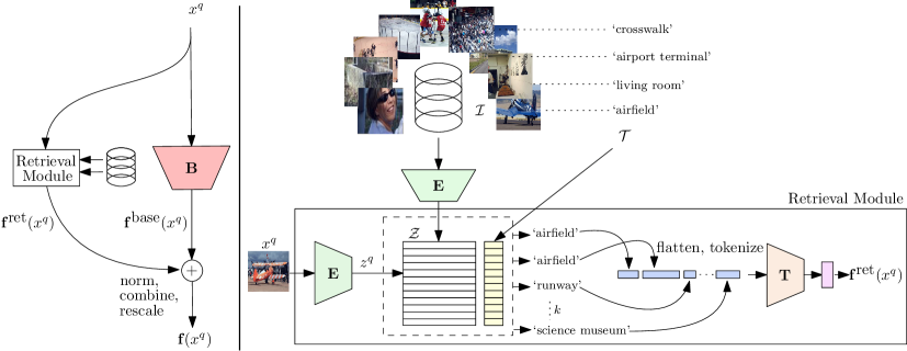
(a) The proposed RAC architecture                                                                         (b) Retrieval module                                                     

Figure 1: (a) RAC overview. RAC consists of a retrieval module that augments a standard encoder $\mathbf{B}(\cdot)$ with explicit external memory. (b) The retrieval module consists of external images $\mathcal{I}$ encoded by a fixed, pretrained image encoder $\mathbf{E}(\cdot)$, and associated text $\mathcal{T}$ queried using an approximate $k$-NN and encoded via a text encoder $\mathbf{T}(\cdot)$. The logits of the retrieval encoder are then combined with those of the base network. In our instantiation, $\mathbf{B}$ and $\mathbf{E}$ are ViT’s, and $\mathbf{T}$ is a BERT-like text encoder.

An alternative approach focuses on ensembling models. Instead of disregarding knowledge of the test distribution, recent work [18, 60, 53] use ensembling models to induce invariance to the test distribution. This is typically done by training separate models under different losses or re-sampling techniques, and combining them at test time.

We introduce a third approach, Retrieval Augmented Classification (RAC), motivated by the desire to explicitly store tail knowledge, as a retrieval-based augmentation to standard classification pipelines.

RAC’s retrieval module is multi-modal, making use of image representations as retrieval keys, and returning encoded textual information associated with each image. We place no limitation on the nature of this text; it may be the labels from a supervised training set, descriptions, captions etc. In the simplest case, the images in the index, and associated text, can be the images and labels from the dataset of interest alone.

RAC jointly trains a standard base encoder, and a separate retrieval branch. We demonstrate empirically that the retrieval branch learns, without explicit prompting, to focus on tail classes. This frees the base encoder from modelling these sparse classes, as they are already effectively represented by the non-parametric memory of the retrieval module. This in turn allows the base encoder to achieve a higher level of performance on the head classes.

RAC achieves state-of-the-art performance on common Long-Tail classification benchmarks, even out-performing approaches such as LACE [38] that are provably consistent with regard to the class-balanced error, and Bayes-optimal under Gaussian class priors. A major benefit of RAC is its ability to use large, pretrained models for inference (for index and retrieval encoding), leveraging their rich representations to improve the classification performance of a base learner. This broadens the applicability of such models due to the large cost of fine-tuning.

Our contributions are summarised as follows:

1. The first demonstration of effective external memory within long-tail visual recognition setting.

2. A novel method for Long-Tail Classification that significantly improves on the current state-of-the-art.

3. Insight into the proposed method, with the reimplementation of strong baselines that also exceed current state-of-the-art.

2 Related Work

Resampling and Logit Adjustment Over-sampling sparse classes [3, 20] is one of the oldest approaches to addressing distribution bias, but one that is still in common use. Under-sampling common classes [13], applying additional data-augmentation to sparse classes in pixel, or feature space [5, 33], or sampling uniformly from pre-computed clusters [23], have also been suggested. Hong et al. [22] propose a distribution aware weight regularizer that is applied more heavily to head classes than tail classes, in a similar vein to weight normalization. However, empirically, the resulting model (LADE) only produces marginal gains over straight-forward balanced softmax. Recent work [38] has unified many empirically successfully approaches under a Fisher-consistent scorer for the balanced error, and additionally shown that weight normalization fails when used with the ADAM optimizer. Zhang et al. [55] adopt a two stage approach, and propose a class-specific learnable (from the samples) reweighting (via a single layer NN) of the frozen pretrained logits based on a generalized formulation of the class-balanced softmax. They show that transforming the classification head, as opposed to re-training it, performs better. PaCo [7], the current state-of-the-art for long-tail classification, combines learnable logit adjustment with contrastive learning[40]. Despite their simplicity, adjusted logit methods (LACE, LDAM, LADE) remain strong solutions to the long tail problem, typically achieving within $1$-$2$% top-1 accuracy of state-of-the-art ensemble approaches (see Table 1, Table 2).

Ensemble Methods In proposing TADE [57], Zhang et al. explicitly train three heads with standard, balanced, and inversely weighted softmax losses, linearly combining their predictions at test time, weighted by a measure of confidence derived from each head’s stability under data-augmentation. Wang et al. [52] in contrast combine multiple independently trained classification heads that are pushed to be decorrelated in their predictions via a (class balanced) KL loss, with a small routing network that improves computational efficiency during inference.

External Memory One of the first models to successfully combine deep networks with external memory was the Neural Turing Machine [16]. The purpose of that model was symbolic manipulation, however, which renders its architecture quite different to that of RAC. Gong et al. [15] proposed a similar retrieval-module architecture for anomaly detection, but without RAC’s corresponding base module. Recently, in the NLP domain, several works have proposed the augmentation of large language models with a non-parametric memory to allow explicit access to external data [31, 19]. While such approaches make use of differential retrievers, which introduces the problem of lookup/representation drift, they are still closely related to RAC. $k$-NN Language Models (LMs) [28] are most similar to our work, which directly interpolate a retrieval distribution with the next token distribution produced by a base LM, resulting in reduced combined model perplexity.

Latent retrieval has been applied to textual open-domain QA[30, 26]. The central difference is such approaches return information that is most similar to the retrieval key, whereas RAC returns information (text) attached to retrieved samples. An approach similar to that of RAC has been applied to knowledge-intensive QA [51], where a ‘fact memory’ consisting of triples from a symbolic Knowledge Base (KB) is directly encoded and queried using the final representation of a language model as keys. In computer vision, non-parametric retrieval has been used to assist in addressing the fine-grained retrieval problem, such as in enforcing instance-level retrieval loss in [48]. The Open-world Long-tail model proposed in [34] also makes use of a retrieval module, but primarily as a mechanism to distinguish between seen, and unseen samples in the ‘open world’ setting, not to boost performance on seen classes as we do.

3 Method

3.1 Preliminaries

In long-tailed visual recognition, the model has access to a set of $N$ training samples $\mathcal{S}=\{({\mathbf{x}}_{n},y_{n})\}^{N}_{n=1}$, where ${\mathbf{x}}_{n}\in\mathcal{X}\subset\mathbb{R}^{D}$ and labels $\mathcal{Y}=\{1,2,..,L\}$. Training class frequencies are defined as $N_{y}=\sum_{(x_{n},y_{n})\in\mathcal{S}}\mathds{1}_{y_{n}=y}$ and the test-class distribution is assumed to be sampled from a uniform distribution over $\mathcal{Y}$, but is not explicitly provided during training. The goal is thus to minimize the balanced error, of a scorer ${\mathbf{f}}:\mathcal{X}\rightarrow\mathbb{R}^{L}$, defined as;

$${\rm BE}({\mathbf{x}},{\mathbf{f}}(\cdot))=\sum_{y\in\mathcal{Y}}{\mathbf{P}}_{{\mathbf{x}}|y}\left(y\notin\operatorname*{arg\,max}_{y^{\prime}\in\mathcal{Y}}{\mathbf{f}}_{y^{\prime}}({\mathbf{x}})\right)$$ (1)

where ${\mathbf{f}}_{y}(x)$ is the logit produced for true label $y$ for sample ${\mathbf{x}}$. Traditionally this is done by minimizing a proxy loss, the Balanced Softmax Cross Entropy (BalCE):

$$\ell_{\text{BalCE}}({\mathbf{x}},y,{\mathbf{f}}_{y}(\cdot))=-\frac{1}{N_{y}}\log\frac{e^{{\mathbf{f}}_{y}({\mathbf{x}})}}{\sum_{y^{\prime}\in\mathcal{Y}}e^{{\mathbf{f}}_{y^{\prime}}({\mathbf{x}})}}.$$ (2)

This is a form of re-weighting, where the contribution of each label’s individual loss is scaled by an approximation of ${\mathbf{P}}(y)$, which for $\ell_{\text{BalCE}}$, is the inverse class frequency. BalCE remains a strong baseline in this domain (see Sec. 4.3).

3.2 LACE Loss

An alternative to re-weighting is to adjust the logits themselves, however the two can be done in conjunction, resulting in the general form of the re-weighted (via $\alpha_{y}$) and adjusted (via $\Delta y$) softmax cross entropy loss;

$$\ell({\mathbf{x}},y,{\mathbf{f}}_{y}(\cdot))=-\alpha_{y}\log\frac{e^{{\mathbf{f}}_{y}({\mathbf{x}})+\tau\cdot\Delta y}}{\sum_{y^{\prime}\in\mathcal{Y}}e^{{\mathbf{f}}_{y^{\prime}}({\mathbf{x}})+\tau\cdot\Delta y^{\prime}}}$$ (3)

where $\tau$ is a constant temperature scaling parameter. Several recent works focusing on long-tail learning exploit special cases of this loss. If $\alpha_{y}=1$ and, Logit Adjusted Cross-Entropy (LACE) [38], can be recovered with $\Delta_{y}=\log\left({N_{y}}/N\right)$ and LDAM [1] with $\alpha_{y}=\nicefrac{{1}}{{N_{y}}}$ and

$$\Delta y=\begin{cases}N_{y}^{-1/4}&\text{if}\quad y^{\prime}=y,\\ 0&\text{otherwise.}\end{cases}$$ (4)

Both are Fisher-consistent with respect to the balanced loss. The optimal $\tau$ can be found with a holdout set, or set to 1 if the logits are calibrated [17]. In our experiments, this calibration is achieved through label smoothing [39], which has been shown to implicitly calibrate neural networks[47]. This property is important in the design of RAC as we use LACE as the base loss and do not apply manual temperature adjustment, setting $\tau=1$, unless otherwise specified.

3.3 Retrieval Augmented Classification

The overall idea of RAC is very simple—Split the scorer into two branches (see Fig. 1), where one branch (retrieval) exhibits implicit invariance to class frequency. The two branches are trained under a common LACE loss, with their individual logits combined with a norm, addition and re-scale operation to ensure that one does not override the other during training.

The base branch encoder $\mathbf{B}(\cdot)$ can be any choice of a standard backbone network. In our experiments, we primarily use the ViT-B-16 variant of Visual Image Transformer [12], transforming the final token embedding via a standard linear layer. The retrieval module (see Sec. 3.4) takes a raw image and performs a latent-space lookup on an index of precomputed embeddings, returning the text attached to the top $k$ most similar images to the image currently being considered, ${\mathbf{x}}^{q}$. This text is then fed through a text encoder and transformed by another linear layer into logits ${\mathbf{f}}^{\text{ret}}({\mathbf{x}}^{q})$.

We make use of the pretrained BERT-like text encoder (63M parameters, 12-layer 512-wide model with 8 attention heads) from CLIP [44], which we choose due to the broad (400M) range of images, alt-text pairs used during pretraining, and the compatibility with other language models due to the preservation of masked self attention in the architecture. In our experiments, the choice of text encoder is not critical as the textual information being retrieved (labels) is not highly complex, and off-the-shelf word embeddings, and even random encodings still perform reasonably well (see Fig. 4). This choice does increase training time due to the larger parameter count (see Table 5), but allows RAC to scale to more complex retrieved text.

To combine base and retrieval branches, we normalize each branch’s outputs to the unit norm and add them together. To ensure training dynamics are not altered (via lower logit magnitudes) in comparison to the baselines we rescale the combined logits by a constant factor (dependent on $L$ due to final layer Xavier initialization [14] also being dependent on $L$).

$${\mathbf{f}}({\mathbf{x}})=\frac{L}{2}\left(\frac{{\mathbf{f}}^{\text{ret}}({\mathbf{x}})}{||{\mathbf{f}}^{\text{ret}}({\mathbf{x}})||_{2}}+\frac{{\mathbf{f}}^{\text{base}}({\mathbf{x}})}{||{\mathbf{f}}^{\text{base}}({\mathbf{x}})||_{2}}\right),$$ (5)

where ${\mathbf{f}}^{\text{base}}({\mathbf{x}})$ represents the logits produced by the image encoder backbone, and ${\mathbf{f}}^{\text{ret}}({\mathbf{x}})$ is the output of the retrieval module. This straightforward setup has the benefit of being able to treat the branch outputs as individual logits, increasing the interpretability of RAC, and allowing us to precisely evaluate the per-class accuracy of each branch (see Fig. 2). While there are many ways to combine the branches such as confidence or distance based weightings, attention mechanisms etc., we found this approach sufficient, with the weighting of each branch done implicitly by the learned sharpness of the logits.

3.4 Retrieval Module

Figure 2: Per-class top-1 accuracy on Places365-LT from each branch’s output. Without prompting, the retrieval module learns to focus on tail classes. The $20$ sample moving average over classes (solid line) is shown for clarity.

The retrieval module consists of a frozen pretrained image encoder $\mathbf{E}(\cdot)$, a pre-existing set of external images $\mathcal{I}=\{{\mathbf{i}}_{j}\}_{j=1}^{J}$, with associated text $\mathcal{T}=\{{\mathbf{t}}_{j}\}_{j=1}^{J}$, which may be labels, descriptions, captions etc. Unless otherwise specified $\mathbf{E}(\cdot)$ is a ViT-B-16, pretrained on ImageNet following [45]. Prior to training RAC, the retrieval module is initialized by producing image keys $\mathcal{Z}=\{{\mathbf{z}}_{j}\}$ such that ${\mathbf{z}}_{j}=\mathbf{E}({\mathbf{i}}_{j})\;\forall j$, and storing the resultant representations in a fast approximate $k$-NN index.

During training, we produce features ${\mathbf{z}}^{q}=\mathbf{E}({\mathbf{x}}^{q})$ for each image ${\mathbf{x}}^{q}$ in the training batch. The $k$-NN is queried for each ${\mathbf{z}}^{q}$ and returns a list of indices of the $k$ closest keys in $\mathcal{Z}$, where cosine similarity is the distance metric. The text element in $\mathcal{T}$ is recovered for every such index, generating $k$ text elements for each query. These text elements are then encoded by a text encoder $\mathbf{T}(\cdot)$ which produces the retrieval branch’s (fixed length) logits, ${\mathbf{f}}^{\text{ret}}({\mathbf{x}}^{q})$.

Text strings are truncated after 76 tokens, and the resultant batches are zero-padded. This approach allows for a single text-encoder call per batch, as opposed to $k$ which would be required if each text snippet was encoded separately, and would result in a significant slowdown. The use of a large-scale transformer ensures that RAC can scale to longer text snippets if the external information is expanded to contain additional sources beyond simply labels.

A key feature of the retrieval module is its ability to include otherwise unconnected data-sources simply via their labels. In this way, we can dynamically add or remove datasets from $\mathcal{\mathcal{I}}$, and if new examples are similar (from the point of view of the encoder), they can directly impact classification accuracy, providing an alternative to fine-tuning in order to incorporate new information.

For fast querying of the index, we make use of the FAISS implementation [24] of the Hierarchical Navigable Small World (HNSW) approximate $k$-NN lookup [37]. We construct the index with default settings aside from the hyperparameter $M=32$, which sets the number of bidirectional links per node and increases the complexity of the index, but allows for higher recall. During training, we drop the first result, as when training data is included in the index, the first result is often the original image, which causes the text encoder to place undue weight on the first retrieved label when creating predictions.

Method	Many	Med	Few	All
Input: $224\times 224$
OLTR [34] $\dagger$	59	64.1	64.9	63.9
Decouple-LWS [25] $\dagger$	-	-	-	65.9
LADE [22] $\dagger$	-	-	-	69.3
Grafit [48]	-	-	-	69.9
ALA [58]	71.3	70.8	70.4	70.7
RIDE [52] (2 experts)	70.2	71.3	71.7	71.4
LACE [38]	-	-	-	71.9
RIDE [52] (4 experts)	70.9	72.4	73.1	72.6
TADE [57]	74.4	72.5	73.1	72.9
DisAlign [55]	-	-	-	74.1
PaCo [7]	75.0	75.5	74.7	75.2
RAC (ours)	75.92	80.47	81.07	80.24
Input: $384\times 384$
Grafit	-	-	-	81.2
RAC (ours)	82.91	85.71	86.06	85.56

Table 1: Historical performance on iNat, ^†Results reproduced from [58].

Method	Many	Med	Few	All
Focal Loss [32] $\dagger$	41.1	34.8	22.4	34.6
Range Loss [56] $\dagger$	41.1	35.4	23.2	35.1
OLTR [34] $\dagger$	44.7	37	25.3	35.9
Decouple-LWS [25] $\dagger$	40.6	39.1	28.6	37.6
LADE [22] $\dagger$	42.8	39	31.2	38.8
DisAlign [55]	40.4	42.4	30.1	39.3
ALA [58]	43.9	40.1	32.9	40.1
TADE [57]	43.1	42.4	33.2	40.9
PaCo [7]	36.1	47.9	35.3	41.2
RAC (ours)	48.69	48.31	41.76	47.17

Table 2: Historical performance on Places365-LT. ^†Results reproduced from [58].

4 Experiments

Method	$\mathbf{B}$	Many	Med	Few	All
Places365-LT
CE	RN50	-	-	-	32.14
BalCE	RN50	-	-	-	38.31
CE	ViT-B-16	50.81	33.83	19.51	37.16
BalCE	ViT-B-16	49.03	45.72	29.05	43.67
Retrieval	-	43.50	41.99	26.83	39.58
Base	ViT-B-16	44.57	45.06	40.77	44.05
RAC	ViT-B-16	48.69	48.31	41.76	47.17
iNaturalist 2018
CE	RN50	-	-	-	61.7
BalCE	RN50	-	-	-	69.8
CE	ViT-B-16	81.53	76.62	69.82	74.44
BalCE	ViT-B-16	72.39	76.06	73.05	74.49
Retrieval	-	50.10	52.77	52.45	52.37
Base	ViT-B-16	74.41	78.95	78.55	78.32
RAC	ViT-B-16	75.92	80.48	81.07	80.24

Table 3: Comparison of top-1 accuracy against baselines under a common training scheme. Column $\mathbf{B}$ indicates the architecture of the base branch.

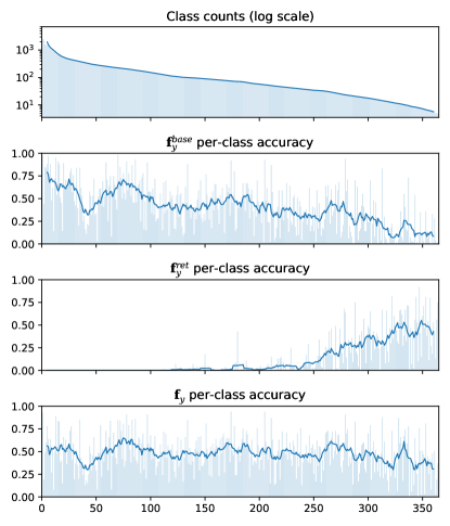
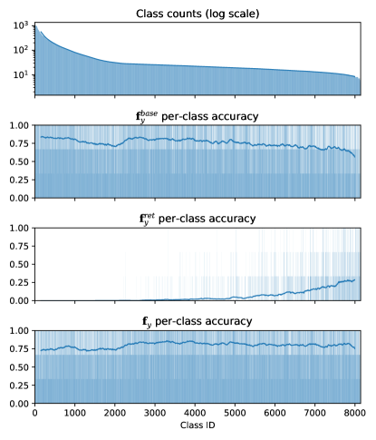
We establish RAC’s high level of performance on common benchmark datasets iNaturalist2018 (Table 1) and Places365-LT (Table 2) with no additional external information aside from the datasets used to pretrain the individual encoders. Note that these tables report results from the literature which were obtained under varying architectures and training schemes. We ablate the benefit of RAC’s improved training pipeline in Table 3 where we reimplement class-balanced softmax Cross Entropy (BalCE) and LACE [38] as baselines. We consider ‘Base’ trained under the LACE loss [38] as our primary baseline, due to LACE’s strong theoretical grounding, provable consistency, and high level of previously reported empirical performance. We report overall accuracy as well as per-class accuracy bucketed into the few ($<20$), medium ($\leq 100$) and many ($>100$) shot categories. The full per-class distribution curve is also shown in Fig. 2. We then focus specifically on the design choices of the retrieval module and how the choice of data for the index affects RAC in Sec. 4.7.

In all experiments, unless otherwise indicated, $\mathbf{E}$ is a ViT-B-16 encoder, with the weights from [12]. The weights are obtained from pretraining on ImageNet21k (IM21k), a larger (11M samples) variant of the original 1.2M images ImageNet [10] dataset, with more granular classes. We make use of IM21k to expand the index in some experiments, and use the variant introduced in [29].

4.1 Places365-LT

Places365-LT is a synthetic long-tail variant of Places-2 [61] introduced in [34]. It consists of $365$ high-level scene classes such as ‘airport’, ‘basement’, etc. across $62.5$K samples at $256\times 256$ resolution. The minimum number of samples per class is $5$, with a training set that, while balanced, is not perfectly uniform. The dataset contains a significant amount of label noise, which makes it appealing, as logit adjustment methods typically assume fully separable classes in their theoretical motivation.

We observe that with no explicit prompting, the retrieval network learns to highly skew its accuracy towards the few-shot classes (Fig. 1), confirming our hypothesis that it will be beneficial in this case. Note that there is no explicit signal pushing the retrieval network to learn infrequent classes over common ones, or for the supervised network to prefer common classes, as both are trained under the common LACE loss. Interestingly, RAC’s learned strategy is similar to the hard-coded ensembling utilized in TADE [57], which is the previous state-of-the-art.

4.2 iNaturalist-2018

iNaturalist-2018 (iNat) [49] consists of $437$K images and $6$ levels of label granularity (kingdom, genus etc.). Following other work, we consider only the most granular labels (species), which constitutes $8142$ unique classes with a naturally occurring class imbalance. In many cases the labels are very fine-grained, making it a challenging dataset even without the long-tailed property. The test set is perfectly balanced, with $3$ samples per class.

In addition to the $224\times 224$ resolution commonly studied, we report the results with $384\times 384$ images, which was used in GRAFIT [48] and is currently state-of-the-art for this task. We found the use of $16\times 16$ patch size to be of major importance on iNat, boosting retrieval accuracy by $21.6\%$ (see Table 4), likely due to the fine-grained nature of the dataset.

4.3 Ablation

Encoder	Many	Med	Few	All	CT(m:s)
Places365-LT
RN50	31.73	16.28	8.65	20.34	0:46
RN152d	33.52	17.71	10.03	21.89	2:07
ViT-B-32	38.34	24.82	15.83	27.92	0:20
ViT-B-32∗	39.95	26.12	16.87	29.28	0:49
ViT-B-16	39.97	26.74	18.65	29.91	0:53
ViT-B-16∗	40.79	27.23	19.25	30.55	3:15
iNaturalist 2018
RN50	26.8	20.8	21.15	21.56	5:14
RN152d	38.95	29.56	28.45	30.09	17:50
ViT-B-32	48.14	43.69	44.1	44.31	2:35
ViT-B-16	59.38	53.92	52.42	53.89	4:19
ViT-B-16∗	66.15	61.54	60.92	61.77	22:14

Table 4: Analysis of standard retrieval performance and Construction Time (CT) which includes both image encoding and HNSW indexing. ${}^{*}384\times 384$ resolution variants.

We baseline RAC’s performance against class-balanced softmax cross entropy (BalCE) and with the retrieval branch removed (Base only variant) under a common training setup in Table 3. We also include final accuracies for ResNet models for comparison. RAC consistently increases all-class top-1 accuracy by $8.04\%$ on Places365-LT and $7.72\%$ on iNat over BalCE, and by $25.48\%$ over standard cross entropy on Places365-LT. These improvements are most pronounced on the tail classes where RAC improves over BalCE by $30.42\%$ on Places365-LT and $10.98\%$ on iNat.

One question is how RAC is able to so outperform methods that are provably consistent, such as LACE [38]. We hypothesize that, in addition to the non-convexity introduced by using Neural Networks as the scorer, this is due to the fact that sample frequency alone does not indicate classification ‘difficulty’ from the perspective of a balanced learner [59]. Instead, a small number of samples may still define a sufficiently clear decision boundary if the volume of semantic space covered by that class is small and distinct [8], and hence in a truly balanced model, both inter- and intra-class distributions must be considered. Accounting for the intra-class distribution being difficult, however, given no prior on this quantity is typically provided, aside from the labels themselves. Instead, the majority of prior work has either ignored this factor, or assumed the class distributions to be Gaussian. In our formulation, these “easy” classes get picked up by the retrieval model, leaving the base branch to focus on examples that are difficult, where the difficulty is a combination of presentation frequency and class complexity. Previous methods have attempted this by correlating stability under augmentation with confidence [57], however, this correlation is weak.

Figure 3: Effect of the number of retrieved text snippets, $k$, on Places365-LT top-1 accuracy for the retrieval only branch, querying an index containing only the Places365-LT training set. Higher $k$ consistently improves performance until the cutoff induced by the text encoding truncation ($76$ tokens), however it does come at the cost of (linearly) higher training time. We choose $k=30$ in our experiments. $x$-axis is log-scaled.

4.4 Retrieval

Quantifying retrieval accuracy is important because if standard retrieval performance is significantly lower than that of a balanced supervised learner such as the LACE baseline, it is unlikely to be beneficial. In Table 4 we perform standard retrieval with ImageNet pretrained encoders on both datasets, encoding the training set and then querying it with encoded test images, returning the label of the closest image in the training set as the prediction. All comparisons are done on exact match indexes with the $\ell_{2}$ distance, no data augmentation and consistent crop, interpolation and normalization constants. $z_{q}$ has length $2048$ for the ResNet models, and $768$ for ViTs. Despite being trained on the same data, we show that ViTs significantly outperform ResNets, and are hence critical to RAC’s performance.

4.5 Importance of the Text Encoder

Figure 4: Effect of the choice of text encoder on performance. The overall impact is minor, however the CLIP LM significantly boosts few-shot performance on Places365-LT, where labels are natural language terms.

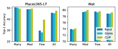
RAC makes use of a large BERT-like text encoder to learn a mapping from retrieved labels to class logits. Here we quantify the importance of this model relative to two alternatives: (i) Bag-of-words (BoW) GLoVe[42] embeddings, and (ii) BoW cached random embeddings.

Both are of dimension $300$ vs.  $512$ for the CLIP encoder. The random embeddings are sampled from a uniform distribution over the interval $[0,1)$ and cached for each word in the input string. That is, the embeddings for individual words are consistent, but have no inherent semantics.

We observe that a higher capacity $\mathbf{T}$ does improve performance, particularly on the Places365-LT few-shot classes, but that overall this benefit is minor. This is likely due to the input to the encoder not being overly complex, and more detailed information such as captions were returned, this effect may be more pronounced.

Figure 5: Effect of index content on performance ($k=30$) on the retrieval branch only, trained under the LACE loss on Places365-LT. Here, the index contains no Places365-LT data, only variants of the ImageNet21k dataset.

4.6 Effect of $k$

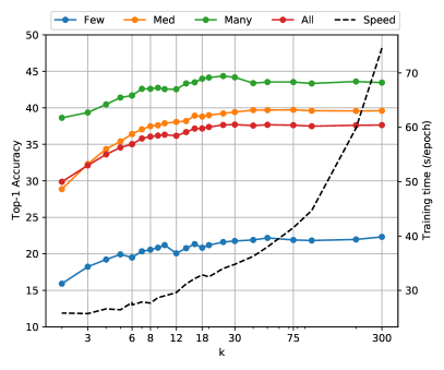
Given that our choice of $k$ in approximate $k$-NN search is larger than the minimum number of samples present per-class for both Places365-LT and iNat, we question whether the additional returned samples, which cannot be the correct class (in the few-shot case), degrade retrieval performance. To study this, we experimented on only the retrieval branch, with no base encoder, and utilized an index that contained the training set only. As can be seen in Fig 3, increasing $k$ consistently increases accuracy, indicating the text encoder $\mathbf{T}(\cdot)$ is able to learn to disregard the common classes. Note the few-shot performance is low here, as the retrieval branch is still trained under the LACE loss, and hence pushed towards balanced performance across all classes. It is thus not free (via the base branch) to focus on the tail classes. This indicates that newer transformer architectures, that facilitate longer sequence length, may be beneficial when applied to RAC, especially when the associated text snippets themselves are longer.

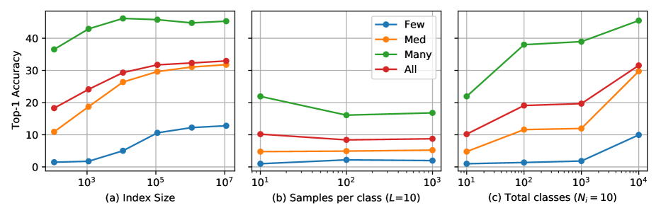
4.7 Impact of Index Content

To quantify how index content affects RAC, we carried out three experiments in which we trained only the retrieval module on the Places365-LT dataset, with variants of the ImageNet21k dataset used for the index. Training was done with the same final LACE loss as complete RAC, with a ViT-B-16 as $\mathbf{E}$. Specifically, we alter:

1. the index size via directly sub-sampling from the full ImageNet21k dataset.

2. the number of training examples per-class while keeping the number of classes constant.

3. the number of classes while keeping the number of sample per class constant.

Results are shown in Fig. 5. While naively increasing index size does increase performance, this effect diminishes as more samples are added. This is likely caused by the information content of the labels passed to $\mathbf{T}$ not increasing—as once most labels are present $\mathbf{E}$ is more likely to find a similar image, however from the perspective of $\mathbf{T}$, which is not distance or image aware, the information is the same. This is supported by sub-figures (b) and (c), in which the total amount of samples in the index is increased consistently between both plots, but adding samples by via new labels has a disproportionately larger effect than adding new samples with the number of labels constant. This is promising in that it indicates increasing label granularity, through the use of image captions or associated text, is likely to increase RAC’s performance even further.

4.8 Runtime Consideration

Nearest neighbour searches can be computationally infeasible for large datasets. We show here, however, that a lookup over a sample index of size $>$10M can be performed for each training sample with negligible overhead, although the additional label encoding (and subsequent backprop), does increase the training time by a factor of $1.5-2\times$. We report the precise run-times of models with and without retrieval augmentation on Places365-LT in Table 5. Given that the index is static, the number of iterations per second is constant throughout training. All training is carried out on a single node, containing $8\times$ A$100$ GPUs ($32$GB Mem).

Moving a tensor from the GPU to CPU, querying the index, then moving the resultant tensor back to GPU maybe expected to slowdown training. However, we find that the impact is minor with the majority of overhead coming from the additional text encoder (the random encoder, ‘Rand.’, contains no additional parameters). To facilitate multi-node training, RAC keeps separate, complete copies of each index in memory for each node, ensuring querying the index is never the bottleneck, which we found to be essential. While it is possible to do the search entirely on GPU, due to the low overhead we do not do this, instead using the free GPU memory to facilitate a large batch size. Due to the use of HNSW, index query time is logarithmic with respect to the index size, and a standard exhaustive search is prohibitively slow.

Index Data	Size	Text Enc.	Speed (s/epoch)
None	None	None	$23.6$
Places	$184$K	Rand.	$28.3$
Places	$184$K	CLIP	$44.3$
Places, IM21k	$11.2$M	CLIP	$47.0$

Table 5: Effect of additional text encoder, and lookup on training wall-time for RAC ($k=50$) on Places365-LT. Top row indicates the use of the base encoder only. The majority of added overhead comes from use of the text encoder, rather than the lookup itself.

5 Limitations

While RAC demonstrates robust performance for both naturally occurring (iNat) and constructed (Places365-LT) long-tailed class distributions, the analysis could be further expanded to include additional long-tailed datasets. The performance of RAC on balanced datasets is also of interest and not explored. Finally, while RAC clearly demonstrates the benefit of an explicit retrieval component, the data being retrieved (labels) is of limited value and imposes a cap on RACs performance—a natural extension is to query for whole paragraphs or captions. However, the 76 token limit imposed by the CLIP text encoder prevents this, and would need to be increased. We leave this for future work.

6 Conclusion

We have introduced RAC, a generic approach to augmenting standard classification pipelines with an explicit retrieval module. RAC’s retrieval module, without prompting, achieves a high level of accuracy on tail classes, freeing up the base encoder to focus on common classes. RAC improves upon the state-of-the-art results on the iNat and Places365-LT benchmarks by a large margin for the task of long-tail image classification. We hope that RAC represents a step towards more effectively making use of external memory within common computer vision architectures, and we predict its use for other vision tasks, particularly, such as one/few shot learning, and continual learning without catastrophic forgetting.

Appendix

We provide more information here.

Appendix A Additional Experiments

A.1 Re-weighting and Temperature Scaling

Places365-LT
Re-weighting	Many	Med	Few	All
None	49.72	49.34	40.46	47.75
Inverse sqrt.	47.12	49.58	47.65	48.32
Inverse log	44.88	51.35	47.54	48.29
iNat
None	75.92	80.48	81.07	80.24
Inverse sqrt.	71.13	80.02	81.19	79.56
Inverse log	67.17	80.04	81.67	79.35

Table S1: Effect of common re-weighting schemes when combined with logit adjustment for RAC’s top-level loss.

As a top level loss for RAC, we make use of unscaled logit adjustment exclusively, with no reweighting (i.e. $\alpha_{y}=1\quad\forall y\in\mathcal{Y}$) and no temperature scaling ($\tau=1$) in Eq. 3. This loss is theoretically well-grounded [38], and is appealing due to its simplicity. Nevertheless, other works have noted that the combination of logit adjustment with re-weighting often leads to higher empirical performance [1]. While optimizing the top-level loss is not the focus of RAC, we include here a comparison of RAC performance under various re-weighting schemes when combined with logit adjustment for completeness. Specifically, we consider inverse log

$$\alpha_{y}=\frac{1}{\log{N_{y}}}$$ (6)

and inverse square-root

$$\alpha_{y}=\frac{1}{\sqrt{N_{y}}}$$ (7)

class-frequency based re-weighting of individual sample losses.

We confirm that the same effect is present for RAC on Places365-LT, with overall accuracy increasing with the use of both re-weighting schemes, with improvement most pronounced for tail classes (Table S1). However, this trend does not hold on iNat.

Figure S1: Effect of $\tau$ within the LACE loss on balanced performance on the Places365-LT dataset.

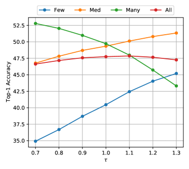
For Places365-LT, we also we perform a sweep across $\tau$, to evaluate if the same effect can be achieved with manual temperature scaling (Fig. S1). Higher $\tau$ does result in slightly higher overall accuracy, however this effect is minor in comparison to re-weighting. This divergence from theory is likely due to the non-separability of many classes in Places365-LT due to the high label noise.

A.2 Index Ablations

Index Size	Index Type	Distance	Test					Train	QT (ms/sample)
			Many	Med	Few	Top-1	Top-5	Top-1
62.5k	Exact	$L_{2}$	39.97	26.74	18.65	29.91	53.81	99.97	1.12
62.5k	Exact	Cosine	39.84	26.51	18.03	29.64	53.31	99.96	1.14
62.5k	HNSW	$L_{2}$	39.89	26.51	18.03	29.66	53.32	99.79	1.06
62.5k	HNSW	Cosine	39.57	26.26	17.68	29.37	52.83	99.79	1.07
11.2M	Exact	$L_{2}$	-	-	-	-	-	-	7.96
11.2M	HNSW	$L_{2}$	-	-	-	-	-	-	3.01

Table S2: Index ablations on Places365-LT. QT indicates Query Time. Large-sample indices are filled with the ImageNet21k dataset.

We examine the effect of the distance metric and index type on RAC’s lookup performance and speed in Table S2. To quantify error induced by an approximate index, we include the lookup accuracy on the index content itself (training set) in addition to the validation accuracy. Query Time (QT) includes encoding samples with a ViT-B-16 model, which is the primarily overhead on small indexes.

We observe that the choice of distance metric ($\ell_{2}$ vs.  cosine) has little effect, as may be expected, give the high dimentionality of the index. Cosine distance does introduce a minor computational overhead due to the need to normalize the embeddings prior to querying. The drop in accuracy due to use of an approximate (HNSW) instead of exact $k$-NN is also minor, but comes with a significant (2$\times$) speedup on large index’s. Construction time is constant across all indexes at $0.02\mu$s per sample, with the exception of large-index HNSW, which requires $0.05\mu$ per sample. In summary, performance differences are minor when querying small indexes, however as the index size grows, the choice of HNSW becomes critical to ensure lookup time does not bottleneck training.

A.3 Per-class Accuracy on iNat

We include the same per-class visualization presented in the main body for Places365-LT (Fig. 2), for iNat. Note that for iNat only 3 samples are present for each class in the validation set, hence the square-wave appearance of the plots (Fig. S2). Nevertheless, the same trend is clearly visible in the sliding window moving average, with the retrieval module performing best on tail classes and the base network largely focusing on the many and mid-frequency classes.

Figure S2: Per-class top-1 accuracy on iNat from each branch’s output. The $300$ sample moving average over classes (solid line) is shown for clarity.

Appendix B Further Details

For Places365-LT we use the training and validation splits during development and report final numbers on the test set, with no validation samples used during final training. For iNaturalist2018, following prior work, we report results on the released validation split, as labels for the test set are not publicly available.

In the main text, we use several common model variants. While the architectures for these models are standard, we specify the high-level design choices in Tables S5 and S4. These choices are consistent across both the $224\times 224$ and $384\times 384$ variants.

	Places365-LT	iNat
Samples (train)	62,500	437,513
Samples (test)	36,500	24,426
Classes	365	8,142
Imbalance Factor	500	996

Table S3: Dataset Details

Hyperparameter	ViT-B-16	ViT-B-32
Patch size	16	32
Depth	12	12
Embedding Dimension	768	768
Attention Heads	12	12
Parameters	85.8M	87.4M

Table S4: ViT model architecture details.

Hyperparameter	RN50	RN152d
Input size	$244\times 224\times 3$	$256\times 256\times 3$
Head	Avg. Pool, FC	Avg. Pool, FC
Convolutions	standard	standard
Stem Convolutions	1 layer, $3\times 3$	3 layer, $3\times 3$
Stem width	32	(128, 128, 128)
Layers	[3, 4, 6, 3]	[3, 8, 36, 3]
Pool size	$7\times 7$	$8\times 8$
Num. features	2048	2048
Parameters	23.5M	58.2M

Table S5: ResNet model architecture details.

All training is carried out on $8\times$ $32$GB A$100$ GPU’s. We largely follow the procedures outlined in [45], with the following alterations. We finetune with AdamW [35] instead of SGD, and make use of low-magnitude RandAugment [6] alone for data augmentation, with no Color-Jitter, Mixup, Cutmix, RandomErase or Augmix applied. Full hyperparameters are shown in Table S7. While we found the use of Mixup and Cutmix does boost performance on standard ViTs trained under a BalCE loss, their use of combined targets requires special treatment to make compatible with the LACE loss, which requires hard targets in order to assign the class adjustment. While one approach may be to apply the ‘merged’ class adjustment, the performance benefit is marginal and hence we simply did not include either approach in RAC’s data augmentation pipeline.

	Places365-LT	iNat
Batch Size	200	50
Learning Rate	5e-5	1e-4
Epochs	30	20

Table S6: Dataset specific training hyperparameters

Hyperparameter	Value
Global normalization means	[0.5, 0.5, 0.5]
Global normalization stds	[0.5, 0.5, 0.5]
Crop (train and test)	0.95
Distributed	DDP 8 GPU’s
LR schedule	cosine
Min LR	1e-7
Warmup LR	1e-7
Warmup epochs	5
Optimizer	adamw
Beta 1	0.9
Beta 2	0.999
Eps.	1e-8
Gradient clipping	$L_{2}$ Norm
Gradient clipping magnitude	1.0
RandAugment magnitude	1
RandAugment layers	3
RandAugment noise std.	0.5
Weight decay	0.02
Label smoothing	0.1
Stochastic depth	0.1
Random erase prob.	0.0
Color jitter	0.0
Random scale	[0.75, 1.33]
Random crop	No
Horizontal flip prob.	0.5
Random rotation	No
Mixed precision level	O2

Table S7: Training hyperparameters for the ViT models

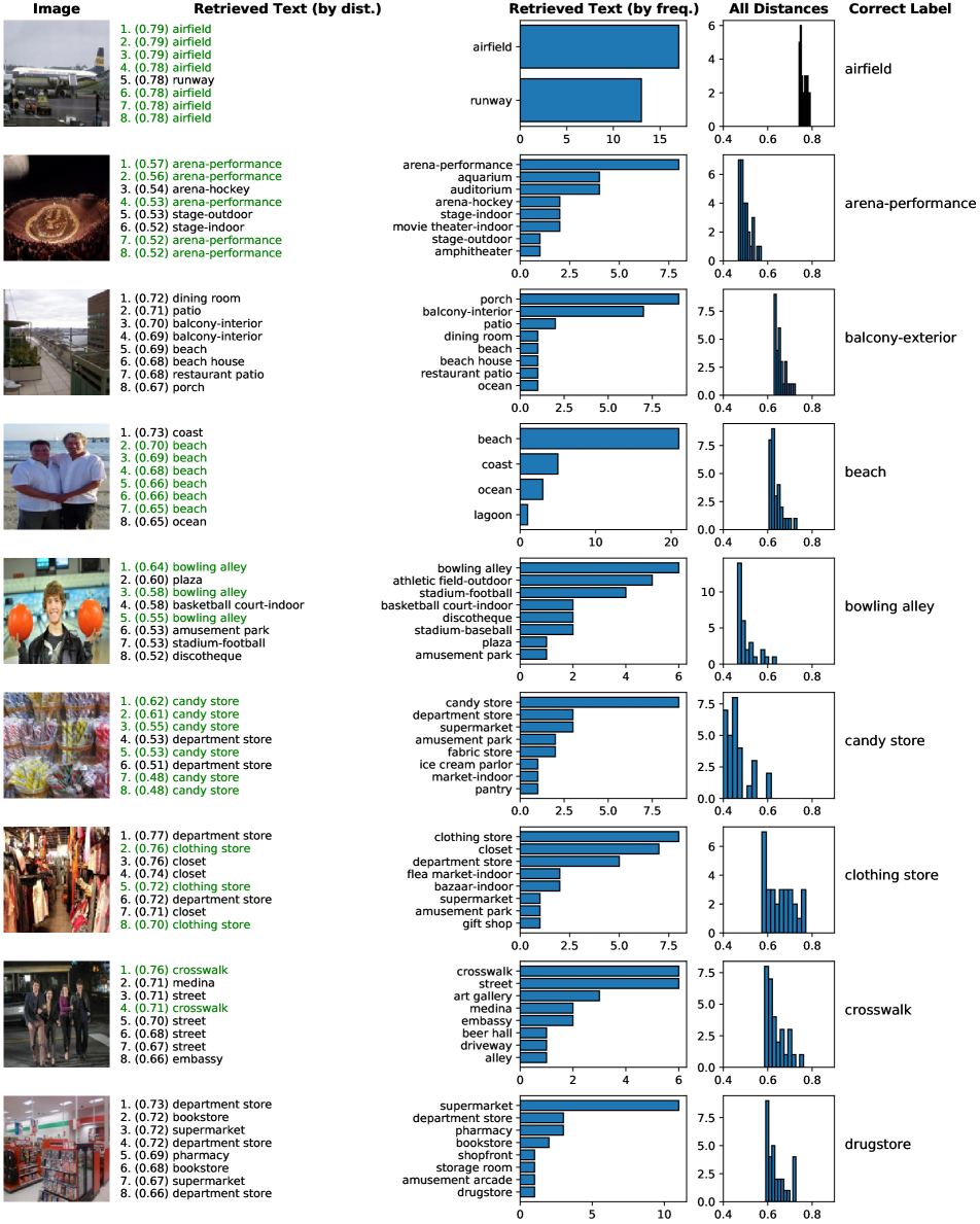
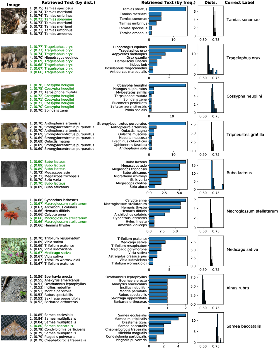
Appendix C Retrieval Branch Visualization

While Table 4 quantifies top-1 performance of the retrieval branch, non-exact match snippets will also effect RAC as they are still likely to be informative. If ‘plane’, ‘runway’, ‘concrete’, ‘sky’, ‘propeller’ etc. are returned for example, it is not difficult for $\mathbf{B}$ to place a high score on ‘airport’. We visualize the returned strings for random samples by distance and frequency in Figs. S3 and S4. For all runs, $k=30$ as in the main work.

Each column displays (from left to right):

1. query image $x_{q}$,

2. retrieved labels sorted by distance (distance shown in brackets, exact matches colored green),

3. retrieved labels and occurrence counts, sorted from most to least frequent,

4. histogram of distances to all returned samples,

5. the correct label.

We restrict the lists of retrieved labels to the top eight for visualization purposes. Note that as the distance metric is cosine, a higher value corresponds to more similar samples.

Figure S3: Retrieval branch visualization for randomly drawn samples from Places365-LT. For detailed explanation see Appendix C.

Figure S4: Retrieval branch visualization for randomly drawn samples from iNaturalist2018. For detailed explanation see Appendix C.

References

- [1] Kaidi Cao, Colin Wei, Adrien Gaidon, Nikos Arechiga, and Tengyu Ma. Learning imbalanced datasets with label-distribution-aware margin loss. arXiv: Comp. Res. Repository, 2019.
- [2] Claire Cardie and Nicholas Howe. Improving minority class prediction using case-specific feature weights. In Proc. Int. Conf. Mach. Learn., 1997.
- [3] Nitesh V Chawla, Kevin W Bowyer, Lawrence O Hall, and W Philip Kegelmeyer. Smote: synthetic minority over-sampling technique. J. Artificial Intelligence Research, 16:321–357, 2002.
- [4] Hila Chefer, Shir Gur, and Lior Wolf. Transformer interpretability beyond attention visualization. In Proc. IEEE Conf. Comp. Vis. Patt. Recogn., pages 782–791, 2021.
- [5] Peng Chu, Xiao Bian, Shaopeng Liu, and Haibin Ling. Feature space augmentation for long-tailed data. In Proc. Eur. Conf. Comp. Vis., pages 694–710, 2020.
- [6] Ekin D. Cubuk, Barret Zoph, Jonathon Shlens, and Quoc V. Le. Randaugment: Practical automated data augmentation with a reduced search space. In Proc. IEEE Conf. Comp. Vis. Patt. Recogn. Workshops, pages 702–703, 2020.
- [7] Jiequan Cui, Zhisheng Zhong, Shu Liu, Bei Yu, and Jiaya Jia. Parametric contrastive learning. In Proc. IEEE Conf. Comp. Vis. Patt. Recogn., pages 715–724, 2021.
- [8] Yin Cui, Menglin Jia, Tsung-Yi Lin, Yang Song, and Serge Belongie. Class-balanced loss based on effective number of samples. In Proc. IEEE Conf. Comp. Vis. Patt. Recogn., pages 9268–9277, 2019.
- [9] Nicola De Cao, Wilker Aziz, and Ivan Titov. Editing factual knowledge in language models. arXiv: Comp. Res. Repository, 2021.
- [10] Jia Deng, Wei Dong, Richard Socher, Li-Jia Li, Kai Li, and Li Fei-Fei. Imagenet: A large-scale hierarchical image database. In Proc. IEEE Conf. Comp. Vis. Patt. Recogn., pages 248–255. Ieee, 2009.
- [11] Zongyong Deng, Hao Liu, Yaoxing Wang, Chenyang Wang, Zekuan Yu, and Xuehong Sun. PML: Progressive margin loss for long-tailed age classification. In Proc. IEEE Conf. Comp. Vis. Patt. Recogn., pages 10503–10512, 2021.
- [12] Alexey Dosovitskiy, Lucas Beyer, Alexander Kolesnikov, Dirk Weissenborn, Xiaohua Zhai, Thomas Unterthiner, Mostafa Dehghani, Matthias Minderer, Georg Heigold, Sylvain Gelly, et al. An image is worth 16x16 words: Transformers for image recognition at scale. arXiv: Comp. Res. Repository, 2020.
- [13] Chris Drumnond. Class imbalance and cost sensitivity: Why undersampling beats oversampling. In ICML-KDD Workshop: Learning from Imbalanced Datasets, volume 3, 2003.
- [14] Xavier Glorot and Yoshua Bengio. Understanding the difficulty of training deep feedforward neural networks. In Proc. Int. Conf. Artificial Intelligence and Statistics, pages 249–256, 2010.
- [15] Dong Gong, Lingqiao Liu, Vuong Le, Budhaditya Saha, Moussa Reda Mansour, Svetha Venkatesh, and Anton van den Hengel. Memorizing normality to detect anomaly: Memory-augmented deep autoencoder for unsupervised anomaly detection. In Proc. IEEE Conf. Comp. Vis. Patt. Recogn., pages 1705–1714, 2019.
- [16] Alex Graves, Greg Wayne, and Ivo Danihelka. Neural turing machines. arXiv: Comp. Res. Repository, 2014.
- [17] Chuan Guo, Geoff Pleiss, Yu Sun, and Kilian Q. Weinberger. On calibration of modern neural networks. In Proc. Int. Conf. Mach. Learn., pages 1321–1330, 2017.
- [18] Hao Guo and Song Wang. Long-tailed multi-label visual recognition by collaborative training on uniform and re-balanced samplings. In Proc. IEEE Conf. Comp. Vis. Patt. Recogn., pages 15089–15098, 2021.
- [19] Kelvin Guu, Kenton Lee, Zora Tung, Panupong Pasupat, and Ming-Wei Chang. Realm: Retrieval-augmented language model pre-training. arXiv: Comp. Res. Repository, 2020.
- [20] Hui Han, Wen-Yuan Wang, and Bing-Huan Mao. Borderline-SMOTE: A new over-sampling method in imbalanced data sets learning. In Proc. Int. Conf. Intelligent Computing, pages 878–887, 2005.
- [21] Haibo He and Edwardo A. Garcia. Learning from imbalanced data. IEEE Trans. Knowledge & Data Engineering, 21(9):1263–1284, 2009.
- [22] Youngkyu Hong, Seungju Han, Kwanghee Choi, Seokjun Seo, Beomsu Kim, and Buru Chang. Disentangling label distribution for long-tailed visual recognition. In Proc. IEEE Conf. Comp. Vis. Patt. Recogn., pages 6626–6636, June 2021.
- [23] Chen Huang, Yining Li, Chen Change Loy, and Xiaoou Tang. Learning deep representation for imbalanced classification. In Proc. IEEE Conf. Comp. Vis. Patt. Recogn., pages 5375–5384, 2016.
- [24] Jeff Johnson, Matthijs Douze, and Hervé Jégou. Billion-scale similarity search with GPUs. arXiv: Comp. Res. Repository, 2017.
- [25] Bingyi Kang, Saining Xie, Marcus Rohrbach, Zhicheng Yan, Albert Gordo, Jiashi Feng, and Yannis Kalantidis. Decoupling representation and classifier for long-tailed recognition. arXiv: Comp. Res. Repository, 2019.
- [26] Vladimir Karpukhin, Barlas Oğuz, Sewon Min, Patrick Lewis, Ledell Wu, Sergey Edunov, Danqi Chen, and Wen-tau Yih. Dense passage retrieval for open-domain question answering. arXiv: Comp. Res. Repository, 2020.
- [27] Salman Khan, Muzammal Naseer, Munawar Hayat, Syed Waqas Zamir, Fahad Shahbaz Khan, and Mubarak Shah. Transformers in vision: A survey. arXiv: Comp. Res. Repository, 2021.
- [28] Urvashi Khandelwal, Omer Levy, Dan Jurafsky, Luke Zettlemoyer, and Mike Lewis. Generalization through memorization: Nearest neighbor language models. In Proc. Int. Conf. Learn. Representations, 2020.
- [29] Alexander Kolesnikov, Lucas Beyer, Xiaohua Zhai, Joan Puigcerver, Jessica Yung, Sylvain Gelly, and Neil Houlsby. Big transfer (bit): General visual representation learning. In Proc. Eur. Conf. Comp. Vis., pages 491–507. Springer, 2020.
- [30] Kenton Lee, Ming-Wei Chang, and Kristina Toutanova. Latent retrieval for weakly supervised open domain question answering. arXiv: Comp. Res. Repository, 2019.
- [31] Patrick Lewis, Ethan Perez, Aleksandra Piktus, Fabio Petroni, Vladimir Karpukhin, Naman Goyal, Heinrich Küttler, Mike Lewis, Wen-tau Yih, Tim Rocktäschel, et al. Retrieval-augmented generation for knowledge-intensive nlp tasks. arXiv: Comp. Res. Repository, 2020.
- [32] Tsung-Yi Lin, Priya Goyal, Ross Girshick, Kaiming He, and Piotr Dollár. Focal loss for dense object detection. In Proc. IEEE Int. Conf. Comp. Vis., pages 2980–2988, 2017.
- [33] Jialun Liu, Yifan Sun, Chuchu Han, Zhaopeng Dou, and Wenhui Li. Deep representation learning on long-tailed data: A learnable embedding augmentation perspective. In Proc. IEEE Conf. Comp. Vis. Patt. Recogn., pages 2970–2979, 2020.
- [34] Ziwei Liu, Zhongqi Miao, Xiaohang Zhan, Jiayun Wang, Boqing Gong, and Stella X Yu. Large-scale long-tailed recognition in an open world. In Proc. IEEE Conf. Comp. Vis. Patt. Recogn., pages 2537–2546, 2019.
- [35] Ilya Loshchilov and Frank Hutter. Decoupled weight decay regularization. arXiv: Comp. Res. Repository, 2017.
- [36] Dhruv Mahajan, Ross Girshick, Vignesh Ramanathan, Kaiming He, Manohar Paluri, Yixuan Li, Ashwin Bharambe, and Laurens Van Der Maaten. Exploring the limits of weakly supervised pretraining. In Proc. Eur. Conf. Comp. Vis., pages 181–196, 2018.
- [37] Yu A Malkov and Dmitry A Yashunin. Efficient and robust approximate nearest neighbor search using hierarchical navigable small world graphs. IEEE Trans. Pattern Anal. Mach. Intell., 42(4):824–836, 2018.
- [38] Aditya Krishna Menon, Sadeep Jayasumana, Ankit Singh Rawat, Himanshu Jain, Andreas Veit, and Sanjiv Kumar. Long-tail learning via logit adjustment. arXiv: Comp. Res. Repository, 2020.
- [39] Rafael Müller, Simon Kornblith, and Geoffrey Hinton. When does label smoothing help? arXiv: Comp. Res. Repository, 2019.
- [40] Aaron van den Oord, Yazhe Li, and Oriol Vinyals. Representation learning with contrastive predictive coding. arXiv: Comp. Res. Repository, 2018.
- [41] Yoon-Joo Park and Alexander Tuzhilin. The long tail of recommender systems and how to leverage it. In Proc. ACM Conf. Recommender Systems, pages 11–18, 2008.
- [42] Jeffrey Pennington, Richard Socher, and Christopher D. Manning. Glove: Global vectors for word representation. In Proc. Conf. Empirical Methods in Natural Language Process., pages 1532–1543, 2014.
- [43] Joaquin Quiñonero-Candela, Masashi Sugiyama, Neil D. Lawrence, and Anton Schwaighofer. Dataset shift in machine learning. Mit Press, 2009.
- [44] Alec Radford, Jong Wook Kim, Chris Hallacy, Aditya Ramesh, Gabriel Goh, Sandhini Agarwal, Girish Sastry, Amanda Askell, Pamela Mishkin, Jack Clark, et al. Learning transferable visual models from natural language supervision. arXiv: Comp. Res. Repository, 2021.
- [45] Andreas Steiner, Alexander Kolesnikov, Xiaohua Zhai, Ross Wightman, Jakob Uszkoreit, and Lucas Beyer. How to train your vit? Data, augmentation, and regularization in vision transformers. arXiv: Comp. Res. Repository, 2021.
- [46] Chen Sun, Abhinav Shrivastava, Saurabh Singh, and Abhinav Gupta. Revisiting unreasonable effectiveness of data in deep learning era. In Proc. IEEE Int. Conf. Comp. Vis., pages 843–852, 2017.
- [47] Christian Szegedy, Vincent Vanhoucke, Sergey Ioffe, Jon Shlens, and Zbigniew Wojna. Rethinking the inception architecture for computer vision. In Proc. IEEE Conf. Comp. Vis. Patt. Recogn., pages 2818–2826, 2016.
- [48] Hugo Touvron, Alexandre Sablayrolles, Matthijs Douze, Matthieu Cord, and Hervé Jégou. Grafit: Learning fine-grained image representations with coarse labels. In Proc. IEEE Conf. Comp. Vis. Patt. Recogn., pages 874–884, 2021.
- [49] Grant Van Horn, Oisin Mac Aodha, Yang Song, Yin Cui, Chen Sun, Alex Shepard, Hartwig Adam, Pietro Perona, and Serge Belongie. The inaturalist species classification and detection dataset. In Proc. IEEE Conf. Comp. Vis. Patt. Recogn., pages 8769–8778, 2018.
- [50] Ashish Vaswani, Noam Shazeer, Niki Parmar, Jakob Uszkoreit, Llion Jones, Aidan N Gomez, Łukasz Kaiser, and Illia Polosukhin. Attention is all you need. In Proc. Advances in Neural Inf. Process. Syst., pages 5998–6008, 2017.
- [51] Pat Verga, Haitian Sun, Livio Baldini Soares, and William Cohen. Adaptable and interpretable neural MemoryOver symbolic knowledge. In Proc. Conf. North American Chapter of the Association for Computational Linguistics: Human Language Technologies, pages 3678–3691, June 2021.
- [52] Xudong Wang, Long Lian, Zhongqi Miao, Ziwei Liu, and Stella X Yu. Long-tailed recognition by routing diverse distribution-aware experts. arXiv: Comp. Res. Repository, 2020.
- [53] Liuyu Xiang, Guiguang Ding, and Jungong Han. Learning from multiple experts: Self-paced knowledge distillation for long-tailed classification. In Proc. Eur. Conf. Comp. Vis., pages 247–263. Springer, 2020.
- [54] Xiaohua Zhai, Alexander Kolesnikov, Neil Houlsby, and Lucas Beyer. Scaling vision transformers. arXiv: Comp. Res. Repository, 2021.
- [55] Songyang Zhang, Zeming Li, Shipeng Yan, Xuming He, and Jian Sun. Distribution alignment: A unified framework for long-tail visual recognition. In Proc. IEEE Conf. Comp. Vis. Patt. Recogn., pages 2361–2370, 2021.
- [56] Xiao Zhang, Zhiyuan Fang, Yandong Wen, Zhifeng Li, and Yu Qiao. Range loss for deep face recognition with long-tailed training data. In Proc. IEEE Conf. Comp. Vis. Patt. Recogn., pages 5409–5418, 2017.
- [57] Yifan Zhang, Bryan Hooi, Lanqing Hong, and Jiashi Feng. Test-agnostic long-tailed recognition by test-time aggregating diverse experts with self-supervision. arXiv: Comp. Res. Repository, 2021.
- [58] Yan Zhao, Weicong Chen, Xu Tan, Kai Huang, Jin Xu, Changhu Wang, and Jihong Zhu. Adaptive logit adjustment loss for long-tailed visual recognition. arXiv: Comp. Res. Repository, 2021.
- [59] Yan Zhao, Weicong Chen, Xu Tan, Kai Huang, Jin Xu, Changhu Wang, and Jihong Zhu. Improving long-tailed classification from instance level. arXiv: Comp. Res. Repository, 2021.
- [60] Boyan Zhou, Quan Cui, Xiu-Shen Wei, and Zhao-Min Chen. Bbn: Bilateral-branch network with cumulative learning for long-tailed visual recognition. In Proc. IEEE Conf. Comp. Vis. Patt. Recogn., pages 9719–9728, 2020.
- [61] Bolei Zhou, Agata Lapedriza, Aditya Khosla, Aude Oliva, and Antonio Torralba. Places: A 10 million image database for scene recognition. IEEE Trans. Pattern Anal. Mach. Intell., 40(6):1452–1464, 2017.