Finding Visual Task Vectors

Abstract

Visual Prompting is a technique for teaching models to perform a visual task via in-context examples, without any additional training. In this work, we analyze the activations of MAE-VQGAN, a recent Visual Prompting model [4], and find task vectors, activations that encode task-specific information. Equipped with this insight, we demonstrate that it is possible to identify the task vectors and use them to guide the network towards performing different tasks without providing any input-output examples. To find task vectors, we compute the average intermediate activations per task and use the REINFORCE [43] algorithm to search for the subset of task vectors. The resulting task vectors guide the model towards performing a task better than the original model without the need for input-output examples.

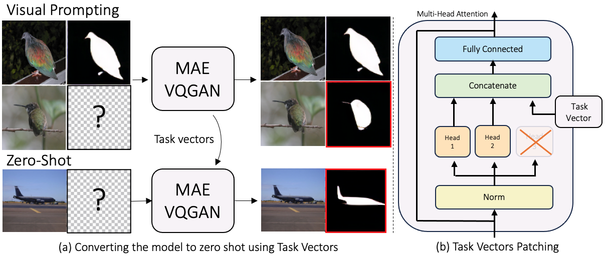
Figure 1: Visual Prompting models like MAE-VQGAN [4] require an input-output example to describe the desired task in their forward pass. We analyze the model activations and find task vectors, activations that encode task information that can be reused to control the task the model performs (see Figure a). Specifically, we tap into activations of individual attention heads and replace their outputs with task vectors to guide the model to the desired task (see Figure b). Surprisingly, the resulting models perform better than the original model while reducing the need for input-output examples. This confirms that task vectors exist in the network activation space and they can guide the model to perform the desired task.

1 Introduction

In-context learning (ICL) is an emergent capability of large neural networks, first discovered in GPT-3 [6]. ICL allows models to adapt to novel downstream tasks specified in the user’s prompt. In computer vision, Visual ICL (known as Visual Prompting [4, 2, 3, 51]) is still at its infancy but it is increasingly becoming more popular due to the appeal of using a single model to perform various downstream tasks without specific finetuning or change in the model weights.

In this work, we ask how in-context learning works in computer vision. While this question has yet to be explored, there has been a significant body of research in Natural Language Processing (NLP) trying to explain this phenomenon [1, 7, 13, 14, 15]. Most recently, Hendel et al.[17] suggested that LLMs encode Task Vectors, these are vectors that can be patched into the network activation space and replace the ICL examples while resulting in a similar functionality. Concurrently, Todd et al. [38] discovered Function Vectors, activations of transformer attention heads that carry task representations. Our work is inspired by these observations and aims to study how ICL works in computer vision.

Can task vectors exist in computer vision models too? To build intuition, we start by exploring the activation space of MAE-VQGAN [4]. Intuitively, we look for intermediate activations that are invariant to changes within a task, but have high variance across different tasks. We use this simple metric to rank activations according to their “taskness”. Estimating this score only requires applying the forward pass of a model over minibatches of data and thus it is very fast to compute. Using this score, we find that the activation space of certain attention heads can perfectly cluster the data by tasks, hinting the existence of visual task vectors.

Based on this insight, we hypothesize that Visual ICL models create task vectors too, and aim to find them. However, finding visual task vectors by relying on previous approaches is challenging. For example, both [17, 38] restricted their search space to the output activations of the last token in the prompt sequence (colored in red in the following example: ‘‘Banana:B, Apple:’’ ). This is natural for text as it is processed sequentially by autoregressive models like LLaMA [39], but with images (see Figure 1, “Visual Prompting” input image), it is not obvious what token activations hold task information, and architectures like MAE-VQGAN [4] do not process image tokens sequentially. This alone increases the search space significantly because multiple tokens might hold task vectors.

To find the set of task vectors, we condition the model on query only (see Figure 1a, bottom row) and search for a subset of mean task activations that can be patched in self attention heads to guide the model towards performing the desired task using REINFORCE [43]. Patching the identified task vectors (see example in Figure 1b) leads to competitive performance with the original model on a range of tasks, which confirms that the set of resulting activations are indeed task vectors. Our approach directly models searching for a subset of activations compared to the previously proposed Casual Mediation Analysis [32] (CMA) that searches each activation independently.

Our contributions are as follows. We show evidence for the existence of visual task vectors and propose a practical way to identify them. Moreover, we find that patching the resulting task vectors guides the model towards the desired task with similar performance compared to the original model while reducing the number of FLOPS by $22.5\%$.

2 Related Work

2.1 Visual Prompting

Visual Prompting [4, 2, 18, 46, 51, 3] is a class of approaches to adapt computer vision models to downstream tasks, inspired by the success of prompting in NLP [6]. Approaches like [2, 18] seek to improve task-specific performance by adding trainable prompt vectors to the model. Other Visual Prompting approaches allow a model to handle various vision tasks [4, 46, 3, 51] by introducing visual examples or text at the time of inference. Such prompting is related to the way in-context learning [45, 42, 22, 25] operates in language models [33, 6, 41]. In fact, trainable prompts and in-context learning can be viewed as two complementary approaches for “describing” a task to a model [21]. Our goal here is to better understand the underlying mechanism of Visual ICL, and we analyze the MAE-VQGAN model presented in [4].

2.2 Explainability

In the context of enhancing model interpretability [50, 29, 37] within computer vision, the integration of Causal Interventions [5, 31] and Activation Patching [48] has become a cornerstone in the elucidation of complex neural networks’ decision-making processes. These methodologies enable a systematic examination of how models encode and utilize high-level concepts, offering profound insights into their internal mechanisms[49, 44, 24]. Causal Interventions [32, 28], facilitate the exploration of the causal structures of models by manipulating their internal states or inputs [12] and observing the impact on outputs, thus uncovering the direct and indirect effects that drive model predictions. Here we use Activation Patching [48] to show through targeted interventions the significance of Task Vectors towards guiding Visual Prompting models to perform different computer vision tasks.

2.3 Task Vectors

In [17, 38, 11], a Task Vector or Function Vector is a latent activation derived from a particular layer of the transformer [40]. This vector subsequently substitutes the original latent states at the same layer during the forward pass of a query to guide the model to perform the desired task. The investigation of Task Vectors aligns with broader efforts in the field to make neural networks more adaptable and tailored to specific tasks [23, 26] as well as boosting the performance [30, 47, 19] by gaining a deeper understanding of how different layers within a model contribute to its overall function. Our work is the first to explore task vectors in computer vision.

3 Methods

Our goal is to understand in-context learning for computer vision, and how existing models can be adapted to different downstream task in inference time. Specifically, we focus on the MAE-VQGAN [4] model, a variant of MAE [16] with a Vision Transformer [9] encoder-decoder architecture.

Given a an input-output example $(x_{s},y_{s})$ and a new query $x_{q}$, to succeed in this ICL task, the model $F$ has to implicitly apply the transformation from $x_{s}$ to $y_{s}$ over $x_{q}$ to produce $y_{q}$:

$$y_{q}=F(x_{s},y_{s},x_{q})$$ (1)

Based on past observations from NLP [17, 38], we hypothesize that computer vision models encode latent task vectors in their activation space during the forward pass as well. This requires the model to implicitly map the input example into a set of latent task vectors $z=\{z_{i}\}^{k}_{i=1}$. Then, the original function $F$ can be decomposed into extracting the task vectors by a function $G$ then applying $F$ on the query while fixing the computed task activations $z$:

$$z=G(x_{s},y_{s}) y_{q}=F(x_{q}|z)$$ (2)

3.1 Scoring Activations

Intuitively, every task vector is an activation that changes across different tasks but remains invariant to changes within a specific task. Specifically, denote $i=(l,m,k)$ as the $l^{th}$ attention block, $m^{th}$ attention head, and $k^{th}$ token and denote it by $F_{i}$ the function that outputs the corresponding activation in the attention block residual stream. We sample an input-output example and a query triplet from individual tasks as well as across tasks and compute the latent activations corresponding to $i$:

$$(x_{s},y_{s},x_{q})\sim\mathbf{D_{all\_tasks}} (x^{\prime}_{s},y^{\prime}_{s},x^{\prime}_{q})\sim\mathbf{D_{task\_j}}$$

$$z^{i}_{all}=F_{i}(x_{s},y_{s},x_{q}) z^{i}_{task_{j}}=F_{i}(x^{\prime}_{s},y^{\prime}_{s},x^{\prime}_{q})$$

Then, we define the score and the mean activations for position $i$ and task $j$:

$${\rho_{token}}(i)=\frac{var(z^{i}_{all})}{{\frac{1}{n}}\sum^{n}_{j=1}var(z^{i}_{task_{j}})} \mu_{i,j}=\mathbb{E}[z^{i}_{task_{j}}]$$ (3)

Table 1: Task Clustering Quality. Clustering Scores of Different Attention Heads, ranked by our Activation Scoring metric (see Section 3). This indicates that higher Activation Scores indeed correlate with better clustering by tasks.

	(Layer, Head)	Our Score	Silhouette Score	Davies-Bouldin Score
		$\uparrow$	$\uparrow$	$\downarrow$
High 1	(26, 3)	2.1663	0.3583	1.2744
High 2	(11, 3)	1.0827	0.2692	1.5567
High 3	(11, 13)	0.9849	0.2246	1.8084
High 4	(22, 3)	0.9448	0.2031	2.6842
Random 1	(4, 3)	0.2329	0.0708	4.1062
Random 2	(18, 16)	0.1259	0.0369	4.3256
Random 3	(32, 6)	0.3253	0.0827	2.9670
Random 4	(11, 14)	0.1196	0.0409	5.3884
Random 5	(18, 16)	0.1259	0.0369	4.3256
Low 1	(2, 16)	0.0221	-0.0518	21.8265
Low 2	(2, 12)	0.0264	-0.0334	13.5982
Low 3	(27, 5)	0.0281	-0.0280	15.4219

Note that since our end goal is to operate in a “zero-shot” setting (e.g, no input-output examples), we only consider the score and task vectors that correspond to the CLS token, the input query, and the output (present in the decoder only). Also, computing the token score and mean activations is very efficient as it simply requires applying the forward pass of a neural network across a batch without any access to a held-out validation set.

Importantly, while $\rho_{token}(\cdot)$ assigns high values to task vectors, it might also assign high values for other potential activations, for example, an activation that captures the color histogram can also vary across tasks (segmentation maps compared to natural images) but remain similar within each individual task. Therefore, we use this scoring mechanism mainly to build intuition about the existence of task vectors.

Finally, we compute the aggregated per-layer score:

$$\rho_{layer}(l)=\sum_{i=(l,m,k)}\rho_{token}(i)$$ (4)

Using this scoring function, we find that some activations capture “taskness” (see Figure 2) and cluster the data well with respect to tasks (see Table 1). We further elaborate on this analysis in Section 4 and Section 5. To find visual task vectors, we leverage a more general approach outlined in the following section.

3.2 Finding Visual Task Vectors via REINFORCE

How can task vectors be identified? An exhaustive search over all subsets of activations is intractable. For example, MAE-VQGAN [4] which we utilize here has $32$ attention blocks, each with $16$ heads, therefore, if we consider these to be the potential set of activations then we need to search over $2^{512}$ options, evaluating each option over a held-out validation set.

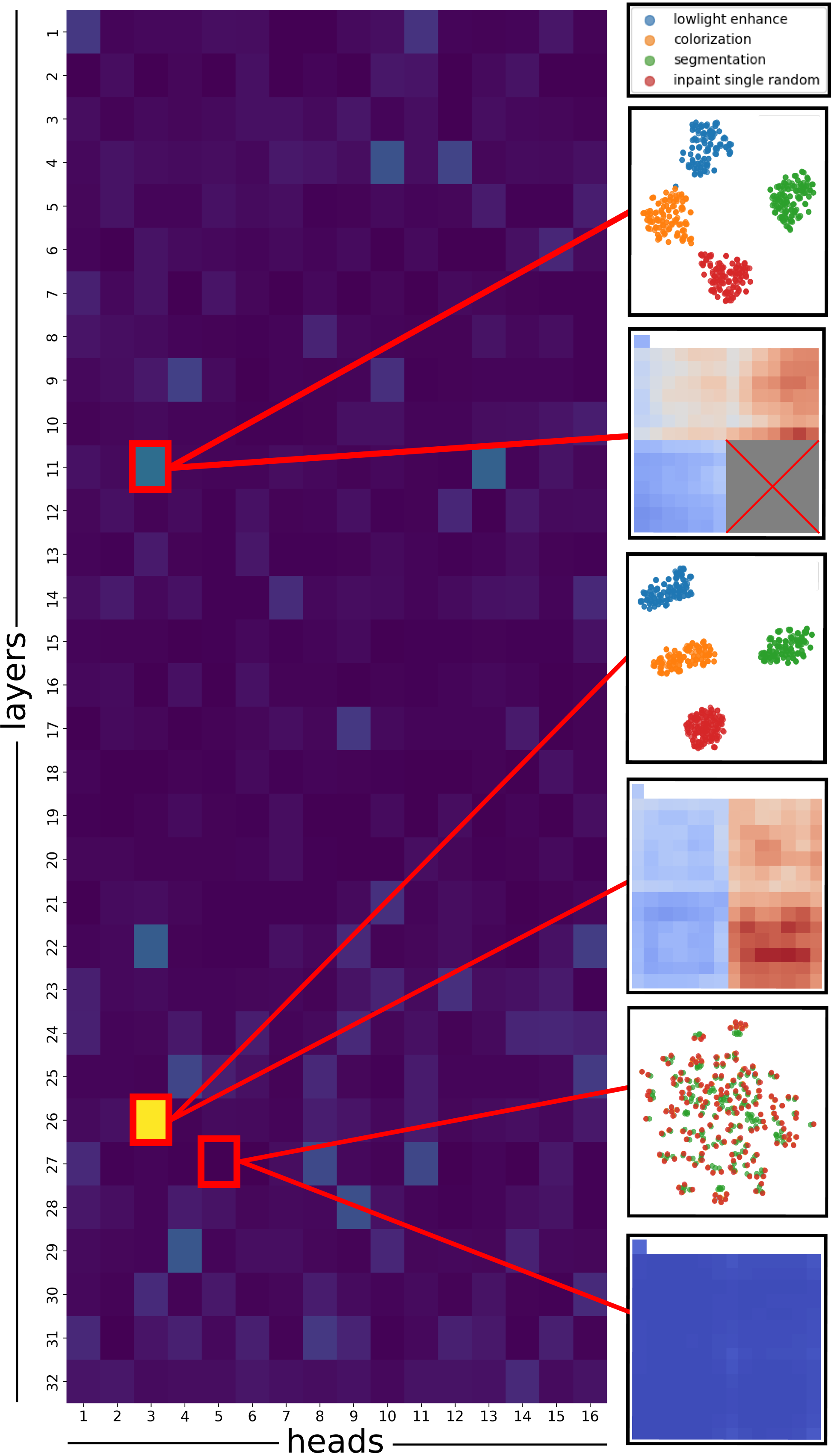
Figure 2: Activation Scoring Analysis. Individual scores (${\rho_{token}}(i)$) aggregated per Attention Head (left). Individual token scores of specific heads are further visualized, along with the t-SNE [27] clustering of head activations of different tasks (right).

For every task $j$ we can apply the following procedure to find the task vectors. Recall that $\{\mu_{i,j}\}$ denote the mean activations and $F(\cdot)$ is a pretrained visual prompting model. Denote $\alpha_{i,j}\sim Bernoulli(\sigma(\theta_{ij}))$ as random variables that signify whether the mean task activation $\mu_{i,j}$ is a task vector and $\theta_{ij}$ is a learned weight followed by the sigmoid function to ensure it is in $[0,1]$.

Denote $z_{j}$ as the set of task vectors for task $j$: $z_{j}=\{\mu_{i,j}|\alpha_{i,j}=1\}$. Given pairs of input-output task demonstrations $x_{q},y_{q}\sim\mathbf{D_{task\_j}}$, we want to find the set of task vectors that minimizes the loss function:

$$L(\theta)=E_{{z_{j}}\sim p_{\theta}}L(y_{q},F(x_{q}|z_{j}))$$ (5)

Where $p_{\theta}$ denotes the sampling distribution of $z_{j}$ and $L$ denotes the loss function that suits the particular task $j$. Note that differently than in Equation 1, if we find a good set of task vectors $z_{j}$, then we no longer need to condition $F$ over additional input-output examples.

To find a set of task vectors, we need to estimate the parameters $\theta$. Since the sampling distribution $p_{\theta}$ depends on $\theta$, it is natural to use the REINFORCE algorithm [43]. The key idea in REINFORCE is the observation that:

$$\nabla L(\theta)=E_{z_{j}\sim p_{\theta}}{L(y_{q},F(x_{q}|z_{j}))\nabla\log p_{\theta}(z_{j})}$$

Thus, we can approximate $\nabla L(\theta)$ by sampling ${z_{j}}$ and averaging the above equation. After iteratively optimizing with gradient descent, we select the final task vector positions by sampling a set of $z_{j}$.

This procedure is outlined for finding the task vectors placements for individual tasks, however it is possible to find placements that generalize for multiple tasks by optimizing over examples across datasets and we refer this as “multi-task” patching. Additionally, while above we search for all token activations, it is possible to apply the search in different levels of granularity. For example, by patching groups of tokens from the same quadrant, patching all the tokens in an attention head, or patching the entire layer. We discuss these design choices in the next section.

4 Experiments

Our experiments aim to explore whether activation patching of task vectors in zero-shot environments can cause the model to execute the desired visual task, hopefully performing similarly–or better–to the original model’s one-shot in-context-learning performance. In this section, we describe the implementation details of MAE-VQGAN, the prompting schemes used, the details of our implementation, the baselines used for comparison, the visual tasks of interest, and the experiments conducted.

4.1 Implementation Details

MAE-VQGAN [4]. An MAE  [16] with a ViT-L [9] backbone, which has $24$ encoder blocks and $8$ decoder blocks, with $16$ attention heads in every layer and a patch size of $16x16$ and input resolution of $224x224$. The decoder predicts a distribution over a VQGAN [10] codebook to output images with better visual quality. We used the pretrained checkpoint from [4] trained over the Computer Vision Figures [4] dataset and ImageNet [35].

One-shot Prompting. We follow the basic one-shot setup in [4]. Specifically, we construct a grid-like image structure with an input-output demonstration, a query, and a masked output region which are embedded into a $2x2$ grid. We feed this grid image to the model to obtain the output prediction which we use for evaluation purposes.

Zero-shot Prompting. Similarly to one-shot with the key difference that only the query is embedded into the grid image, in the same bottom left quadrant position as in the one-shot setting. The model is then used to reconstruct only the part that corresponds to the output. Specifically, we patchify the query image at a resolution of 112x112 and apply to it the positional encodings of the bottom left quadrant. The patches are then fed into the encoder and are processed by the decoder together with the mask tokens that correspond to the bottom right quadrant to obtain the result. Note that in the zero-shot setting we also patch intermediate activations by task vectors.

Causal Mediation Analysis. We compare our methodology with the Causal Mediation Analysis methodology as presented in [38] as a baseline. We select the top 25% of activations with the highest causal score across 10 images.

Greedy Random Search. We compare our methodology to an iterative greedy random search algorithm (GRS) used to select task vectors based on the activation scoring metric proposed in Section 3.1. This serves as a baseline and is outlined in the Supplementary Materials (Section 10.1).

Finding Task Vectors. We use REINFORCE  [43] to select where to patch. We initialize $\theta_{ij}$ with $-1$. Each patch position modeled as a random variable corresponds to either the CLS token, or a grouping of the image patch tokens based on their spatial positioning: the bottom left quadrant (the image patch tokens that correspond to the query), and bottom right quadrant (the MASK tokens). In other words, we restrict the granularity of the patching procedure; instead of having an individual random variable parameter for each token position $i$ we reduce the dimensionality of the search space by grouping the tokens into the three categories mentioned. Upon each iteration of REINFORCE, we sample $32$ times from the Bernoulli distribution for each image (fixed at $10$ for all experiments) and perform a patching procedure into the positions sampled with a value equal to $1$. This results in a total of $320$ executions of zero-shot MAE-VQGAN per iteration. Then, we optimize the Bernoulli parameters as outlined in 3.2 with Adam [20] using a learning rate of $0.1$. We execute the algorithm for a total of $600$ steps and select the checkpoint at intervals of 50 steps with the best evaluation on a held-out test set.

4.2 Activation Scoring Analysis

Here our goal is to evaluate in isolation the Activation Scoring step (outlined in Section 3.1), specifically whether high scoring activations indeed correspond to Task Vectors.

Collecting Activations. As outlined in Section 3.1, our first step towards computing activation scores is to run the forward pass of the model in a one-shot setting to collect activations across different tasks. Specifically, we use $100$ prompts and queries from Pascal 5i [36] training set, ensuring that the one-shot performance across all tasks works reasonably well. During the forward pass, we save the activations for every task $j$ and $i=(l,m,k)$, which corresponds to the intermediate activation of the $k^{th}$ token in the $l^{th}$ block after the $m^{th}$ attention head. Afterwards, we compute the mean activation ${\mu_{i,j}}$ and score $\rho_{token}(i)$.

Evaluation via Clustering. Next, we wish to analyze if $\rho_{token}(i)$ indeed captures “taskness”. Intuitively, we expect layers that capture task information to succeed in clustering activations by task. To assess this, we analyze the clustering performance of vectors with high-ranking activations versus those marked with low scores. We measure the clustering performance using common clustering metrics like the Silhouette Score [34] and the Davies-Bouldin Score [8]. Finally, we also perform a qualitative analysis by visualizing the representations on a t-SNE [27] plot, coloring each data point by it’s task label.

4.3 Downstream Tasks

We evaluate the performance on standard image-to-image tasks like Foreground Segmentation, Low Light Enhancement, In-painting, and Colorization.

Dataset. We use the Pascal-5i [36] dataset, which is comprised of 4 different image splits where every split contains between $346$ and $725$ images and associated segmentation masks. For evaluation, we sample $1000$ prompt-query pairs from each split in the validation set. For Activation Scoring and the various methods to find Task Vectors we only use examples from the training set.

Foreground Segmentation. For model evaluations, we use the segmentation masks included in the Pascal-5i [36] dataset, and report the mean IOU (mIOU) metric across the four splits.

Low Light Enhancement. To obtain the input-output data, given a Pascal-5i [36] image, we multiply the color channels by a factor of $0.5$ and define the result as the input and the original image as the output. We report the Mean Squared Error (MSE) metric of the prediction with the label.

Inpainting. To obtain input-output pairs, we randomly mask a square region in height/width equal to $25\%$ of an image (resulting in a black square of 1/8 the area) and define this as the input, while using the original image as the output. For evaluation, we report the MSE metric.

Colorization. To obtain input-output pairs, we convert an image to grayscale and denote it as the input, and have the output be the original image. For evaluation, we report the MSE metric.

4.4 Ablations

In this section we describe the set of experiments conducted to ascertain the particular implementation details of our REINFORCE [43] method, validating our design choices.

Task Vectors Location in Encoder vs. Decoder. We hypothesize that task implementation occurs in a distributed fashion across multiple parts of the network, necessitating interventions in both the encoder and decoder to induce task implementation in the zero-shot scenario. Hence, we test this by executing our method by restricting interventions to the encoder only, the decoder only, and allowing for interventions throughout the whole network. We report the mIoU on the four splits for the Segmentation task, seeking to find if interventions in both parts of the model are required for appropriate task implementation.

Patching Granularity. We explore different intervention granularities by mapping each token position to a group thus decreasing the dimensionality at which we perform interventions. With this in mind, we can further reduce the size of the search space of the optimization by grouping potential patching positions $i=(l,m,k)$ into spatial quadrants or individual attention heads. We seek to find the optimal granularity at which we maintain precise interventions but manage to reduce the search space nonetheless. We execute our method with three granularity levels (individual tokens, quadrants, attention heads) and report the performance on the four tasks.

4.5 Zero-shot Task Vector Patching

We seek to explore whether zero-shot task vector patching can provide task implementation performance similar to one-shot prompting. We perform the following experiments to investigate this:

Task-specific. For each of the four tasks we execute our task-specific method, and the baselines of Causal Mediation Analysis (CMA) and Greedy Random Search (GRS) with 10 images and report the results on corresponding tasks.

Multi-task. We follow the same procedure but in a multi-task scenario where we select two images and perform our method alongside the CMA and GRS baselines, evaluating the loss across all tasks jointly. We normalize the loss per task in order to account for task-specific differences to ensure no single task dominates the search, and all tasks are weighted equally. Finally, we introduce the identity-copy task to keep the batch size at 10 for equivalent comparisons.

We also provide the following baselines to benchmark the performance of the three algorithms, and to validate the necessity of top $k$ score ranking the layers and performing the iterative search for the GRS method:

MAE-VQGAN. We compare to the original model’s one-shot performance.

Random Quadrants. We patch into randomly sampled positions across the whole network (same total amount of patches as task-specific and multi-task)

GRS across Random K Layers. We execute the search algorithm constraining it to a random set of $k$ layers instead of ranking them by their score. This serves to validate the need of the proposed scoring method.

Patching into Top Quadrants. We patch into the top quadrants based on their scoring (same total amount of patches as task-specific and multi-task). That is, we directly patch into areas with high scores naively without the iterative refining steps of the GRS, to validate its utility.

We report the results across the four splits for the four tasks, and compare all variants to the original MAE-VQGAN model and the random baselines.

5 Results

5.1 Activation Scoring Analysis

We compute ${\rho_{token}}(i)$ and display it aggregated per head on a heatmap where the y-axis is the layer and the x-axis is the attention head index (see Figure 2). This heatmap showcases certain heads that stand out, suggesting that these heads may hold task vectors. From this heatmap we then select the top two heads ranked by score which are at position $(26,3)$ and $(11,3)$; we also select a lower-ranked head at position $(27,5)$. For each of these three heads, we visualize the clustering of its activations, and the individual Activation Score per token. Both are placed to the right side of the heatmap.

Clustering Visualization. We observe a clear clustering based on task in heads ranked highly–head (26,3) for instance–by our scoring methodology, and what appears to be many small clusters for the low-ranked head which we hypothesize are clustering by the semantics of the input prompt-query pair–head (27,5). To perform the dimensionality reduction we vertically stack the activations of a particular head across token positions and project them onto 2D with t-SNE [27] coloring by task.

Score-per-token Heatmap. We display the un-aggregated ${\rho_{token}}(i)$ values for each token re-arranged to convey spatial positioning (equivalent to the 2x2 prompting grid). That is, for the heads of interest, we report the ${\rho_{token}}(i)$ values that the particular individual head encapsulates–displayed on a heatmap. We place the CLS token as the lone square on the top left corner; following this we have the values corresponding to the four different quadrants $(x_{s},y_{s},x_{q},y_{q})$. It is important to note that in the encoder there are no tokens that correspond to the $y_{q}$ (bottom right) quadrant as these are incorporated as mask tokens after the encoder; hence, for visualization purposes we display their value to be marked as X. We observe that within a single head different tokens can take a wide range of values. Interestingly, there appears to be a consistency in values across the tokens in particular quadrants which motivated the decision to group token patching by quadrants.

Quantitative Clustering Analysis. To further support the observation of high and low-quality clustering based off of the scoring value, we report the Silhouette Score and Davies-Bouldin score for the four highest-ranked heads, 5 randomly sampled heads, and the three lowest-ranked heads (see Table 1). We observe that attention heads scored highly by our methodology display high quality clustering scores from the Silhouette Score and Devies-Bouldin Score and vice-versa for those scored lowly. Finally, the randomly selected attention heads received intermediate scores.

5.2 Zero-shot Task Vector Patching

We now share the performance of our method, both task-specific and multi-task, in comparison to the original model and the following baselines: Causal Mediation Analysis, Greedy Random Search, Random Quadrants, Random K Layers, and Top Quadrants. Surprisingly, by performing these interventions with task vectors we are able to implement visual ICL tasks with better performance than the original model. We observe in the following Table  2 (which displays the mean and variance across the 4 splits, or Table 5 in the Supplementary Materials which contains the individual split evaluations), that our task-specific models beat the original MAE-VQGAN across all tasks. Furthermore, the GRS task-specific models beat the original MAE-VQGAN in some tasks. We also observe that our multi-task models beat the original MAE-VQGAN in all tasks except Segmentation where performance is met, and GRS multi-task performs comparably to the original. CMA performs better than the random baselines but does not reach the high performance of our method, or the GRS method nonetheless.

Furthermore, we provide validation that ranking layers by their $\rho_{layer}(l)$ and selecting the top-k is instrumental to supporting the performance of the greedy random search by comparing to randomly selecting k layers. We see that random K layers does not perform well, except for colorization where it is similar to GRS. Moreover, if we simply patch into the top quadrants without the GRS we get poor performance.

Table 2: Quantitative Analysis. Results comparison across different tasks and splits, indicating the effectiveness of our task-specific model.

	Segmentation $\uparrow$	Lowlight Enhance $\downarrow$	Colorization $\downarrow$	In-painting $\downarrow$
Model	(Mean ± STD)	(Mean ± STD)	(Mean ± STD)	(Mean ± STD)
Original MAE-VQGAN	$0.338\pm 0.033$	$0.685\pm 0.032$	$0.618\pm 0.027$	$0.550\pm 0.042$
Random Quadrants	$0.170\pm 0.061$	$3.000\pm 0.967$	$3.025\pm 1.190$	$2.350\pm 0.955$
Random K Layers	$0.090\pm 0.007$	$1.825\pm 0.043$	$0.568\pm 0.022$	$0.875\pm 0.100$
Top Quadrants	$0.150\pm 0.023$	$4.875\pm 0.228$	$4.250\pm 0.269$	$3.900\pm 0.141$
CMA (Task-specific)	$0.230\pm 0.012$	$0.825\pm 0.043$	$0.895\pm 0.063$	$1.750\pm 0.112$
CMA (Multi-task)	$0.150\pm 0.017$	$1.400\pm 0.122$	$1.130\pm 0.075$	$1.225\pm 0.083$
GRS (Task-specific)	$0.320\pm 0.021$	$0.600\pm 0.025$	$0.555\pm 0.025$	$0.580\pm 0.047$
GRS (Multi-task)	$0.323\pm 0.019$	$0.515\pm 0.032$	$0.568\pm 0.029$	$0.605\pm 0.036$
Ours (Multi-task)	$0.325\pm 0.026$	$0.492\pm 0.025$	$0.502\pm 0.036$	$0.558\pm 0.022$
Ours (Task-specific)	$\textbf{0.353}\pm 0.028$	$\textbf{0.458}\pm 0.032$	$\textbf{0.453}\pm 0.036$	$\textbf{0.480}\pm 0.022$

We now share the qualitative results for Segmentation, Lowlight Enhancement, and In-painting. First, we visualize the task-specific models of our methodology alongside the original MAE-VQGAN, and the CMA and GRS baselines (see Figure 3). Secondly, we visualize the task-specific and multi-task variants of our methodology in comparison to CMA and GRS(see Figure 4)

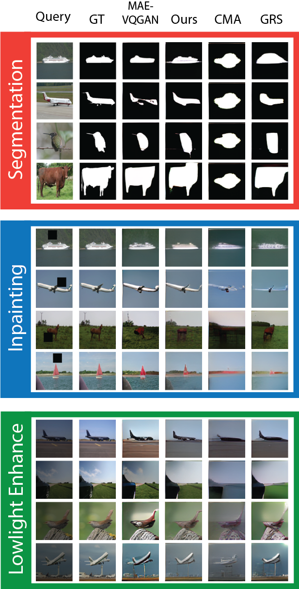
Figure 3: Qualitative Examples. We qualitatively compare the task-specific variants of our methodology’s results with the original model and the CMA and GRS baselines. Our patching methodology performs better than the original MAE-VQGAN model.

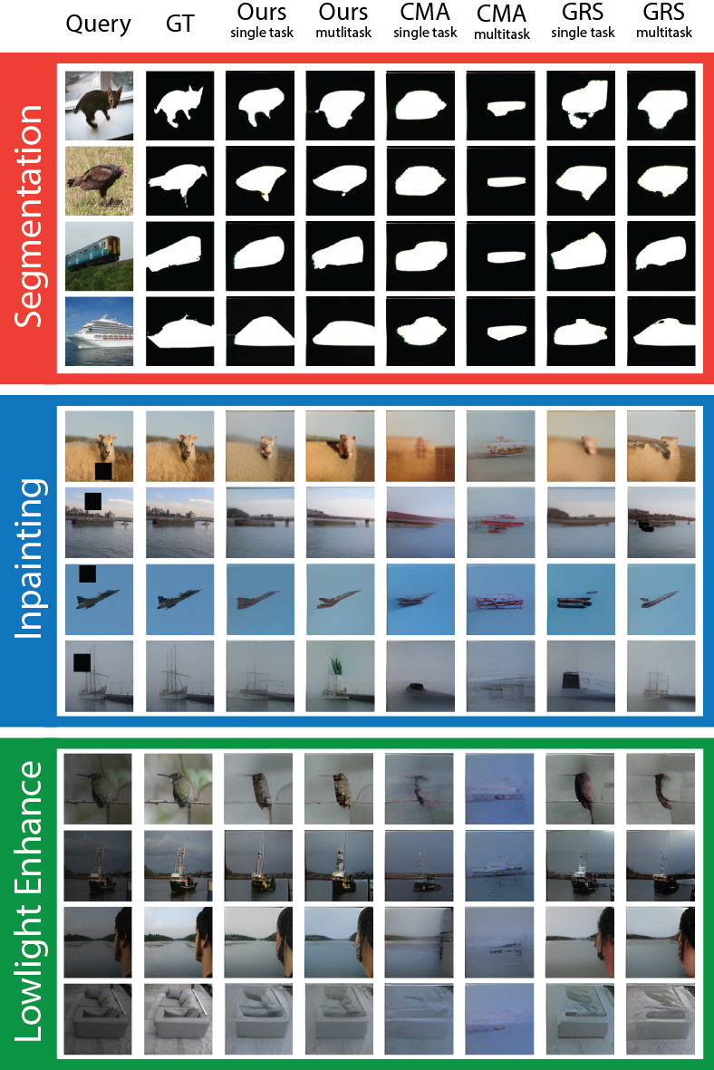
Figure 4: Qualitative Examples. We qualitatively compare the task-specific and multi-task variants of our methodology with the CMA and GRS baselines. Our patching methodology performs better than the original MAE-VQGAN model.

5.3 Ablations

Task Vectors Location in Encoder vs. Decoder. We report our results on isolating the set of possible interventions to the encoder only, decoder only, in contrast to allowing interventions throughout the whole network. We can observe that in-context task learning builds upon both model components. The decoder, however, is more important. It is clear that intervening in both components is crucial for task implementation as we hypothesize that it is computed in a distributed fashion with cascading higher-order effects through the network where early interventions have strong downstream effects (see Table 3).

Table 3: Isolating Task Locations. Patching into Encoder only, Decoder only, and both.

	Segmentation $\uparrow$
Model	Split 0	Split 1	Split 2	Split 3
Encoder (Task-specific)	0.09	0.14	0.14	0.13
Decoder (Task-specific)	0.32	0.34	0.29	0.29
Both (Task-specific)	0.35	0.35	0.31	0.29

Patching Granularity. Motivated by the emergence of quadrants in the per-token scoring visualization, we explore the optimal granularity at which to group the tokens to reduce the dimensionality of the search space. In the tasks of Segmentation and Colorization, grouping by quadrants results in better performance; whereas in the tasks of Lowlight Enhancement and In-painting, maintaining full patching granularity at the token level results in better performance (see Table 4 which displays the mean and variance across the 4 splits, or Table 6 in the Supplementary Materials which contains the individual split evaluations).

Table 4: Optimal Patching Granularity. Patching into Tokens (T), Quadrants (Q), or Heads (H)

	Segmentation $\uparrow$	Lowlight Enhance $\downarrow$	Colorization $\downarrow$	In-painting $\downarrow$
Model	(Mean ± STD)	(Mean ± STD)	(Mean ± STD)	(Mean ± STD)
Ours T (Task-specific)	$\textbf{0.350}\pm 0.025$	$0.495\pm 0.036$	$\textbf{0.453}\pm 0.036$	$0.485\pm 0.018$
Ours Q (Task-specific)	$0.338\pm 0.023$	$\textbf{0.458}\pm 0.032$	$0.465\pm 0.036$	$\textbf{0.480}\pm 0.022$
Ours H (Task-specific)	$0.245\pm 0.015$	$0.942\pm 0.070$	$0.857\pm 0.069$	$0.885\pm 0.067$
Ours T (Multi-task)	$0.318\pm 0.023$	$0.510\pm 0.028$	$0.510\pm 0.039$	$0.565\pm 0.025$
Ours Q (Multi-task)	$\textbf{0.325}\pm 0.026$	$\textbf{0.492}\pm 0.025$	$\textbf{0.502}\pm 0.036$	$\textbf{0.558}\pm 0.022$
Ours H (Multi-task)	$0.253\pm 0.013$	$1.105\pm 0.064$	$0.998\pm 0.069$	$0.980\pm 0.082$

6 Limitations

Our focus was in identifying Task Vectors, but we hypothesize that there might exist other important vector-types such as image structure activations that capture locations, input-output placements, and left-to-right ordering. During the optimization with REINFORCE [43] we evaluate the performance using the MSE metric for all tasks (except Segmentation which uses mIoU) after decoding the predicted VQGAN tokens. Instead, it may be possible to directly evaluate the model in VQGAN token space using cross entropy loss which may lead to more accurate results. We leave these extensions for future works.

7 Conclusion

In this work we explore the internal mechanisms of visual in-context learning and devise an algorithm to identify Task Vectors, activations present in transformers that can replace the in-context examples to guide the model into performing a specific task. We confirm our approach by adapting MAE-VQGAN to perform specific tasks in a zero-shot fashion by patching the Task Vector identified. We find that different than in NLP, in computer vision Task Vectors are distributed throughout the network’s encoder and decoder.

Acknowledgements: This project has received funding from the European Research Council (ERC) under the European Unions Horizon 2020 research and innovation programme (grant ERC HOLI 819080). Prof. Darrell’s group was supported in part by DoD including DARPA’s LwLL and/or SemaFor programs, as well as BAIR’s industrial alliance programs.

Supplementary Material

8 Full Results

As supplementary material, we provide the tables displaying the full evaluations across the 4 splits of our method alongside the baselines, and the different patching granularities.

Table 5: Quantitative Analysis. Results comparison across different tasks and splits, indicating the effectiveness of our task-specific model.

	Segmentation $\uparrow$				Lowlight Enhancement $\downarrow$
Model	Split 0	Split 1	Split 2	Split 3	Split 0	Split 1	Split 2	Split 3
Original MAE-VQGAN	0.35	0.38	0.33	0.29	0.70	0.66	0.73	0.65
Random Quadrants	0.08	0.25	0.16	0.19	4.30	2.40	3.50	1.80
Random K Layers	0.09	0.10	0.09	0.08	1.80	1.80	1.90	1.80
Top Quadrants	0.11	0.17	0.16	0.16	4.50	5.00	5.10	4.90
CMA (Task-specific)	0.23	0.25	0.22	0.22	0.76	0.83	0.88	0.83
CMA (Multi-task)	0.18	0.14	0.14	0.14	1.2	1.5	1.5	1.4
GRS (Task-specific)	0.33	0.35	0.30	0.30	0.56	0.61	0.63	0.60
GRS (Multi-task)	0.33	0.35	0.31	0.30	0.47	0.52	0.56	0.51
Ours (Multi-task)	0.35	0.35	0.31	0.29	0.46	0.49	0.53	0.49
Ours (Task-specific)	0.38	0.38	0.33	0.32	0.41	0.46	0.50	0.46

	Colorization $\downarrow$				In-painting $\downarrow$
Model	Split 0	Split 1	Split 2	Split 3	Split 0	Split 1	Split 2	Split 3
Original MAE-VQGAN	0.59	0.62	0.66	0.60	0.49	0.55	0.61	0.55
Random Quadrants	2.10	4.10	4.30	1.60	3.80	1.20	1.90	2.50
Random K Layers	0.54	0.57	0.60	0.56	0.72	0.89	1.00	0.89
Top Quadrants	3.80	4.40	4.30	4.50	3.70	3.90	4.10	3.90
CMA (Task-specific)	0.79	0.92	0.96	0.91	1.6	1.8	1.9	1.7
CMA (Multi-task)	1.02	1.2	1.2	1.1	1.1	1.3	1.3	1.2
GRS (Task-specific)	0.52	0.56	0.59	0.55	0.52	0.56	0.65	0.59
GRS (Multi-task)	0.53	0.57	0.61	0.56	0.55	0.61	0.65	0.61
Ours (Multi-task)	0.45	0.51	0.55	0.50	0.53	0.56	0.59	0.55
Ours (Task-specific)	0.40	0.46	0.50	0.45	0.45	0.49	0.51	0.47

Table 6: Optimal Patching Granularity. Patching into Tokens (T), Quadrants (Q), or Heads (H)

	Segmentation $\uparrow$				Lowlight Enhancement $\downarrow$
Model	Split 0	Split 1	Split 2	Split 3	Split 0	Split 1	Split 2	Split 3
T (Task-specific)	0.38	0.37	0.33	0.32	0.44	0.50	0.54	0.50
Q (Task-specific)	0.36	0.36	0.32	0.31	0.41	0.46	0.50	0.46
H (Task-specific)	0.24	0.27	0.23	0.24	0.83	0.97	1.02	0.95
T (Multi-task)	0.34	0.34	0.30	0.29	0.47	0.51	0.55	0.51
Q (Multi-task)	0.35	0.35	0.31	0.29	0.46	0.49	0.53	0.49
H (Multi-task)	0.26	0.27	0.24	0.24	1.01	1.12	1.19	1.10

	Colorization $\downarrow$				In-painting $\downarrow$
Model	Split 0	Split 1	Split 2	Split 3	Split 0	Split 1	Split 2	Split 3
T (Task-specific)	0.40	0.46	0.50	0.45	0.46	0.49	0.51	0.48
Q (Task-specific)	0.41	0.47	0.51	0.47	0.45	0.49	0.51	0.47
H (Task-specific)	0.75	0.88	0.94	0.86	0.78	0.92	0.96	0.88
T (Multi-task)	0.45	0.51	0.56	0.52	0.53	0.57	0.60	0.56
Q (Multi-task)	0.45	0.51	0.55	0.50	0.53	0.56	0.59	0.55
H (Multi-task)	0.89	1.02	1.08	1.0	0.85	1.02	1.07	0.98

9 More Qualitative Examples

We provide a wider selection of examples comparing our zero-shot task vector patching methodology in comparison to 1) the original one-shot MAE-VQGAN, CMA, and GRS, and 2) our ablations. Alongside each figure, we accompany it with an according analysis.

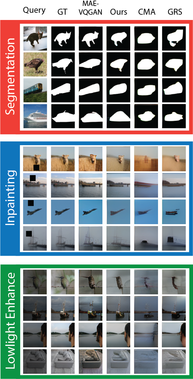
Figure 5: Qualitative Examples. We qualitatively compare our the task-specific variants of our methodology with the original model and the CMA and GRS baselines.

First, we visualize the task-specific models of our methodology alongside the original MAE-VQGAN, and the CMA and GRS baselines (see Figure 5). Secondly, we visualize the task-specific and multi-task variants of our methodology in comparison to CMA (see Figure 6).

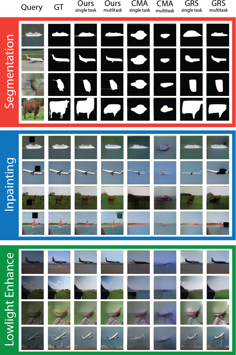
Figure 6: Qualitative Examples. We qualitatively compare the task-specific and multi-task variants of our methodology with the CMA and GRS baselines.

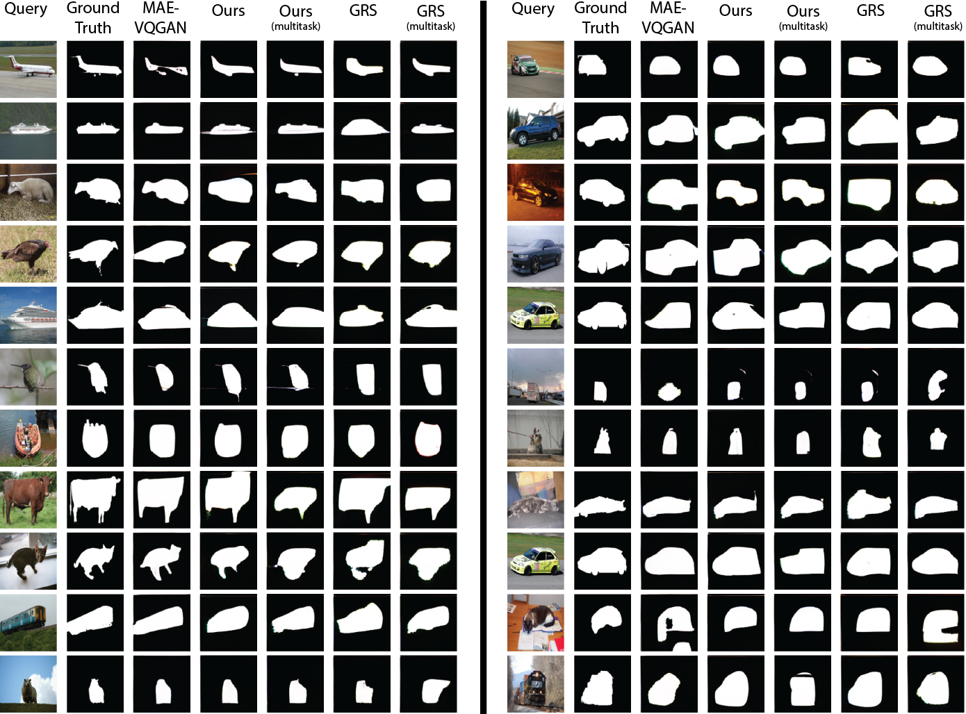
Figure 7: Our Results on Segmentation Task

Qualitative Analysis for Segmentation. In Figure 7, we compare our methodology and GRS task-specific and multi-task methods to the original one-shot MAE-VQGAN performance on the task of Segmentation. It appears that our method is good at segmenting the coarse and fine details of the object of focus. In many cases, the segmentations generated by the original MAE-VQGAN suffer from holes or incomplete masks. In contrast, our method outputs consistent and coherent masks. On the other hand, the GRS method suffers with particular details especially observable when attempting to segment an animal’s ear or leg. However, in many such cases it performs better than MAE-VQGAN at getting the general shape of objects.

Qualitative Analysis for Lowlight Enhancement. In Figure 8, we compare our methodology and GRS task-specific and multi-task methods to the original one-shot MAE-VQGAN performance on the task of Lowlight Enhancement. It appears that the GRS method suffers in maintaining the visual qualities of the query image. However there are many cases where MAE-VQGAN assigns bright colors which is likely due to the particular prompt in use and the inherent ambiguities of the task. On the other hand, our method–particularly the multi-task variant–ouputs consistently better results with accurate visual qualities. In some cases our method produces somewhat muted or blurry results which may be a consequence of using MSE in the pixel space as supervision, but nonetheless reports better quantitative performance.

Qualitative Analysis for In-painting. In Figure 9, we compare our methodology and GRS task-specific and multi-task methods to the original one-shot MAE-VQGAN performance on the task of In-painting. We observe that our method consistently outperforms the original model. However, it appears that the GRS task-vector patching method–once again–suffers in maintaining the higher frequency components of the query image; it appears to reduce the contrast of the image and reduce saturation. However, there are many such cases where the original MAE-VQGAN one-shot technique fails to appropriately implement the task while our method succeeds. The original model’s performance depends heavily on the specific prompt used which may be the root cause of failures while task-vector patching succeeds.

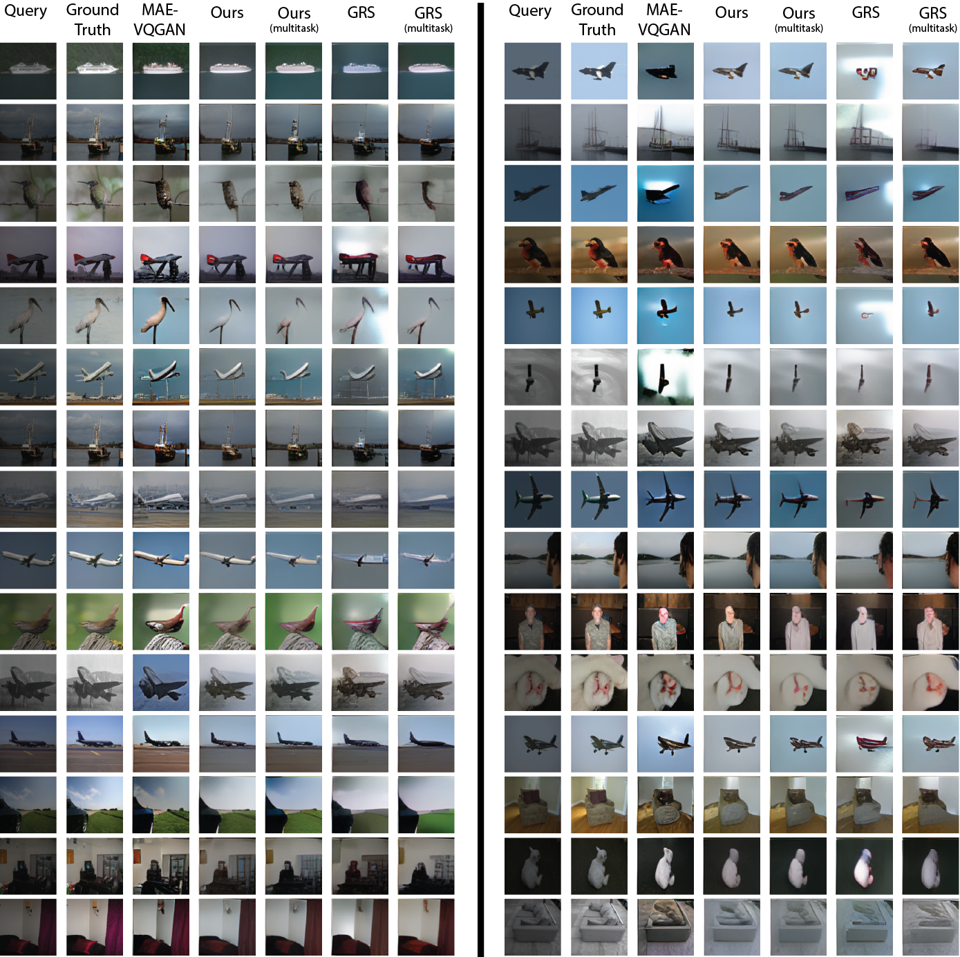
Figure 8: Our Results on Lowlight Enhancement Task

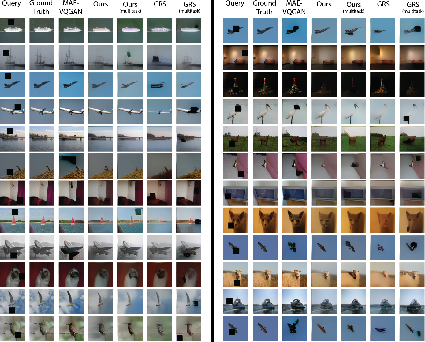
Figure 9: Our Results on In-painting Task

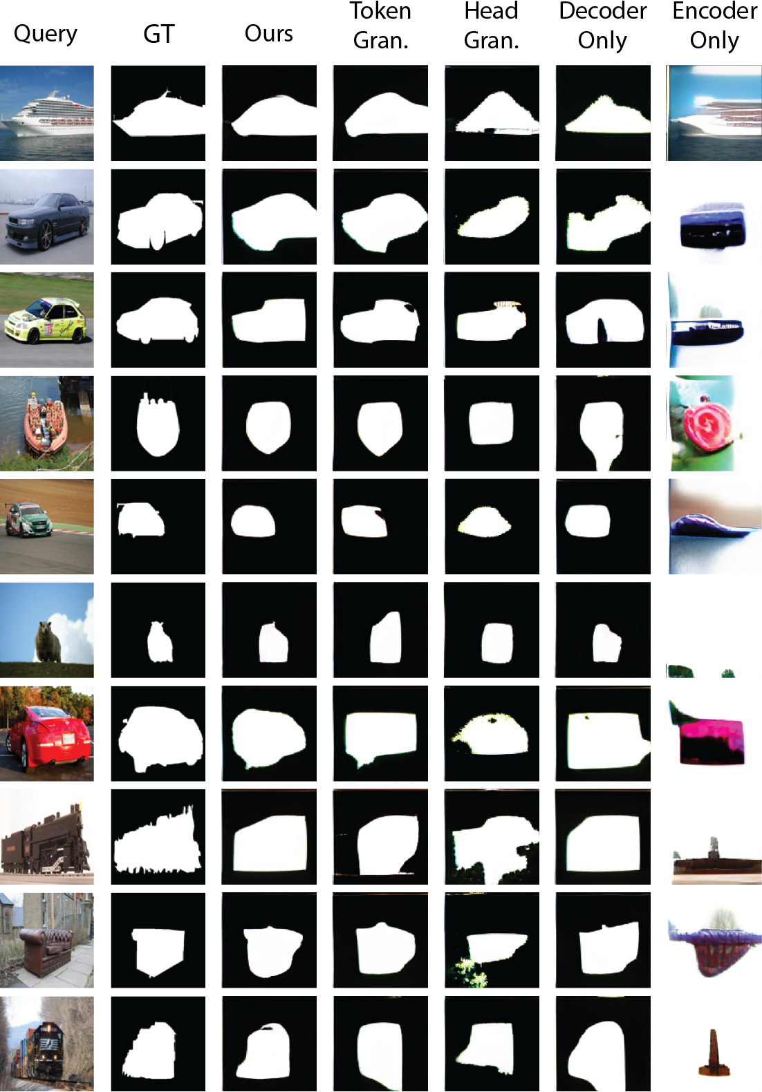
Figure 10: REINFORCE Ablations for Segmentation Task

Qualitative Analysis of Ablations. Finally, we present the qualitative analysis of the different ablations for the Segmentation task in Figure 10. The benefits of observing the visual features of the different ablations in addition to quantitative analysis becomes clear when comparing the Decoder Only and Encoder Only columns. Here it is clear that patching into decoder is of utmost importance in relation to patching into the encoder; the distinction is clear when observing qualitative features. In the end, it is both parts in synchrony which allow for the implementation of in-context learning.

10 Greedy Random Search baseline

10.1 Selecting Task Vectors via Greedy Random Search

For every task $j$ we apply the following algorithm to obtain a task-specific model.

Input. The mean activations $\{\mu_{i,j}\}$, scoring function $\rho_{layer}(\cdot)$, pretrained visual prompting model $F(\cdot)$, and an evaluation set.

Initialization. Initialize a set of binary indicators $\{\alpha_{i,j}\}$ for all $i$, where $\alpha_{i,j}\in\{0,1\}$ signifies whether the mean task activation $\mu_{i,j}$ is a task vector. Next we describe the algorithm to choose the values of $\alpha_{i,j}$.

For every activation $i=(l,m,k)$ in the top $k$ scoring layers w.r.t $\rho_{layer}(l)$, randomly choose the value of $\alpha_{i}$ by sampling from a Bernoulli random variable with parameter value $p$. Set the activation vectors to be $z_{j}=\{\mu_{i,j}|\forall ij~{}\text{if}~{}\alpha_{i,j}=1\}$. Evaluate the now task-specific model $F(\cdot|z_{j})$ on a held-out validation set. Run for $T$ trials and for every $i,j$ set the values of $\alpha_{i,j}$ to be the values from the most successful trial.

Greedy Search. Iterate over $l$ in the top $k$ scoring layers sorted by $\rho_{layer}(l)$ from high to low, pick activation $i=(l,m,k)$, flip the value $\alpha_{i,j}$ and evaluate the validation score for $F(\cdot|z_{j})$. After having evaluated each flip of the $\alpha_{i,j}$ on the particular layer $l$ we keep the $\alpha_{i,j}$ which performed best or continue to the next layer if the performance did not improve.

Termination. When one search loop across the $k$ layers results in no changes - or after $10k$ iterations, the search has thus converged and we return the single-task model $F(\cdot|z_{j})$.

This procedure is outlined for every token, attention head, and layer. However, it is possible to apply it in different levels of granularity. For example, by patching group of tokens from the same quadrant, patching all the tokens in an attention head, or patching the entire layer. We discuss these design choices in the next section.

10.2 Greedy Random Search Implementation Experiments

In this section we describe the set of experiments conducted to ascertain the particular implementation details of the greedy random search, validating the design choices.

Implementation Details We search through the top $k=17$ layers ranked by Activation Scoring. During the initialization phase we sample $\alpha_{i,j}\in\{0,1\}$ from a Bernoulli distribution with a parameter of $p=0.3$ (probability of selecting 1) and evaluate performance. We repeat this for $T=100$ trials and continue with the best performing $\alpha_{i,j}$. Furthermore, we perform a grouping of token positions $i$ in each individual attention head into 3 groups: the CLS token, bottom left quadrant, and bottom right quadrant. This serves to further reduce the search space. We use a set of 10 training images to supervise the search. These design decisions are further validated through ablation experiments.

Selecting Initialization Parameters. For the initialization of the Greedy Random Search there are two parameters, $k$ which dictates how many layers to search across and the Bernoulli random variable parameter $p$ which dictates the probability at which we set $\alpha_{i,j}$ to be 1 during the initialization phase. The question is, which $k$ value is best at narrowing down the search space without restricting our ability to induce task implementation, and what is the best according $p$ value? We ascertain this by searching for the optimal configuration to initialize the Greedy Random Search. We perform a grid search for $k$ values from 14 to 20, and $p$ values from 0.1 to 0.6 and report the evaluation metric for the Segmentation task on the batch of 10 images. Our goal is to find the $(k,p)$ pair with highest performing random initialization.

Task Vectors Location in Encoder vs. Decoder. Similar to the ablation conducted for our main methodology (via REINFORCE [43]) implementation, we execute the Greedy Random Search for the Segmentation task by restricting interventions to the encoder only, the decoder only, and allowing for interventions throughout the whole network. It is key to note that in order to restrict interventions to the decoder only, which has 8 layers, the $k$ value must be set to 8, whereas for isolating the encoder we can keep the original $k=17$ value. We report the mIoU on the four splits for the Segmentation task seeking to find if interventions in both parts of the model are required for appropriate task implementation.

Patching Granularity. We execute our Greedy Random Search with three granularity levels, grouping by Quadrants, grouping by Heads, and grouping by Layers, and report the mIoU performance on the four splits for the Segmentation task.

10.3 GRS Implementation Experiments Results

Selecting K. We explore the optimal parameters for a random initialization. We find the best setup to be to constrain the search across the top $k=17$ layers, sampling quadrants to patch with a probability of $p=0.3$ (see Figure 11).

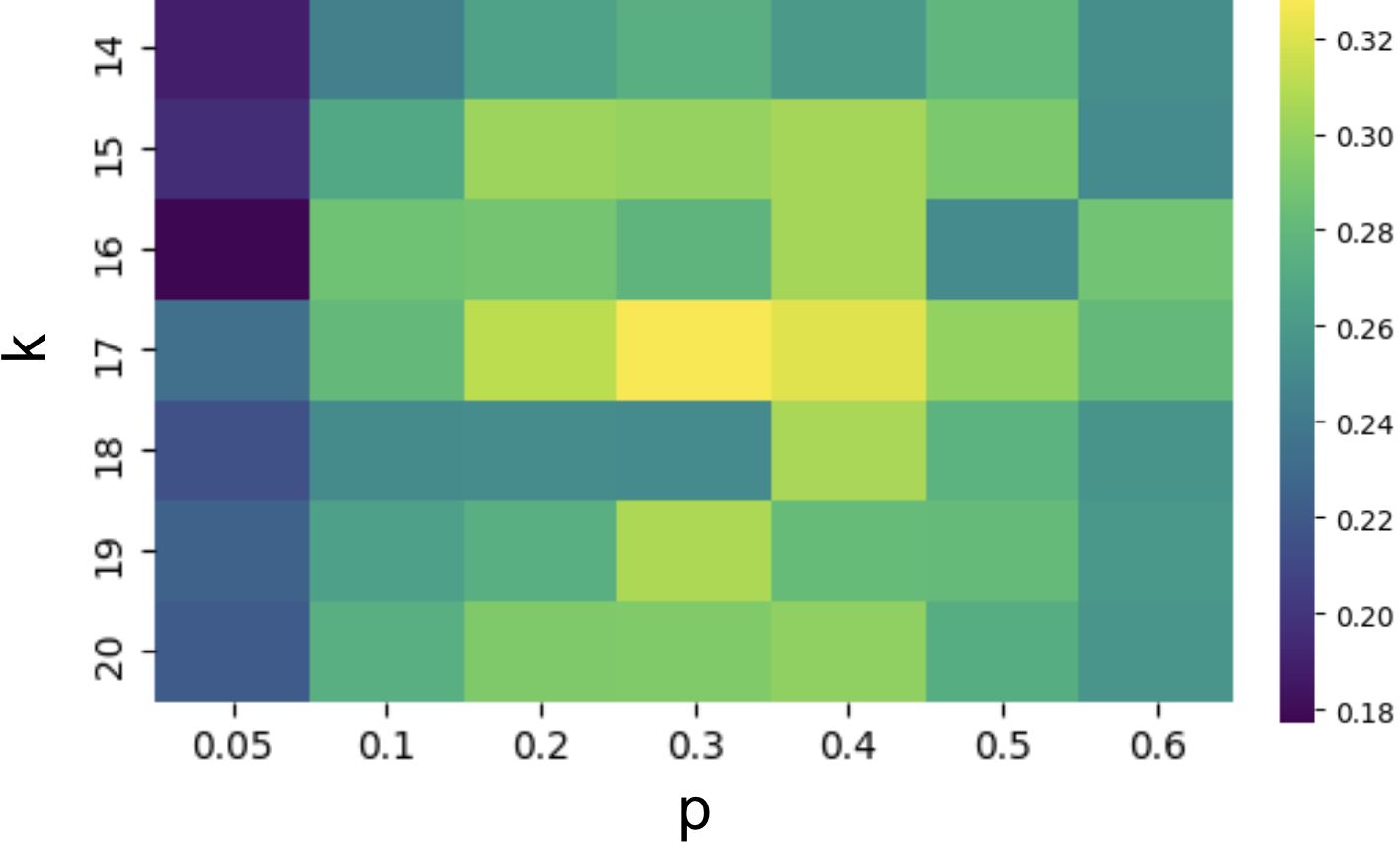
Figure 11: Selecting Initialization Parameters. We evaluate Foreground Segmentation mIoU on Pascal 5i using $10$ images for different random initialization parameterized by $K$ and $p$.

Task Vectors Location in Encoder vs. Decoder. We report the results on isolating the set of possible interventions to the encoder only, decoder only, in contrast to allowing interventions throughout the whole network. We can observe that in-context task learning builds upon both model components. The decoder, however, is more important. It is clear that intervening in both components is crucial for task implementation as we hypothesize that it is computed in a distributed fashion with cascading higher-order effects through the network where early interventions have strong downstream effects (see Table 8).

Table 7: Isolating Task Locations. Patching into Encoder only, Decoder only, and Both

	Segmentation $\uparrow$
Model	Split 0	Split 1	Split 2	Split 3
GRS Both (Task-specific)	0.33	0.35	0.30	0.30
GRS Encoder (Task-specific)	0.13	0.22	0.20	0.20
GRS Decoder (Task-specific)	0.26	0.28	0.25	0.25

Table 8: Optimal Patching Granularity. Patching into Full Layers, Full Heads, or Quadrants only

	Segmentation $\uparrow$
Model	Split 0	Split 1	Split 2	Split 3
GRS Quadrants (Task-specific)	0.33	0.35	0.30	0.30
GRS Heads (Task-specific)	0.15	0.15	0.14	0.13
GRS Layers (Task-specific)	0.28	0.31	0.26	0.27

Patching Granularity. We explore the optimal granularity at which to group the tokens to reduce the dimensionality of the search space. Motivated by the emergence of quadrants in the per-token scoring visualization, and validated by attempting to group by whole attention heads (patching into all the tokens in the attention head) and group by whole layers (patching into all the attention heads of a layer), it is clear that quadrants provide the best trade-off between reducing the dimensionality of the search space and performance (see Table 8). It is interesting to note that patching into full layers reduces the search space to a size of $2^{\text{32}}$ whereas attention heads is $2^{\text{512}}$ and quadrants is $2^{\text{768}}$ for the encoder and $2^{\text{384}}$ in the decoder (disregarding top-k layer selection).

10.4 GRS Baseline Qualitative Comparisons

We provide a wider selection of examples comparing our GRS zero-shot task vector patching methodology in comparison to 1) a selection of baselines, and 2) our ablations. Alongside each figure, we accompany it with an according analysis.

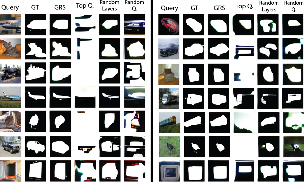
Figure 12: GRS Baseline Comparison for Segmentation

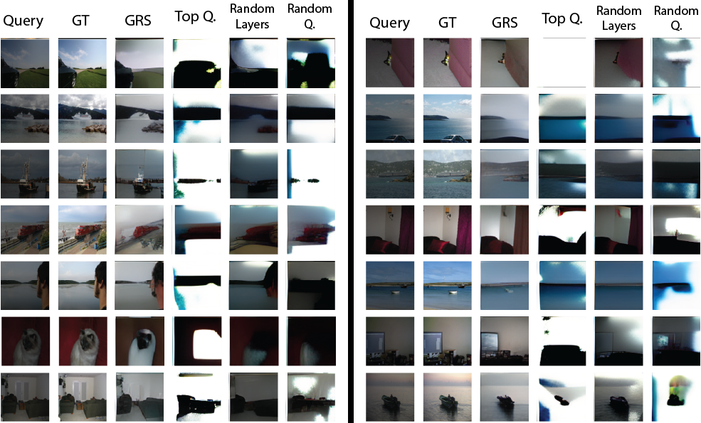
Figure 13: GRS Baseline Comparison for Low light Enhancement

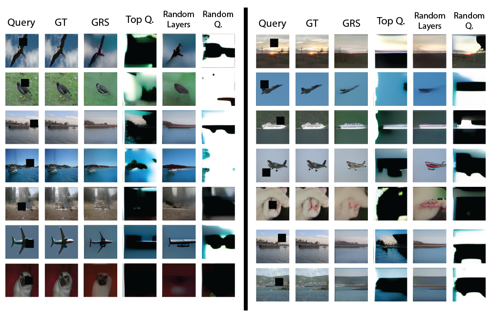
Figure 14: GRS Baseline Comparison for In-painting

In the Figures 12, 13, and 14 we compare our GRS task-specific method with a handful of baselines defined in section 4.5. We have abbreviated Top Quadrants as Top Q, Random K Layers as Random Layers, and Random Quadrants as Random Q. It is clear that Top Quadrants struggles to output coherent completions. We believe this to be because of the need of patching into positions of different purposes other than task implementation such as positions that encode the input-output structure that a one-shot prompt provides. Further opportunities for exploration could include other scoring terms that take into account structural information provided by different prompt orientations. Random K Layers performs surprisingly well due to the efficiency of the Greedy Random Search but nonetheless does not reach the performance of using our scoring mechanism to select the top $K$ layers. Finally Random Quadrants struggles to complete coherent results.

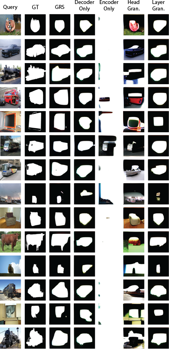
Figure 15: GRS Ablation for Segmentation Task

Finally, we present the qualitative analysis of the different ablations for the Segmentation task in Figure 15. Similarly to our main method (via REINFORCE [43]), it is clear that patching into decoder is more important than patching into the encoder but in the end, it is both parts in synchrony which report the best performance. Furthermore, it is clear that the optimal granularity for patching is at a quadrant level. We find it counterintuitive that layer-level patching performs better than head-level patching–as one would assume that a finer granularity provides better accuracies. However, we believe that by grouping per-layer we significantly reduce the search space (by a factor of 16) which reduces the probability of falling into a local optimum; whereas grouping by head, we suffer from a reduced precision but do not gain the benefits of a reduced search space magnitude (factor of 2 for encoder and factor of 3 for decoder when grouping by head instead of 16 when grouping by layer). Further exploration in this direction is of interest.

References

- [1] Akyürek, E., Schuurmans, D., Andreas, J., Ma, T., Zhou, D.: What learning algorithm is in-context learning? investigations with linear models. arXiv preprint arXiv:2211.15661 (2022)
- [2] Bahng, H., Jahanian, A., Sankaranarayanan, S., Isola, P.: Exploring visual prompts for adapting large-scale models. arXiv preprint arXiv:2203.17274 (2022)
- [3] Bai, Y., Geng, X., Mangalam, K., Bar, A., Yuille, A., Darrell, T., Malik, J., Efros, A.A.: Sequential modeling enables scalable learning for large vision models. arXiv preprint arXiv:2312.00785 (2023)
- [4] Bar, A., Gandelsman, Y., Darrell, T., Globerson, A., Efros, A.: Visual prompting via image inpainting. Advances in Neural Information Processing Systems 35, 25005–25017 (2022)
- [5] Bau, D., Zhu, J.Y., Strobelt, H., Zhou, B., Tenenbaum, J.B., Freeman, W.T., Torralba, A.: Gan dissection: Visualizing and understanding generative adversarial networks. arXiv preprint arXiv:1811.10597 (2018)
- [6] Brown, T., Mann, B., Ryder, N., Subbiah, M., Kaplan, J.D., Dhariwal, P., Neelakantan, A., Shyam, P., Sastry, G., Askell, A., et al.: Language models are few-shot learners. Advances in neural information processing systems 33, 1877–1901 (2020)
- [7] Dai, D., Sun, Y., Dong, L., Hao, Y., Sui, Z., Wei, F.: Why can gpt learn in-context? language models secretly perform gradient descent as meta optimizers. arXiv preprint arXiv:2212.10559 (2022)
- [8] Davies, D., Bouldin, D.: A cluster separation measure. Pattern Analysis and Machine Intelligence, IEEE Transactions on PAMI-1, 224 – 227 (05 1979). https://doi.org/10.1109/TPAMI.1979.4766909
- [9] Dosovitskiy, A., Beyer, L., Kolesnikov, A., Weissenborn, D., Zhai, X., Unterthiner, T., Dehghani, M., Minderer, M., Heigold, G., Gelly, S., Uszkoreit, J., Houlsby, N.: An image is worth 16x16 words: Transformers for image recognition at scale (2021)
- [10] Esser, P., Rombach, R., Ommer, B.: Taming transformers for high-resolution image synthesis. In: Proceedings of the IEEE/CVF Conference on Computer Vision and Pattern Recognition (CVPR). pp. 12873–12883 (June 2021)
- [11] Ferry, Q.R., Ching, J., Kawai, T.: Emergence and function of abstract representations in self-supervised transformers. arXiv preprint arXiv:2312.05361 (2023)
- [12] Gandelsman, Y., Efros, A.A., Steinhardt, J.: Interpreting clip’s image representation via text-based decomposition. arXiv preprint arXiv:2310.05916 (2023)
- [13] Garg, S., Tsipras, D., Liang, P.S., Valiant, G.: What can transformers learn in-context? a case study of simple function classes. Advances in Neural Information Processing Systems 35, 30583–30598 (2022)
- [14] Hahn, M., Goyal, N.: A theory of emergent in-context learning as implicit structure induction. arXiv preprint arXiv:2303.07971 (2023)
- [15] Han, C., Wang, Z., Zhao, H., Ji, H.: In-context learning of large language models explained as kernel regression. arXiv preprint arXiv:2305.12766 (2023)
- [16] He, K., Chen, X., Xie, S., Li, Y., Dollár, P., Girshick, R.B.: Masked autoencoders are scalable vision learners. CoRR abs/2111.06377 (2021), https://arxiv.org/abs/2111.06377
- [17] Hendel, R., Geva, M., Globerson, A.: In-context learning creates task vectors. arXiv preprint arXiv:2310.15916 (2023)
- [18] Jia, M., Tang, L., Chen, B.C., Cardie, C., Belongie, S., Hariharan, B., Lim, S.N.: Visual prompt tuning. In: European Conference on Computer Vision. pp. 709–727. Springer (2022)
- [19] Jin, Z., Cao, P., Yuan, H., Chen, Y., Xu, J., Li, H., Jiang, X., Liu, K., Zhao, J.: Cutting off the head ends the conflict: A mechanism for interpreting and mitigating knowledge conflicts in language models. arXiv preprint arXiv:2402.18154 (2024)
- [20] Kingma, D.P., Ba, J.: Adam: A method for stochastic optimization (2017)
- [21] Li, X.L., Liang, P.: Prefix-tuning: Optimizing continuous prompts for generation. arXiv preprint arXiv:2101.00190 (2021)
- [22] Liu, J., Shen, D., Zhang, Y., Dolan, B., Carin, L., Chen, W.: What makes good in-context examples for gpt-? arXiv preprint arXiv:2101.06804 (2021)
- [23] Liu, S., Xing, L., Zou, J.: In-context vectors: Making in context learning more effective and controllable through latent space steering. arXiv preprint arXiv:2311.06668 (2023)
- [24] Lu, S., Schuff, H., Gurevych, I.: How are prompts different in terms of sensitivity? arXiv preprint arXiv:2311.07230 (2023)
- [25] Lu, Y., Bartolo, M., Moore, A., Riedel, S., Stenetorp, P.: Fantastically ordered prompts and where to find them: Overcoming few-shot prompt order sensitivity. arXiv preprint arXiv:2104.08786 (2021)
- [26] Luo, H., Specia, L.: From understanding to utilization: A survey on explainability for large language models. arXiv preprint arXiv:2401.12874 (2024)
- [27] van der Maaten, L., Hinton, G.: Visualizing data using t-sne. Journal of Machine Learning Research 9(86), 2579–2605 (2008), http://jmlr.org/papers/v9/vandermaaten08a.html
- [28] Meng, K., Bau, D., Andonian, A., Belinkov, Y.: Locating and editing factual associations in gpt. Advances in Neural Information Processing Systems 35, 17359–17372 (2022)
- [29] Moraffah, R., Karami, M., Guo, R., Raglin, A., Liu, H.: Causal interpretability for machine learning-problems, methods and evaluation. ACM SIGKDD Explorations Newsletter 22(1), 18–33 (2020)
- [30] Palit, V., Pandey, R., Arora, A., Liang, P.P.: Towards vision-language mechanistic interpretability: A causal tracing tool for blip. In: Proceedings of the IEEE/CVF International Conference on Computer Vision. pp. 2856–2861 (2023)
- [31] Park, K., Choe, Y.J., Veitch, V.: The linear representation hypothesis and the geometry of large language models. arXiv preprint arXiv:2311.03658 (2023)
- [32] Pearl, J.: Direct and indirect effects. In: Probabilistic and causal inference: the works of Judea Pearl, pp. 373–392 (2022)
- [33] Radford, A., Wu, J., Child, R., Luan, D., Amodei, D., Sutskever, I., et al.: Language models are unsupervised multitask learners. OpenAI blog 1(8), 9 (2019)
- [34] Rousseeuw, P.J.: Silhouettes: A graphical aid to the interpretation and validation of cluster analysis. Journal of Computational and Applied Mathematics 20, 53–65 (1987). https://doi.org/https://doi.org/10.1016/0377-0427(87)90125-7, https://www.sciencedirect.com/science/article/pii/0377042787901257
- [35] Russakovsky, O., Deng, J., Su, H., Krause, J., Satheesh, S., Ma, S., Huang, Z., Karpathy, A., Khosla, A., Bernstein, M., Berg, A.C., Fei-Fei, L.: Imagenet large scale visual recognition challenge (2015)
- [36] Shaban, A., Bansal, S., Liu, Z., Essa, I., Boots, B.: One-shot learning for semantic segmentation. arXiv preprint arXiv:1709.03410 (2017)
- [37] Singh, C., Inala, J.P., Galley, M., Caruana, R., Gao, J.: Rethinking interpretability in the era of large language models. arXiv preprint arXiv:2402.01761 (2024)
- [38] Todd, E., Li, M.L., Sharma, A.S., Mueller, A., Wallace, B.C., Bau, D.: Function vectors in large language models. arXiv preprint arXiv:2310.15213 (2023)
- [39] Touvron, H., Lavril, T., Izacard, G., Martinet, X., Lachaux, M.A., Lacroix, T., Rozière, B., Goyal, N., Hambro, E., Azhar, F., et al.: Llama: Open and efficient foundation language models. arXiv preprint arXiv:2302.13971 (2023)
- [40] Vaswani, A., Shazeer, N., Parmar, N., Uszkoreit, J., Jones, L., Gomez, A.N., Kaiser, L., Polosukhin, I.: Attention is all you need. CoRR abs/1706.03762 (2017), http://arxiv.org/abs/1706.03762
- [41] Wang, B., Komatsuzaki, A.: Gpt-j-6b: A 6 billion parameter autoregressive language model (2021)
- [42] Wei, J., Wang, X., Schuurmans, D., Bosma, M., Xia, F., Chi, E., Le, Q.V., Zhou, D., et al.: Chain-of-thought prompting elicits reasoning in large language models. Advances in Neural Information Processing Systems 35, 24824–24837 (2022)
- [43] Williams, R.J.: Simple statistical gradient-following algorithms for connectionist reinforcement learning. Machine learning 8, 229–256 (1992)
- [44] Wu, X., Varshney, L.R.: Transformer-based causal language models perform clustering. arXiv preprint arXiv:2402.12151 (2024)
- [45] Xie, S.M., Raghunathan, A., Liang, P., Ma, T.: An explanation of in-context learning as implicit bayesian inference. arXiv preprint arXiv:2111.02080 (2021)
- [46] Xu, J., Gandelsman, Y., Bar, A., Yang, J., Gao, J., Darrell, T., Wang, X.: Improv: Inpainting-based multimodal prompting for computer vision tasks. arXiv preprint arXiv:2312.01771 (2023)
- [47] Xu, S., Dong, W., Guo, Z., Wu, X., Xiong, D.: Exploring multilingual human value concepts in large language models: Is value alignment consistent, transferable and controllable across languages? arXiv preprint arXiv:2402.18120 (2024)
- [48] Zhang, F., Nanda, N.: Towards best practices of activation patching in language models: Metrics and methods. arXiv preprint arXiv:2309.16042 (2023)
- [49] Zhang, K., Lv, A., Chen, Y., Ha, H., Xu, T., Yan, R.: Batch-icl: Effective, efficient, and order-agnostic in-context learning. arXiv preprint arXiv:2401.06469 (2024)
- [50] Zhang, Y., Tiňo, P., Leonardis, A., Tang, K.: A survey on neural network interpretability. IEEE Transactions on Emerging Topics in Computational Intelligence 5(5), 726–742 (2021)
- [51] Zhang, Y., Zhou, K., Liu, Z.: What makes good examples for visual in-context learning? Advances in Neural Information Processing Systems 36 (2024)