IM-IAD: Industrial Image Anomaly Detection Benchmark in Manufacturing

Abstract

Image anomaly detection (IAD) is an emerging and vital computer vision task in industrial manufacturing (IM). Recently, many advanced algorithms have been reported, but their performance deviates considerably with various IM settings. We realize that the lack of a uniform IM benchmark is hindering the development and usage of IAD methods in real-world applications. In addition, it is difficult for researchers to analyze IAD algorithms without a uniform benchmark. To solve this problem, we propose a uniform IM benchmark, for the first time, to assess how well these algorithms perform, which includes various levels of supervision (unsupervised versus fully supervised), learning paradigms (few-shot, continual and noisy label), and efficiency (memory usage and inference speed). Then, we construct a comprehensive image anomaly detection benchmark (IM-IAD), which includes 19 algorithms on seven major datasets with a uniform setting. Extensive experiments (17,017 total) on IM-IAD provide in-depth insights into IAD algorithm redesign or selection. Moreover, the proposed IM-IAD benchmark challenges existing algorithms and suggests future research directions. For reproducibility and accessibility, the source code is uploaded to the website: https://github.com/M-3LAB/open-iad

TABLE I: The comparison with IAD and related benchmarks in terms of dataset, learning paradigm, algorithm and metric.

Category	Classification / Attribute		Mark
Work	–		[103]	[33]	IM-IAD
Dataset	MVTec AD [3, 1]		✓	✓	✓
2-6[1pt/1pt]	MVTec LOCO-AD [2]		$\backslash$	$\backslash$	✓
2-6[1pt/1pt]	BTAD [59]		$\backslash$	$\backslash$	✓
2-6[1pt/1pt]	MPDD [39]		$\backslash$	$\backslash$	✓
2-6[1pt/1pt]	MTD [37]		$\backslash$	$\backslash$	✓
2-6[1pt/1pt]	VisA [104]		$\backslash$	$\backslash$	✓
2-6[1pt/1pt]	DAGM [19]		$\backslash$	$\backslash$	✓
Paradigm	Unsupervised		✓	✓	✓
2-6[1pt/1pt]	Fully Supervised		$\backslash$	$\backslash$	✓
2-6[1pt/1pt]	Few-Shot		$\backslash$	$\backslash$	✓
2-6[1pt/1pt]	Noisy Label		$\backslash$	✓	✓
2-6[1pt/1pt]	Continual		$\backslash$	$\backslash$	✓
Algorithm	Feature Embedding	Normalizing Flow	✓	$\backslash$	✓
3-6[1pt/1pt]		Memory Bank	✓	$\backslash$	✓
3-6[1pt/1pt]		Teacher-Student	✓	$\backslash$	✓
3-6[1pt/1pt]		One-Class Classification	✓	$\backslash$	✓
2-6[1pt/1pt]	Reconstruction	External Data	✓	$\backslash$	✓
3-6[1pt/1pt]		Internal Data	✓	$\backslash$	✓
3-6[1pt/1pt] Metric						AUROC	Image- and Pixel-Level	✓	$\backslash$	✓
2-6[1pt/1pt]	AUPR/AP	Image- and Pixel-Level	✓	$\backslash$	✓
2-6[1pt/1pt]	PRO	Pixel-Level	$\backslash$	$\backslash$	✓
2-6[1pt/1pt]	SPRO	Pixel-Level	$\backslash$	$\backslash$	✓
2-6[1pt/1pt]	FM	Image- and Pixel-Level	$\backslash$	$\backslash$	✓
2-6[1pt/1pt]	Efficiency	Inference Speed	✓	$\backslash$	✓
Uniform	–		$\backslash$	$\backslash$	✓

I Introduction

IAD is an important computer vision task for industrial manufacturing (IM) applications [65, 82, 83], such as industrial products surface anomaly detection [92, 37], textile defect detection [79, 47], and food inspection [7, 101]. However, few IAD algorithms are used in real industrial manufacturing and there is an urgent demand for a uniform benchmark for image anormaly detection (IAD) to bridge the gap between adacademic research and practical applications. Despite this, current research in the computer vision community primarily focuses on unsupervised learning, and little effort has been dedicated to the analysis of the industry’s demands. For the above reason, it is important and urgent to build a uniform benchmark for IM.

The proposed IM-IAD aims to push the boundaries of IAD methods in practical scenarios, since existing benchmarks cannot accurately reflect the needs of IM. There are two notable pieces of work [103, 33] that make efforts to benchmark IAD algorithms. The distinctions between IM-IAD and existing benchmarks lie in the following aspects. Firstly, previous studies mainly concentrate on benchmarking IAD methods based on the level of supervision [33]. However, these work [33, 103] ignore realistic IM requirements, e.g., continual IAD, few-shot IAD, and noisy label IAD and the trade-off between accuracy and efficiency. It is crucial because most existing IAD algorithms cannot meet the above-mentioned requirements of IM. There are several reasons. Firstly, IAD algorithms prioritize a higher accuracy but ignore the inference speed and GPU memory size, which hinders IAD algorithms from being used in factories. Secondly, it is tough to collect many normal samples for training due to commercial privacy; the performance of IAD algorithms hardly meets the requirements of IM if the number of training samples is limited. Thirdly, most existing IAD algorithms suffer from catastrophic forgetting as they do not possess continual learning abilities. Finally, wrong annotations inevitably happen due to the tiny size of the defect. As a result, some abnormal samples in the training dataset are labelled as normal. The nosiy training dataset will result in degradation of the algorithms’ performance. But most existing IAD algorithms do not consider the noisy labeling issue. Hence, our purposed IM-IAD makes researchers aware of the gap between academia and industry and offers deeper insights into future improvements. Secondly, ADBench [33] focuses primarily on tabular and graph-structured data instead of image data and no IAD algorithms have been evaluated on the benchmark. For instance in the most recent work[103], the authors only assess unsupervised IAD algorithms on two datasets. By contrast, we constructed a comprehensive benchmark, IM-IAD, with seven industrial datasets and 19 algorithms, as shown in Table II.

In this paper, we address the above issues in IAD through extensive experiments. The key takeaways are as follows. 1) Regarding accuracy, memory usage, and inference speed, none of the benchmarked unsupervised IAD algorithms is statistically significantly better than others, highlighting the importance of selecting the types of anomaly. 2) The long-distance attention mechanism shows great potential in logical IAD, possibly due to its global feature extraction abilities. 3) Fully supervised methods have demonstrated superior performance compared to unsupervised IAD. This can be attributed to the fact that the incorporation of labeled anomalies into the training process significantly enhances IAD capabilities. 4) With merely 4 augmented (rotated) data, feature embedding-based few-shot IAD algorithms can achieve the performance 95% of vanilla IAD, revealing the necessity of data characteristics. 5) Importance reweighting successfully improves the resilience of IAD algorithms, even though the noise ratio is larger than 10%. 6) Memory bank can be seamlessly incorporated into advanced IAD algorithms, considerably enhancing their capacity to resist catastrophic forgetting.

The main contributions are summarized as follows.

• We extract scientific problems from the manufacturing process and present a standardized and uniform benchmark to bridge the gap between academic research and industrial practices in the identification of image anomalies.

• We examine 16 IAD methods on 7 benchmark datasets, resulting in a total of 17,017 instances. Additionally, we present a plug-and-play and modular implementation for fair IAD evaluation, which greatly benefits the future development of IAD algorithms.

• By analyzing the requirements of research and industrial manufacturing processes, we examine four key aspects of IAD algorithms for comparison: the changeover-based few-shot representational abilities; the trade-off between accuracy and efficiency; the catastrophic forgetting phenomenon; and the robustness of the algorithm in the presence of noise labeling. Based on these aspects, we offer deep insights and suggest future directions.

The rest of this paper is organized as follows. Sec. II presents a literature review on IAD methods and mainstream learning paradigms. Sec. III provides our proposed uniform benchmark, IM-IAD. In detail, we give comprehensive experimental evaluations in Sec. IV and discuss the advanced model performance in various IM scenarios. Finally, Sec. V draws the conclusion of our work.

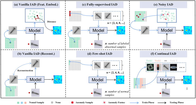
Figure 1: Illustration of the IM-IAD. The vanilla unsupervised IAD methods can be divided into two categories, namely feature embedding-based and reconstruction-based methods. (a) Feature embedding-based methods find the difference between the test samples and normal samples at the feature level, while (b) reconstruction-based methods compare the difference between the input image and the reconstructed image to determine whether it is abnormal or not. For fully supervised methods (c), they use limited abnormal samples with annotations to improve the model performance. The few-shot setting (d) uses a limited number of normal samples for training. The noisy setting (e) mixes abnormal samples in the training set and evaluates the robustness of the model. The continual setting (f) trains on each task in turn and evaluates how much the model forgets past tasks.

II Related Work

This section has reviewed the current IAD methods concluded in Table IM-IAD: Industrial Image Anomaly Detection Benchmark in Manufacturing with five settings that are visualized in Fig. 1 and are defined in Sec. III-A.

Unsupervised IAD. There are two streams methods on unsupervised IAD [52], namely feature embedding-based methods [4, 69, 16, 9], and reconstruction-based methods [88, 97] , [102]. Specifically, feature embedding-based approaches can be divided into four categories, including teacher-student [4], normalizing flow [69], memory bank [16], and one-class classification [76]. The most typical methods are teacher-student models and memory bank-based models. As for teacher-student models, the teacher model extracts the features of normal samples and distils the knowledge to the student model during the training phase. Regarding abnormal images, the features extracted by the teacher network may deviate from those of the student network during the test phase. Thus, the basic rule for finding anomalies is that the teacher-student network has different features. Regarding memory bank-based approaches [16, 50, 43], the models capture the features of normal images and store them in a feature memory bank. During the testing phase, the feature of the test sample queries the memory bank for the feature points of k-nearest neighbourhoods. The test sample is abnormal if the distance between the test feature and the closest feature points of neighbourhoods exceeds a specific threshold. However, both of them heavily depend on the teacher network’s power or the memory bank’s size, which may limit the generalization ability in the real-world industry. Reconstruction-based methods, from those using Autoencoder [6, 97, 11] to Generative Adversarial Network [86, 28], to Transformer [94, 89] and the diffusion model [56, 102], have been employed in recent years. These methods require a significant amount of training time. However, their performance still lags behind feature embedding-based methods, making it challenging to meet the demands of practical industrial production.

Fully supervised IAD. Regarding the setting, the distinction between unsupervised IAD and fully supervised IAD [49, 15, 26] is the use of abnormal images for training. Fully supervised IAD methods [80, 61] focus on efficiently employing a small number of anomalous samples to distinguish the features of abnormalities from those of normal samples. Nevertheless, the performance of some fully supervised IAD approaches is inferior to that of unsupervised methods for identifying anomalies. There is still much room for improvement regarding the use of data from abnormal samples.

Few-shot IAD. Few-shot (including zero-shot) IAD is very promising because it can significantly reduce the demand for data volume. However, it is still in its infancy. GraphCore [84] designs efficient visual isometric invariant features for a few-shot task, which can perform fast training and significantly improve the ability to discriminate anomalies using a few samples. FastRecon [29] stores the features of normal samples to assist image reconstruction during the inference process, enabling the training of the reconstruction network in a few-shot learning scenario. WinCLIP [38] extends the feature comparison approach to zero-shot scenarios. It uses CLIP [64] to extract text features of normal or abnormal descriptions. It compares them with the test image features for anomaly detection. Furthermore, by leveraging diverse multi-modal prior knowledge of foundation models (like Segment Anything [44]) for anomalies, Cao et al. [8] achieve comparable performance on several benchmarks in the zero-shot setting. Recently, AnoVL [25] and AnomalyGPT [31] have achieved new state-of-the-art results in zero-shot scenarios using the understanding capabilities of visual language models, but the size of these models is too large to be deployed in real production lines. Due to the real needs of industrial scenarios, few-shot learning remains a future research focus in anomaly detection.

Noisy IAD. Noisy learning is a classic problem for anomaly detection [63, 12]. However, in the field of IAD, training with noisy data is an inevitable problem in practice. Such noise usually comes from inherent data shifts or human misjudgments. To address this problem, SoftPatch [41] is the first to efficiently denoise data at the patch level in an unsupervised manner. InReaCh [58] strengthens the model’s representation ability by learning the internal relationships within the image. It can achieve results close to SOTA even when trained on artificially corrupted data. By contrast, other methods rarely discuss this situation. The IAD with noisy data needs more research in the future.

Continual IAD. Work integrating continual learning (CL) is growing with the development of anomaly detection. The first CL benchmark for industrial IAD is introduced by Li et al. [51], but their setting ignores the large domain gap of different datasets. LeMO [30] focuses on the problem of continual learning within a class, which, however, neglects the issue of forgetting between classes. To further explore the ability of IAD methods, more efforts should be made in this setting.

III IM-IAD

In this section, we first present the definition of five settings in IM-IAD and then summarize the implementation details of baseline methods, mainstream datasets, evaluation metrics, and hyperparameters. Finally, we point out the importance of studying IM-IAD from a uniform perspective.

III-A Problem Definition

The goal of IAD is that, given a normal or abnormal sample from a target category, the anomaly detection model should predict whether or not the image is anomalous and localize the anomaly region if the prediction result is abnormal. We provide the following five settings.

1. Unsupervised IAD. The training set consists only of $m$ normal samples for each category. The test set contains normal and abnormal samples.

2. Fully supervised IAD. The training set consists of $m$ normal samples and $n$ abnormal samples, where $n\ll m$. In our case, we set $n$ as 10.

3. Few-shot IAD. Given a training set of only $m$ normal samples, where $m\leq 8$, from a certain category. The number of $m$ could be 1, 2, 4, and 8 for the target category, respectively.

4. Noisy IAD. Given a training set of $m$ normal samples and $n$ abnormal samples, $n$ most of 20% of $m+n$. And $n$ abnormal samples are labeled as normal samples in the training dataset.

5. Continual IAD. Given a finite sequence of training dataset $\mathcal{T}_{train}^{total}$ consists of $n$ categories, $\mathcal{T}_{train}^{total}=\left\{\mathcal{T}_{train}^{1},\mathcal{T}_{train}^{2},\cdots,\mathcal{T}_{train}^{n}\right\}$, i.e., $\mathcal{T}_{train}^{total}=\bigcup^{n}_{i=1}\mathcal{T}_{train}^{i}$, where the subsets $\mathcal{T}_{train}^{i}$ consists of normal samples from one certain category $c_{i},i\in n$. The IAD algorithm is trained once for each category dataset $\mathcal{T}_{train}^{i}$ in the CL scenario. During the test, the updated model is evaluated on each category of previous datasets $\mathcal{T}_{test}^{total}$, i.e., $\mathcal{T}_{test}^{total}=\left\{\mathcal{T}_{test}^{1},\mathcal{T}_{test}^{2},\cdots,\mathcal{T}_{test}^{i-1}\right\}$, respectively.

TABLE II: Representative algorithms for IM-IAD. The purple ones indicate our re-implementation methods.

Paradigm			Methods
Vanilla	Feature embeding	Normalizing flow	CS-Flow [70], FastFlow [95], CFlow [32], DifferNet [69]
		Memory bank	PaDiM [21], PatchCore [68], SPADE [16], CFA [46], SOMAD [50], [43]
		Teacher-student	RD4AD [24], STPM [81], [85], [4], [71]
		One-class classification	CutPaste [48], PANDA [66], DROC[76], MOCCA [57],PatchSVDD [91], SE-SVDD [35], [72]
	Reconstruction	External data usage	DREAM [97], DSR [99], MSTUnet[40], DFR [88]
		Internal data usage only	FAVAE [22], NSA [73], RIAD [98], SCADN [86], InTra [62], [6], [34], [54], [17], [87], [23]
Fully supervised			DRA [26], DevNet [61], PRN [100], BGAD [90], SemiREST [49], FCDD [55], SPD [104], CAVGA [80], [15]
Few-shot			RegAD [36], RFS [42], [75]
Noisy label			IGD [12], LOE [63], TrustMAE [78], SROC [18], SRR [93], CPCAD [20]
Continual			DNE [51]

III-B Implementation Datails

III-B1 Baseline Methods

Table II lists 16 IAD algorithms (marked in purple). The criteria for selecting algorithms to be implemented for IM-IAD are that the algorithms should be representative in terms of supervision level (fully supervised and unsupervised), noise-resilient capabilities, the facility of data-efficient adaptation (few shot), and the capacity to overcome catastrophic forgetting. Since most of them achieve state-of-the-art (SOTA) performance on the majority of industrial image datasets, they are referred to as vanilla methods and compared in the IM setting.

III-B2 Datasets

To perform comprehensive ablation studies, we employ seven public datasets in the IM-IAD, including MVTec AD [3, 1], MVTec LOCO-AD [2] MPDD [39], BTAD [59], VisA [104], MTD [37], and DAGM [19]. Table III provides an overview of these datasets, including the number of samples (normal and abnormal samples), the number of classes, the types of anomalies, and the resolution of the image. Pixel-level annotations are available for all datasets. Note that DAGM is a synthetic dataset, MVTec LOCO-AD proposes logical IAD, and VisA proposes multi-instance IAD.

TABLE III: Comparison of datasets in IM-IAD.

	Sample Number		Classes		Image Resolution
Dataset	Normal	Anomaly	Anomaly Type	Object	Min	Max
MVTec AD [3, 1]	4,096	1,258	73	15	700	1,024
MVTec LOCO-AD [2]	2,651	993	89	5	850	1,700
MPDD [39]	1,064	282	5	1	1,024	1,024
BTAD [59]	2,250	580	3	3	600	1,600
MTD [37]	952	392	5	1	113	491
VisA [104]	10,621	1,200	78	12	960	1,562
DAGM [19]	15,000	2,100	10	10	512	512

III-B3 Evaluation Metrics

In terms of structural anomalies, we employ Area Under the Receiver Operating Characteristics (AU-ROC/AUC), Area Under Precision-Recall (AUPR/AP), and PRO [1] to evaluate the abilities of anomaly localization. Regarding logical anomalies, we adopt sPRO [5] to measure the ability of logical defect detection. Additionally, we use the Forgetting Measure (FM) [10] to assess the ability to resist catastrophic forgetting. The relevant formulas are shown in Table IV.

III-B4 Hyperparameters

Table V shows the hyperparameter settings of IM-IAD, including training epochs, batch size, image size, and learning rate, respectively. We share the source codes on the website: https://github.com/M-3LAB/open-iad.

TABLE IV: A summary of metrics used in IM-IAD.

Metric	Better	Formula	Remarks / Usage
Precision (P)	$\uparrow$	$P=TP/(TP+FP)$	True Positive (TP), False Positive (FP)
Recall (R)	$\uparrow$	$R=TP/(TP+FN)$	False Negative (FN)
True Positive Rate (TPR)	$\uparrow$	$TPR=TP/(TP+FN)$	Classification
False Positive Rate (FPR)	$\downarrow$	$FPR=FP/FP+TN)$	True Negative (TN)
Area Under the Receiver Operating Characteristic curve (AU-ROC) [1]	$\uparrow$	$\int_{0}^{1}(TPR)\,{\rm d}(FPR)$	Classification
Area Under Precision-Recall (AU-PR) [1]	$\uparrow$	$\int_{0}^{1}(P)\,{\rm d}(R)$	Localization, Segmentation
Per-Region Overlap (PRO) [1]	$\uparrow$	$PRO=\frac{1}{N}\sum\limits_{i}\sum\limits_{k}\frac{P_{i}\cap C_{i,k}}{C_{i,k}}$	Total ground-truth number (N), Predicted abnormal pixels (P), Defect ground-truth regions (C), Segmentation
Saturated Per-Region Overlap (sPRO) [5]	$\uparrow$	$sPRO(P)=\frac{1}{m}\sum\limits_{i=1}^{m}\min(\frac{A_{i}\cap P}{s_{i}},1)$	Total ground-truth number (m), Predicted abnormal pixels (P), Defect ground-truth regions (A), Corresponding saturation thresholds (s), Segmentation
Forgetting Measure (FM) [10]	$\downarrow$	$FM_{j}^{k}=\max\limits_{l\in\{1,...,k-1\}}\mathbf{T}_{l,j}-\mathbf{T}_{k,j}$	Task (T), Number of tasks (k), Task to be evaluated (j)

TABLE V: Details of experimental settings.

Method	CFA	CSFlow	CutPaste	DNE	DRAEM	FastFlow	FAVAE	IGD	PaDiM	PatchCore	RegAD	RD4AD	SPADE	STPM
Training Epochs	50	240	256	50	700	500	100	256	1	1	50	200	1	100
Batch Size	4	16	32	32	8	32	64	16	32	2	32	8	8	8
Image Size	256	768	224	224	256	256	256	256	256	256	224	256	256	256
Learning Rate	0.001	0.0002	0.0001	0.0001	0.0001	0.001	0.00001	0.0001	\	\	0.0001	0.005	\	0.4

III-C Uniform Perspective

The proposed IM-IAD bridges the connection of different existing settings, as there is no uniform evaluation benchmark.

1) From the perspective of training datasets, the type and number of training samples are the main differences between the five settings shown in Fig. 1. It should be noted that unsupervised IAD algorithms only use normal datasets for training. On the contrary, fully supervised IAD and noisy IAD incorporate a limited quantity of abnormal samples during the training phase. Few-shot IAD employs a limited number of normal samples ($\leq$ 8) for training.

2) From the perspective of applications, IM-IAD are designed to accommodate different scenarios in the real-production line. Since collecting many abnormal samples for training is difficult, unsupervised IAD are designed for a general case via just using normal training samples. Few-shot IAD aims to solve the challenge of cold start in a single assembly line scenario, where normal samples are limited. The goal of continual IAD is to address catastrophic forgetting that occurs when IAD models are integrated into the recycling assembly line. Noisy IAD tries to eliminate the side effects resulting from contaminated training data. Full supervised IAD aims to improve the efficiency of abnormal sample utilization because labelling anomalies is expensive.

III-D Open Challenges

Regarding the setting in IM-IAD, the following is a summary of the challenging issues that need to be investigated.

1) The remaining challenges for fully supervised IAD [26, 49] described in Fig. 1(c) is how to effectively use the guidance of limited abnormal data and a large number of normal samples to detect the anomalies.

2) For the few-shot IAD shown in Fig. 1(d), we aim to detect anomalies in the test set using a small number of normal or abnormal images in the training set [84]. The main obstacles are: i) In a few-shot setting, the training dataset for each category contains only normal samples, meaning there are no annotations at the image or pixel level. ii) Few normal samples of the training set are accessible. In the setting we propose, there are less than eight training samples.

3) We attempt to detect abnormal samples and identify anomalies given a target category for IAD in the presence of noise [41] described in Fig. 1(e). For example, clean training data is assumed to consist exclusively of normal samples. While contaminated training data contains noisy samples incorrectly labelled as normal, i.e., label flipping. Anormal samples are easily mislabeled as normal because the anomalies are too small to identify. The most significant barriers are summarized as follows. i) Each category’s training set contains noisy data that could easily confuse the decision threshold of IAD algorithms. ii) There is a large amount of noisy data. Here, the percentage of anomalous samples in the training set ranges from 5% to 20%. Hence, noisy IAD aims to assess the resilience of current unsupervised IAD methods in the presence of contaminated data.

4) For the continual IAD presented in Fig. 1(f), the greatest challenge is that IAD algorithms may suffer from catastrophic forgetting when they have completed training on the new category dataset. In real-world applications, a single assembly line typically accommodates a substantial amount of workpiece, often containing thousands. Deploying numerous IAD models on a single assembly line is unfeasible due to the high expenses associated with maintenance. Furthermore, a large part of the assembly line process involves recycling. Hence, industrial deployment requires IAD models to overcome catastrophic forgetting.

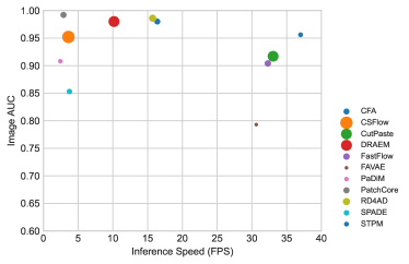
(a) MVTec AD

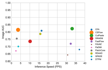
(b) MVTec LOCO-AD

Figure 2: Visualization of vanilla IAD algorithms on Image AUC $\uparrow$, inference time and GPU memory under MVTec AD and LOCO-AD. The Y-axis denotes the performance of the IAD model. The X-axis refers to the inference time taken for each image. The size of the circle denotes the GPU memory consumption of the IAD model during the test phase, where the small one is better.

IV Results and Discussions

This section explores existing algorithms and discusses the critical aspects of the proposed uniform settings. Each part describes experimental facilities, analyzes results, and provides other challenges and future directions.

IV-A Overall Comparisons

Settings. The vanilla methods are presented in Table II. The unsupervised setting is described in Sec. III-A-1.

TABLE VI: Comparison of vanilla IAD algorithms for 7 datasets using 5 metrics. We report sPRO with a 0.05 integration parameter. The best and second-best results are marked in red and blue, respectively.

Dataset	Metric $\uparrow$	CFA	CS-Flow	CutPaste	DRAEM	FastFlow	FAVAE	PaDiM	PatchCore	RD4AD	SPADE	STPM
	Image AUC	0.981	0.952	0.918	0.981	0.905	0.793	0.908	0.992	0.986	0.854	0.924
	Image AP	0.993	0.975	0.965	0.990	0.945	0.913	0.954	0.998	0.995	0.940	0.957
	Pixel AUC	0.971	–	–	0.975	0.955	0.889	0.966	0.994	0.978	0.955	0.954
	Pixel AP	0.538	–	–	0.689	0.398	0.307	0.452	0.561	0.580	0.471	0.518
MVTec AD	Pixel PRO	0.898	–	–	0.921	0.856	0.749	0.913	0.943	0.939	0.895	0.879
	Image AUC	0.814	0.814	0.734	0.798	0.639	0.623	0.780	0.835	0.867	0.687	0.679
	Image AP	0.944	0.942	0.915	0.933	0.866	0.873	0.927	0.948	0.958	0.890	0.891
	Pixel AUC	0.908	–	–	0.942	0.796	0.944	0.987	0.990	0.971	0.971	0.848
	Pixel AP	0.219	–	–	0.209	0.053	0.099	0.149	0.150	0.342	0.261	0.164
MVTec LOCO-AD	Mean sPRO	0.581	–	–	0.426	0.357	0.446	0.521	0.343	0.637	0.520	0.428
	Image AUC	0.923	0.973	0.771	0.941	0.887	0.570	0.706	0.948	0.927	0.784	0.876
	Image AP	0.922	0.968	0.800	0.961	0.881	0.705	0.784	0.970	0.953	0.815	0.914
	Pixel AUC	0.948	–	–	0.918	0.808	0.906	0.955	0.990	0.987	0.982	0.981
	Pixel AP	0.283	–	–	0.288	0.115	0.088	0.155	0.432	0.455	0.342	0.354
MPDD	Pixel PRO	0.832	–	–	0.781	0.498	0.706	0.848	0.939	0.953	0.926	0.939
	Image AUC	0.938	0.936	0.917	0.895	0.919	0.923	0.965	0.947	0.937	0.904	0.918
	Image AP	0.980	0.890	0.953	0.974	0.867	0.986	0.976	0.989	0.985	0.974	0.962
	Pixel AUC	0.959	–	–	0.874	0.965	0.949	0.977	0.978	0.958	0.950	0.937
	Pixel AP	0.517	–	–	0.159	0.379	0.349	0.535	0.520	0.517	0.441	0.401
BTAD	Pixel PRO	0.702	–	–	0.629	0.725	0.713	0.798	0.752	0.723	0.745	0.667
	Image AUC	0.913	0.887	0.830	0.782	0.891	0.795	0.885	0.975	0.884	0.868	0.729
	Image AP	0.959	0.945	0.912	0.885	0.947	0.867	0.944	0.988	0.947	0.928	0.847
	Pixel AUC	0.731	–	–	0.660	0.710	0.735	0.768	0.836	0.693	0.742	0.642
	Pixel AP	0.246	–	–	0.148	0.172	0.120	0.768	0.303	0.218	0.123	0.102
MTD	Pixel PRO	0.528	–	–	0.541	0.568	0.632	0.798	0.686	0.623	0.627	0.478
	Image AUC	0.920	0.744	0.819	0.887	0.822	0.803	0.891	0.951	0.960	0.821	0.833
	Image AP	0.935	0.787	0.848	0.905	0.843	0.843	0.895	0.962	0.965	0.847	0.873
	Pixel AUC	0.843	–	–	0.935	0.882	0.880	0.981	0.988	0.901	0.856	0.834
	Pixel AP	0.268	–	–	0.265	0.156	0.213	0.309	0.401	0.277	0.215	0.169
VisA	Pixel PRO	0.551	–	–	0.724	0.598	0.679	0.859	0.912	0.709	0.659	0.620
	Image AUC	0.948	0.752	0.839	0.908	0.874	0.695	0.940	0.936	0.958	0.714	0.739
	Image AP	0.878	0.781	0.680	0.790	0.699	0.376	0.811	0.826	0.901	0.392	0.498
	Pixel AUC	0.942	–	–	0.868	0.911	0.804	0.961	0.967	0.975	0.880	0.859
	Pixel AP	0.495	–	–	0.306	0.342	0.170	0.492	0.517	0.534	0.133	0.151
DAGM	Pixel PRO	0.870	–	–	0.710	0.799	0.600	0.906	0.893	0.930	0.707	0.668

Discussions. The statistical results of Table VI indicate that there is no universal winner for all datasets. Furthermore, Fig. 2(a) and Fig. 2(b) show that there are no dominant solutions to GPU accuracy, inference speed, and memory. Specifically, Table VI indicates that PatchCore, one of the most advanced memory bank based methods, performs better on MVTec AD than on MVTec LOCO-AD. Because PatchCore architectures specialize in structural anomalies, not logical anomalies, the main differences between MVTec AD and MVTec LOCO-AD are the types of anomalies.

Logical Anomaly Definition. MVTec LOCO-AD consists of structural and logical anomalies. Logical anomalies are not dents or scratches, but are caused by displacement or missing parts. However, MVTec AD only has a structural abnormality. For visualization results, Fig. 3 shows the restrictions of each IAD model to different types of anomalies. For example, the fifth-column images are screw bags, and their defects are logical anomalies. In particular, each box of non-defective screw bags contains exactly one pushpin. However, the defective screw bag contains two pushpins in the upper right corner of the box. The patchcore heatmap cannot accurately represent the anomaly on the right, i.e., whereas RD4AD [24] can precisely identify the logical anomaly on the top right.

Memory Usage and Inference Speed. From Fig. 2, it is clear that there are no dominant IAD methods in terms of accuracy, memory usage and inference time. PatchCore achieves SOTA performance in image AUC, but does not take advantage of memory usage and inference time. In practical scenarios, the use of memory and the speed of inference must be fully taken into account. Therefore, current advanced IAD algorithms cannot meet the requirements of IM.

Image-Level or Pixel-Level Evaluation? Researchers commonly use image-level and pixel-level metrics to evaluate the classification performance of IAD algorithms. In practice, the image-level metric is used to judge whether the whole product is abnormal, while the pixel-level metric indicates anomaly localization performance. To be specific, the pixel-level metric can evaluate the degree of defection, which is strongly associated with the price of products. A lower degree of defects implies a higher price, or vice versa. According to Table VI, specific IAD methods, like PatchCore, perform well on image AUROC but poorly on pixel AP, or vice versa. These two types of metrics signify distinct capabilities of IAD algorithms, and both are very important for IM. Therefore, it is imperative to develop innovative IAD algorithms that exhibit exceptional performance in terms of both image-level metrics and pixel-level metrics.

Challenges. How do we use the types of visual anomalies to select and design unsupervised algorithms effectively? Algorithm selection based on anomalous types is crucial, but there is a lack of research in this area. Since product line specialists can provide information on the type of anomalies, it is appropriate to be aware of the kind of visual anomalies in advance. In other words, knowledge of anomalous types in an unsupervised algorithm can be considered supervision information. Therefore, algorithm designers should consider abnormal types when developing algorithms.

IV-B Role of Global Features in Logical IAD

Settings. We benchmark the vanilla unsupervised IAD algorithms on the MVTec LOCO-AD dataset. In addition, we have re-implemented the baseline logical AD method, GCAD [2].

Discussions. According to Table VII, the baseline method GCAD [2] is superior to all unsupervised IAD methods. The key idea of GCAD [2] is to encode each pixel’s feature descriptor through a bottleneck architecture into a global feature. Existing unsupervised IAD approaches have the disadvantage that their architectures are not optimized to acquire global features.

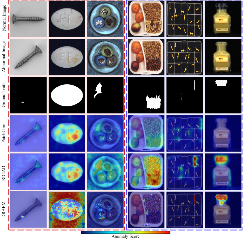
Figure 3: Visualization of the representative vanilla IAD algorithms. The three columns on the left (marked in red) show structural anomalies, while the three columns on the right (marked in blue) show logical anomalies. The first row indicates the training images, where all training images are normal. The second row denotes a test abnormal image and the third row reals the anomalies of the above abnormal image. Lastly, the fourth to sixth row presents the heat map of PatchCore, RD4AD and DRAEM, respectively.

TABLE VII: Benchmark on MVTec LOCO-AD in terms of logical anomalies, structural anomalies and their mean value. The best and second-best results are marked in red and blue, respectively.

	Image AUROC $\uparrow$			Pixel sPRO $\uparrow$
Method	Logical	Structural	Mean	Logical	Strctural	Mean
PatchCore	0.690	0.820	0.755	0.340	0.345	0.343
CFA	0.768	0.851	0.809	0.536	0.625	0.581
SPADE	0.653	0.749	0.701	0.430	0.609	0.520
PaDiM	0.637	0.705	0.671	0.517	0.525	0.521
RD4AD	0.694	0.880	0.787	0.497	0.777	0.637
STPM	0.597	0.763	0.680	0.328	0.529	0.428
CutPaste	0.779	0.867	0.823	–	–	–
CSFlow	0.783	0.847	0.815	–	–	–
FastFlow	0.727	0.712	0.720	0.359	0.356	0.357
DRAEM	0.728	0.744	0.736	0.454	0.398	0.426
FAVAE	0.659	0.628	0.643	0.501	0.392	0.446
GCAD	0.860	0.806	0.833	0.711	0.692	0.701

Challenges. Global feature extraction is crucial to achieving a high detection performance for logical IAD tasks. The statistical results presented in Table VII highlight the significance of global anomaly feature extraction. Recent network architectures such as Transformer [27] and Normalizing Flow [45] focus on long-distance feature extraction, which makes it easier to detect logical anomalies. The results in Table VII show that CSFlow [70], based on Normalizing Flow, achieves the second-best performance regarding logical anomalies, indicating its potential. Additionally, the bottleneck architecture is another feasible approach to capturing global features. As demonstrated by the heat map on the logical anomaly dataset in Fig. 3, the bottleneck design of RD4AD [24] is capable of extracting global features.

IV-C Abnormal Data for Fully Supervised IAD

Settings. We first benchmark fully supervised IAD methods according to the setting in [61, 13, 49]. According to the definition of fully supervised IAD in Sec. III-A-2, we have set the number of abnormal training samples to 10. Here, we make comparisons with PRN [100], BGAD [90], DevNet [61], DRA [26], SemiREST [49], and PatchCore [68].

TABLE VIII: Performance on the fully-supervised setting. The best and second-best results are marked in red and blue, respectively.

Method	Metric $\uparrow$	Bottle	Cable	Capsule	Carpet	Grid	Hazelnut	Leather	Metal_nut	Pill	Screw	Tile	Toothbrush	Transistor	Wood	Zipper	Mean
	Pixel AUC	0.994	0.988	0.985	0.990	0.984	0.997	0.997	0.997	0.995	0.975	0.996	0.996	0.984	0.978	0.988	0.990
	Pixel AP	0.923	0.789	0.622	0.820	0.457	0.938	0.697	0.980	0.913	0.449	0.965	0.781	0.856	0.826	0.776	0.786
PRN	Pixel PRO	0.970	0.972	0.925	0.970	0.959	0.974	0.992	0.958	0.972	0.924	0.982	0.956	0.948	0.959	0.955	0.961
	Pixel AUC	0.993	0.985	0.988	0.996	0.984	0.994	0.998	0.996	0.995	0.993	0.993	0.995	0.979	0.980	0.993	0.992
	Pixel AP	0.871	0.814	0.583	0.832	0.592	0.824	0.755	0.973	0.921	0.553	0.940	0.713	0.823	0.787	0.782	0.784
BGAD	Pixel PRO	0.971	0.977	0.968	0.989	0.987	0.986	0.995	0.968	0.987	0.968	0.979	0.964	0.971	0.968	0.977	0.977
	Pixel AUC	0.939	0.888	0.918	0.972	0.879	0.911	0.942	0.778	0.826	0.603	0.927	0.846	0.560	0.864	0.937	0.853
	Pixel AP	0.515	0.360	0.155	0.457	0.255	0.221	0.081	0.356	0.146	0.014	0.523	0.067	0.064	0.251	0.196	0.244
DevNet	Pixel PRO	0.835	0.809	0.836	0.858	0.798	0.836	0.885	0.769	0.692	0.311	0.789	0.335	0.391	0.754	0.813	0.714
	Pixel AUC	0.913	0.866	0.893	0.982	0.860	0.896	0.938	0.795	0.845	0.540	0.923	0.755	0.791	0.829	0.969	0.853
	Pixel AP	0.412	0.347	0.117	0.523	0.268	0.225	0.056	0.299	0.216	0.050	0.576	0.045	0.110	0.227	0.429	0.260
DRA	Pixel PRO	0.776	0.777	0.791	0.922	0.715	0.869	0.840	0.767	0.770	0.301	0.815	0.561	0.490	0.697	0.910	0.733
	Pixel AUC	0.995	0.992	0.988	0.997	0.994	0.998	0.999	0.999	0.993	0.998	0.997	0.996	0.986	0.992	0.997	0.995
	Pixel AP	0.936	0.895	0.600	0.891	0.664	0.922	0.817	0.991	0.861	0.721	0.969	0.742	0.855	0.887	0.910	0.844
SemiREST	Pixel PRO	0.985	0.959	0.970	0.991	0.970	0.983	0.997	0.982	0.989	0.988	0.989	0.971	0.978	0.979	0.992	0.981
	Pixel AUC	0.988	0.988	0.992	0.992	0.990	0.990	0.994	0.987	0.983	0.996	0.964	0.988	0.961	0.949	0.990	0.994
	Pixel AP	0.768	0.653	0.442	0.627	0.325	0.537	0.456	0.870	0.777	0.354	0.546	0.372	0.610	0.477	0.595	0.561
PatchCore	Pixel PRO	0.957	0.945	0.958	0.949	0.939	0.958	0.974	0.954	0.945	0.964	0.906	0.918	0.906	0.914	0.961	0.943

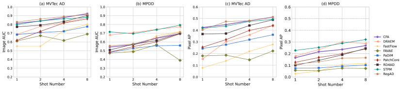
Figure 4: Few-shot IAD Benchmark on MVTec AD and MPDD. The Y-axis refers to the metric value and the X-axis denotes the shot number.

Discussions. Fully supervised IAD algorithms use the distance between test and training samples to predict anomalies. The core idea is that the features of abnormal and normal samples are very different. For example, DevNet [61] proposes using the deviation loss function to enforce the statistical deviation of all anomalies from normal samples. From Table VIII, we can see that the performance of fully supervised IAD methods exceeds that of unsupervised methods (such as PatchCore) in pixel levels by a large margin. It justifies the effectiveness of incorporating an abnormal sample for training.

Challenges. It is essential to improve the efficacy of the abnormal samples for the fully supervised IAD method. Because of the high cost associated with anomaly labels in real applications. On average, each worker spends three hours completing the pixel labels for each image. In subsequent research, researchers have to develop an improved fully supervised IAD algorithm with greater efficiency. The algorithm should reduce the number of abnormal samples for training while maintaining IAD accuracy.

IV-D Rotation Augmentation for Feature-Embedding based Few-Shot IAD

Settings. With respect to the training samples, we choose 1, 2, 4, and 8 to benchmark vanilla IAD methods. Details can be found in the few-shot setting of Sec. III-A-3. In addition, we make a comparison with RegAD [36], which is an advanced method of meta-learning.

Discussions. Fig. 4 shows that CutPaste, STPM, and PatchCore’s performance is comparable to the base model RegAD. Inspired by [60] and [14], we try to improve performance in IM few-shot settings using data augmentation. The statistical results of Table IX indicate that most data augmentation methods are sufficient to improve the few-shot IAD performance. Further, we find that rotation is an optimal augmentation method because most of the real-time industrial image [3, 39] could be transformed into another image by rotation, such as metal_nut and screw.

TABLE IX: Image-level AUC-ROC $\uparrow$ on MVTec AD. The best and second-best results are marked in red and blue, respectively.

Shot	Method	Vanilla	Rotation	Flip	Scale	Translate	ColorJitter	Perspective
	CFA	0.811	0.829	0.811	0.788	0.802	0.814	0.806
	CSFlow	0.708	0.727	0.708	0.742	0.750	0.700	0.713
	CutPaste	0.650	0.701	0.702	0.680	0.679	0.652	0.703
	DRAEM	0.683	0.718	0.715	0.714	0.690	0.687	0.741
	FastFlow	0.527	0.618	0.613	0.694	0.682	0.578	0.600
	FAVAE	0.651	0.560	0.591	0.600	0.581	0.588	0.626
	PaDiM	0.684	0.697	0.683	0.669	0.683	0.681	0.674
	PatchCore	0.788	0.805	0.792	0.788	0.800	0.797	0.789
	RD4AD	0.770	0.805	0.802	0.799	0.823	0.816	0.784
	SPADE	–	–	–	–	–	–	–
1	STPM	0.799	0.841	0.814	0.823	0.843	0.831	0.840
	CFA	0.839	0.860	0.853	0.795	0.825	0.833	0.843
	CSFlow	0.745	0.781	0.773	0.783	0.768	0.754	0.778
	CutPaste	0.697	0.709	0.748	0.659	0.659	0.611	0.726
	DRAEM	0.780	0.765	0.774	0.751	0.771	0.773	0.784
	FastFlow	0.555	0.743	0.674	0.753	0.731	0.628	0.617
	FAVAE	0.667	0.648	0.659	0.595	0.620	0.642	0.631
	PaDiM	0.708	0.734	0.731	0.694	0.716	0.710	0.714
	PatchCore	0.795	0.831	0.805	0.796	0.806	0.793	0.802
	RD4AD	0.798	0.832	0.816	0.835	0.817	0.835	0.820
	SPADE	–	0.737	0.731	0.710	0.734	0.733	0.744
2	STPM	0.840	0.839	0.850	0.848	0.851	0.849	0.838
	CFA	0.879	0.891	0.861	0.818	0.860	0.895	0.883
	CSFlow	0.785	0.841	0.815	0.825	0.810	0.806	0.738
	CutPaste	0.728	0.771	0.714	0.519	0.674	0.621	0.671
	DRAEM	0.820	0.798	0.802	0.819	0.824	0.823	0.826
	FastFlow	0.693	0.741	0.745	0.790	0.782	0.723	0.734
	FAVAE	0.655	0.626	0.669	0.605	0.639	0.670	0.623
	PaDiM	0.722	0.734	0.723	0.689	0.720	0.727	0.716
	PatchCore	0.844	0.872	0.826	0.844	0.848	0.852	0.847
	RD4AD	0.838	0.897	0.871	0.866	0.876	0.872	0.861
	SPADE	–	0.764	0.739	0.749	0.758	0.757	0.759
4	STPM	0.864	0.869	0.865	0.876	0.875	0.868	0.885
	CFA	0.923	0.913	0.888	0.875	0.920	0.919	0.924
	CSFlow	0.856	0.900	0.863	0.900	0.893	0.892	0.861
	CutPaste	0.705	0.808	0.857	0.473	0.694	0.607	0.673
	DRAEM	0.872	0.892	0.905	0.892	0.900	0.904	0.919
	FastFlow	0.828	0.809	0.793	0.843	0.826	0.809	0.810
	FAVAE	0.701	0.651	0.670	0.619	0.611	0.680	0.668
	PaDiM	0.776	0.810	0.739	0.734	0.761	0.779	0.771
	PatchCore	0.891	0.916	0.876	0.889	0.898	0.883	0.891
	RD4AD	0.903	0.933	0.911	0.917	0.921	0.912	0.916
	SPADE	0.781	0.794	0.770	0.783	0.791	0.788	0.787
8	STPM	0.865	0.896	0.870	0.910	0.914	0.912	0.904

Challenges. Synthesis of abnormal samples is essential but difficult. Previously, researchers focused on developing data augmentation methods for normal images. However, little effort is made to synthesize abnormal samples. Because of the fault-free production line in industrial environments, collecting large quantities of abnormal samples is very difficult. In the future, more attention should be paid to abnormal synthesizing methods, such as CutPaste [48] and DRAEM [97].

IV-E Importance Re-weighting for Noisy IAD

Settings. Using the noise setting introduced in Sec. III-A-4, we create a noisy label training dataset by injecting a variety of abnormal samples from the original test set. Specifically, we borrowed the settings from SoftPatch [41]. The abnormal sample accounts for mainly 20% of all training data (called noise ratio). The noise ratio is 5% to 20% and its step size is 5%. Due to the limited size of the test category, we selected a training sample of up to 75% of the abnormal sample of the test dataset. At the training stage, the labels observed in all training datasets are normal. During the test phase, abnormal samples are no longer evaluated. In the noise settings, we benchmark the vanilla and noisy IAD baseline method, IGD [12].

TABLE X: Image AUC $\uparrow$ of Noisy IAD methods on MVTec AD and MPDD under various noise ratios. The best and second-best results are marked in red and blue, respectively.

Dataset	MVTec AD				MPDD
Method	0.05	0.1	0.15	0.2	0.05	0.1	0.15	0.2
CFA	0.969	0.962	0.949	0.946	0.894	0.808	0.839	0.782
CS-Flow	0.939	0.894	0.904	0.874	0.773	0.789	0.861	0.727
CutPaste	0.864	0.900	0.851	0.907	0.773	0.671	0.653	0.683
DRAEM	0.954	0.912	0.869	0.897	0.810	0.760	0.726	0.693
FastFlow	0.885	0.867	0.854	0.855	0.836	0.725	0.725	0.691
FAVAE	0.768	0.801	0.798	0.814	0.536	0.476	0.482	0.525
IGD	0.805	0.801	0.782	0.790	0.797	0.786	0.789	0.756
PaDiM	0.890	0.907	0.899	0.906	0.675	0.580	0.626	0.608
PatchCore	0.990	0.986	0.975	0.980	0.857	0.790	0.782	0.763
RD4AD	0.989	0.984	0.975	0.983	0.909	0.837	0.826	0.824
SPADE	0.854	0.861	0.855	0.859	0.784	0.728	0.737	0.719
STPM	0.909	0.877	0.892	0.915	0.862	0.830	0.848	0.809

Discussions. Based on the statistical findings presented in Table X, it has been discovered that feature embedding-based methods are more effective than IGD when dealing with limited noise levels ($\leq$ 0.15). In order to identify the cause, we have conducted a thorough investigation into the representative feature-embedding based method, PatchCore [68]. During the training phase, the objective is to establish a memory bank that stores neighborhood-aware features from all normal samples. The algorithm used to construct the feature memory is detailed in Algorithm 1.

Input : ImageNet pretrained $\phi$, all normal samples $\mathcal{X}_{N}$ patch feature extractor $\mathcal{P}$, memory size target $l$, random linear projection $\psi$.

Output : Patch-level augmented memory bank $\mathcal{M}$.

1 $\mathcal{M}\leftarrow\left\{\right\}$;

2 for $x_{i}\in\mathcal{X_{N}}$ do

3       $\mathcal{M}\leftarrow\mathcal{M}\cup\mathcal{P}(\phi(x_{i}))$;

4      

5 end for

6$\mathcal{M}_{C}\leftarrow\left\{\right\}$ // Apply coreset sampling for memory bank

7 for $i\in\left[0,\cdots,l-1\right]$ do

8       $m_{i}\leftarrow\underset{m\in\mathcal{M}-\mathcal{M_{C}}}{\operatorname*{arg\,max}}\underset{n\in\mathcal{M_{C}}}{\min}\left\|\psi(m)-\psi(n)\right\|_{2}$;

9       $\mathcal{M_{C}}\leftarrow\mathcal{M_{C}}\cup\left\{m_{i}\right\}$;

10      

11 end for

$\mathcal{M}\leftarrow\mathcal{M_{C}}$.

Algorithm 1 PatchCore Pipeline

TABLE XI: Performance in terms of FM on the continual setting. The best and second-best results are marked in red and blue, respectively.

Dataset	MVTec AD					MPDD
	Image		Pixel			Image		Pixel
Method	AUC$\uparrow$ / FM$\downarrow$	AP$\uparrow$ / FM$\downarrow$	AUC$\uparrow$ / FM$\downarrow$	AP$\uparrow$ / FM$\downarrow$	PRO$\uparrow$ / FM$\downarrow$	AUC$\uparrow$ / FM$\downarrow$	AP$\uparrow$ / FM$\downarrow$	AUC$\uparrow$ / FM$\downarrow$	AP$\uparrow$ / FM$\downarrow$	PRO$\uparrow$ / FM$\downarrow$
PatchCore	0.919 / 0.003	0.971 / 0.001	0.944 / 0.002	0.481 / 0.005	0.847 / 0.001	0.786 / 0.015	0.851 / 0.021	0.963 / 0	0.358 / 0.0004	0.838 / 0.0001
CFA	0.623 / 0.361	0.813 / 0.181	0.753 / 0.217	0.176 / 0.359	0.535 / 0.363	0.506 / 0.415	0.609 / 0.307	0.818 / 0.131	0.116 / 0.164	0.557 / 0.300
SPADE	0.571 / 0.284	0.781 / 0.159	0.746 / 0.208	0.151 / 0.319	0.570 / 0.324	0.412 / 0.396	0.576 / 0.259	0.912 / 0.069	0.139 / 0.202	0.732 / 0.193
PaDiM	0.545 / 0.368	0.767 / 0.192	0.697 / 0.269	0.086 / 0.366	0.441 / 0.472	0.461 / 0.262	0.593 / 0.195	0.841 / 0.116	0.053 / 0.106	0.529 / 0.332
RD4AD	0.596 / 0.392	0.800 / 0.194	0.753 / 0.222	0.143 / 0.425	0.531 / 0.401	0.646 / 0.344	0.833 / 0.162	0.684 / 0.300	0.158 / 0.407	0.532 / 0.414
STPM	0.576 / 0.324	0.786 / 0.163	0.625 / 0.277	0.109 / 0.352	0.322 / 0.446	0.499 / 0.339	0.617 / 0.267	0.328 / 0.648	0.099 / 0.217	0.217 / 0.701
CutPaste	0.312 / 0.509	0.650 / 0.270	–	–	–	0.665 / 0.045	0.724 / 0.061	–	–	–
CSFlow	0.538 / 0.426	0.762 / 0.224	–	–	–	0.632 / 0.343	0.692 / 0.290	–	–	–
FastFlow	0.512 / 0.279	0.713 / 0.154	0.519 / 0.380	0.004 / 0.214	0.152 / 0.562	0.542 / 0.272	0.643 / 0.173	0.269 / 0.506	0.015 / 0.071	0.061 / 0.448
FAVAE	0.547 / 0.101	0.772 / 0.055	0.673 / 0.107	0.082 / 0.082	0.390 / 0.157	0.581 / 0.183	0.792 / 0.099	0.636 / 0.197	0.098 / 0.168	0.365 / 0.267
DNE	0.537 / 0.299	0.533 / 0.293	–	–	–	0.413 / 0.394	0.362 / 0.428	–	–	–

TABLE XII: Image AUROC $\uparrow$ of PatchCore under different noise ratios and neighbourhood numbers. The best and second-best results are marked in red and blue, respectively.

	Neighbour Number
Noise Ratio	1 (No Re-weighting)	2	3	6	9
0.05	0.990	0.988	0.990	0.987	0.990
0.1	0.986	0.989	0.986	0.984	0.983
0.15	0.975	0.983	0.979	0.986	0.984
0.2	0.980	0.982	0.976	0.986	0.982

TABLE XIII: Benchmark of the representative vanilla IAD algorithms in IM-IAD setting, including few-shot, noisy label, continual learning. The best and second-best results are marked in red and blue, respectively.

Dataset		MVTec AD					MPDD
Metric	Method	Vanilla	Noisy-0.15	Few-shot-8	Continual	Mean	Vanilla	Noisy-0.15	Few-shot-8	Continual	Mean
Image AUC $\uparrow$	CFA	0.981	0.949	0.923	0.623	0.869	0.923	0.839	0.694	0.506	0.740
	CSFlow	0.952	0.904	0.845	0.539	0.810	0.973	0.861	0.741	0.633	0.802
	CutPaste	0.918	0.851	0.705	0.312	0.696	0.771	0.653	0.577	0.665	0.667
	DRAEM	0.981	0.869	0.883	0.595	0.832	0.941	0.726	0.773	0.440	0.720
	FastFlow	0.905	0.854	0.801	0.512	0.768	0.887	0.725	0.719	0.543	0.718
	FAVAE	0.793	0.798	0.690	0.547	0.707	0.570	0.482	0.390	0.582	0.506
	PaDiM	0.908	0.899	0.776	0.545	0.782	0.706	0.626	0.560	0.461	0.588
	PatchCore	0.992	0.975	0.864	0.919	0.938	0.948	0.782	0.694	0.787	0.803
	RD4AD	0.986	0.975	0.903	0.596	0.865	0.927	0.826	0.699	0.646	0.775
	SPADE	0.854	0.855	0.781	0.571	0.765	0.784	0.737	0.594	0.412	0.632
	STPM	0.924	0.892	0.880	0.576	0.818	0.876	0.848	0.792	0.499	0.754
Pixel AP $\uparrow$	CFA	0.538	0.394	0.513	0.177	0.406	0.283	0.212	0.269	0.117	0.220
	CSFlow	–	–	–	–	–	–	–	–	–	–
	CutPaste	–	–	–	–	–	–	–	–	–	–
	DRAEM	0.689	0.337	0.442	0.098	0.391	0.288	0.174	0.286	0.131	0.220
	FastFlow	0.398	0.313	0.279	0.044	0.259	0.115	0.055	0.116	0.015	0.075
	FAVAE	0.307	0.319	0.223	0.083	0.233	0.088	0.080	0.073	0.099	0.085
	PaDiM	0.452	0.454	0.362	0.086	0.339	0.155	0.136	0.102	0.053	0.112
	PatchCore	0.561	0.500	0.440	0.481	0.496	0.432	0.254	0.240	0.358	0.321
	RD4AD	0.580	0.532	0.490	0.143	0.436	0.455	0.374	0.245	0.158	0.308
	SPADE	0.471	0.410	0.405	0.151	0.359	0.342	0.309	0.261	0.140	0.263
	STPM	0.518	0.465	0.494	0.110	0.354	0.354	0.309	0.321	0.100	0.271

By default, WideResNet-50 [96] is set as a feature extraction model. Coreset sampling [74] for memory banks aims to balance the size of memory banks with IAD performance. In inference, the test image will be predicted as an anomaly if at least one patch is anomalous, and pixel-level anomaly segmentation will be computed via the score of each patch feature. In particular, with the normal patch feature bank $\mathcal{M}$, the image-level anomaly score $s$ for the test image $x^{test}$ is computed by the maximum score $s^{*}$ between the test image’s patch feature $\mathcal{P}(x^{test})$ and its nearest neighbor $m^{*}$ in $\mathcal{M}$:

$$m^{*}=\underset{m^{test}\in\mathcal{P}(x^{test})}{\operatorname*{arg\,max}}\underset{m\in\mathcal{M}}{\operatorname*{arg\,min}}\left\|m^{test}-m\right\|_{2},$$ (1)

$$s^{*}=\left\|m^{test}-m^{*}\right\|_{2}.$$ (2)

To enhance model robustness, PatchCore employs the importance re-weighting [53] to tune the anomaly score $s$.

$$s=\left(1-\frac{\mathrm{exp}\left\|m^{test,*}-m^{*}\right\|_{2}}{\sum_{m\in\mathcal{N}_{b}(m^{*})}\mathrm{exp}\left\|m^{test,*}-m^{*}\right\|_{2}}\right)\cdot s^{*},$$ (3)

where $\mathcal{N}_{b}(m^{*})$ denotes $b$ nearest patch-features in $\mathcal{M}$ for test patch-feature $m^{*}$. Furthermore, we conducted ablation studies to verify the effect of re-weighting. The statistical result of Table XII shows that re-weighting improves the resilience of IAD algorithms when the noise ratio is larger than 10%.

Challenges. The selection of samples is essential to improve IAD’s robustness. Sample selection has excellent potential in the future, as it can be seamlessly integrated with current IAD methods. For example, Song et al. [77] create a discriminative network to distinguish true-labeled cases from noisy training data, i.e., one for sample selection and the other for anomalous detection.

IV-F Memory Bank-based Methods for Continual IAD

Settings. We benchmark the vanilla methods and the continual baseline IAD method, DNE [51] according to the continual setting in Sec. III-A-5.

Discussions. Table XI indicates that memory bank-based methods provide satisfactory performance to overcome the catastrophic forgetting issue among all unsupervised IAD, even though these methods are not explicitly proposed for continual IAD settings. The main idea is that the replay method is perfectly appropriate for memory-based IAD algorithms. Memory bank-based methods can easily add new memory to reduce forgetting when learning new tasks. Ideally, the memory bank should work for the test mechanism. During the test, the memory bank-based method can easily combine the nearest-mean classifier to locate the nearest memory when the test sample is provided.

Challenges. In the continual IAD setting, limiting the size of the memory database and minimizing interference from previous tasks is of utmost importance. When learning new tasks, simply adding more memory significantly slows down the inference time and increases storage usage. For a fixed storage need, we suggest using the storage sampling [67] to limit the number of instances that can be stored. Furthermore, the memory of the new task may overlap with the memory of the previous task, causing IAD performance to decrease. Consequently, the main challenge is to design a new constraint optimization loss function to avoid task interference.

IV-G Uniform View on IM-IAD

Settings. We benchmark vanilla algorithms in a uniform setting, including few-shot, noisy, and continual settings, which are described in Sec. III-A.

Discussions. Table XIII shows that PatchCore achieves the SOTA result in IM-IAD. However, as shown in Fig. 2, PatchCore is inferior to other IAD algorithms regarding GPU memory usage and inference time, making its use challenging in real scenarios. Furthermore, maintaining the size of the memory bank is a critical issue for realistic deployment if the number of object classes exceeds 100. Therefore, to bridge the gap between academic research and industry, there are still opportunities for IAD algorithms.

Challenges. Multi-objective neural architecture search (NAS) is a considerably promising direction for IAD in finding the optimal trade-off architecture. If the IAD model can be applied in practice, many objectives need to be satisfied, like fast speed of inference, low memory usage, and continual learning ability. Because the memory capacity of edge devices used in production lines is heavily restricted. Moreover, most IAD methods cannot predict the arrival of new test samples instantly when test samples are sequentially streamed on the product line.

V Conclusion

We introduce IM-IAD in this paper, thus far the most complete industrial manufacturing-based IAD benchmark with 19 algorithms, 7 datasets, and 5 settings. We have gained insights into the importance of partial labels for fully supervised learning, the influence of noise ratio in noisy settings, the design principles for continual learning, and the important role of global features for logical anomalies. On top of these, we present several intriguing future lines for industrial IAD.

Acknowledgments

This work is supported by the National Natural Science Foundation of China (Grant NO. 62122035 and 62206122).

Guoyang Xie received the B.Sc. degree from the University of Electronic Science and Technology of China in 2013, the MPhil. degree from the Hong Kong University of Science and Technology in in 2015 and the Ph.D. degree at the University of Surrey, Guildford, United Kingdom in 2023. He is presently an Algorithm Manager in CATL, Ningde, China. Prior to that, he was the Principle Perception Algorithm Engineer in Baidu and GAC, respectively. His research interests include AI for manufacturing and medical imaging, industrial image anomaly detection, robot learning and data synthesis. He has published more than 14 papers in peer-reviewed top-tier conferences (NeurIPS, ICLR, ACM MM, CVPR) and journals (ACM Computing Survey, TCYB, Neurocomputing, Complex & Intelligent System). He has also served as the reviewer for ICML, NeurIPS, ICLR, AAAI, ACM MM, TEVC, TNNLS, TSMC, TETCI.

Jinbao Wang was born in Hebei on 12 Nov. 1989 and received a PhD degree from the University of Chinese Academy of Sciences (UCAS) in 2019. He currently is an Assistant Professor at the National Engineering Laboratory for Big Data System Computing Technology, Shenzhen University, Shenzhen, China. His main research involves computer vision and machine learning, with a long-term focus on image anomaly detection, image generation, and fast retrieval.

Jiaqi Liu received his BS degree from Dalian University of Technology in 2019. He is pursuing the MS degree from Southern University of Science and Technology under the supervision of Professor Feng Zheng. His research interest focuses on image anomaly detection.

Jiayi Lyu was born in Ningxia, China, in 1999. She graduated from Capital Normal University, Beijing, China, and received the bachelor’s degree in July 2021. She is currently pursuing the Ph.D. degree in computer applied technology with the School of Engineering Science, University of Chinese Academy of Sciences, Beijing. Her research interests include image processing and computer graphics.

Yong Liu received the B.S. degree in software engineering from North China Electric Power University, Beijing, China, in 2015, and the M.S. degrees in computer science from the Institute of Computing Technology (ICT), Chinese Academy of Science (CAS), Beijing, China, in 2018. His interests include computer vision, pattern recognition, and machine learning.

Chengjie Wang received the B.S. degree in computer science from Shanghai Jiao Tong University, China, in 2011, and double M.S. degrees in computer science from Shanghai Jiao Tong University, China and Weseda University, Japan, in 2014. He is currently the Research Director of Tencent YouTu Lab. His research interests include computer vision and machine learning. He has published more than 100 papers on major Computer Vision and Artificial Intelligence Conferences such as CVPR, ICCV, ECCV, AAAI, IJCAI and NeurIPS, and holds over 100 patents in these areas.

Feng Zheng received the Ph.D. degree from The University of Sheffield, Sheffield, U.K., in 2017. He is currently an Assistant Professor with the Department of Computer Science and Engineering, Southern University of Science and Technology, Shenzhen, China. His research interests include machine learning, computer vision, and human-computer interaction.

Yaochu Jin (Fellow, IEEE) received the B.Sc., M.Sc., and Ph.D. degrees from Zhejiang University, Hangzhou, China, in 1988, 1991, and 1996, respectively, and the Dr.-Ing. degree from Ruhr University Bochum, Germany, in 2001. He is presently Chair Professor of AI, Head of the Trustworthy and General AI Lab, School of Engineering, Westlake University, Hangzhou, China. Prior to that, he was Alexander von Humboldt Professor for Artificial Intelligence endowed by the German Federal Ministry of Education and Research, with the Faculty of Technology, Bielefeld University, Germany from 2021 to 2023, and Surrey Distinguished Chair, Professor in Computational Intelligence, Department of Computer Science, University of Surrey, Guildford, U.K. from 2010 to 2021. He was also “Finland Distinguished Professor” with University of Jyväskylä, Finland, and “Changjiang Distinguished Visiting Professor” with the Northeastern University, China from 2015 to 2017. His main research interests include evolutionary optimization, evolutionary machine learning, trustworthy AI, and evolutionary developmental AI. Prof Jin is the President of the IEEE Computational Intelligence Society and Editor-in-Chief of Complex & Intelligent Systems. He was named by the Web of Science as “a Highly Cited Researcher” from 2019 to 2023 consecutively. He is a Member of Academia Europaea.

References

- [1] Paul Bergmann, Kilian Batzner, Michael Fauser, David Sattlegger, and Carsten Steger. The mvtec anomaly detection dataset: a comprehensive real-world dataset for unsupervised anomaly detection. International Journal of Computer Vision, 129(4):1038–1059, 2021.
- [2] Paul Bergmann, Kilian Batzner, Michael Fauser, David Sattlegger, and Carsten Steger. Beyond dents and scratches: Logical constraints in unsupervised anomaly detection and localization. International Journal of Computer Vision, 130(4):947–969, 2022.
- [3] Paul Bergmann, Michael Fauser, David Sattlegger, and Carsten Steger. Mvtec ad — a comprehensive real-world dataset for unsupervised anomaly detection. 2019 IEEE/CVF Conference on Computer Vision and Pattern Recognition (CVPR), pages 9584–9592, 2019.
- [4] Paul Bergmann, Michael Fauser, David Sattlegger, and Carsten Steger. Uninformed students: Student-teacher anomaly detection with discriminative latent embeddings. In Proceedings of the IEEE/CVF Conference on Computer Vision and Pattern Recognition, pages 4183–4192, 2020.
- [5] Paul Bergmann, Xin Jin, David Sattlegger, and Carsten Steger. The mvtec 3d-ad dataset for unsupervised 3d anomaly detection and localization. arXiv preprint arXiv:2112.09045, 2021.
- [6] Paul Bergmann, Sindy Löwe, Michael Fauser, David Sattlegger, and Carsten Steger. Improving unsupervised defect segmentation by applying structural similarity to autoencoders. arXiv preprint arXiv:1807.02011, 2018.
- [7] Luca Bonfiglioli, Marco Toschi, Davide Silvestri, Nicola Fioraio, and Daniele De Gregorio. The eyecandies dataset for unsupervised multimodal anomaly detection and localization. In Asian Conference on Computer Vision, 2022.
- [8] Yunkang Cao, Xiaohao Xu, Chen Sun, Yuqi Cheng, Zongwei Du, Liang Gao, and Weiming Shen. Segment any anomaly without training via hybrid prompt regularization. arXiv preprint arXiv:2305.10724, 2023.
- [9] Yunkang Cao, Xiaohao Xu, Chen Sun, Liang Gao, and Weiming Shen. Bias: Incorporating biased knowledge to boost unsupervised image anomaly localization. IEEE Transactions on Systems, Man, and Cybernetics: Systems, pages 1–12, 2024.
- [10] Arslan Chaudhry, Puneet Kumar Dokania, Thalaiyasingam Ajanthan, and Philip H. S. Torr. Riemannian walk for incremental learning: Understanding forgetting and intransigence. ArXiv, abs/1801.10112, 2018.
- [11] Ruitao Chen, Guoyang Xie, Jiaqi Liu, Jinbao Wang, Ziqi Luo, Jinfan Wang, and Feng Zheng. Easynet: An easy network for 3d industrial anomaly detection. In Proceedings of the 31st ACM International Conference on Multimedia, pages 7038–7046, 2023.
- [12] Yuanhong Chen, Yu Tian, Guansong Pang, and G. Carneiro. Deep one-class classification via interpolated gaussian descriptor. In AAAI, 2022.
- [13] Yuanhong Chen, Yu Tian, Guansong Pang, and Gustavo Carneiro. Deep one-class classification via interpolated gaussian descriptor. Proceedings of the AAAI Conference on Artificial Intelligence, 36(1):383–392, 2022.
- [14] Z. Chen, Yanwei Fu, Kaiyu Chen, and Yu-Gang Jiang. Image block augmentation for one-shot learning. In AAAI Conference on Artificial Intelligence, 2019.
- [15] Wen-Hsuan Chu and Kris M Kitani. Neural batch sampling with reinforcement learning for semi-supervised anomaly detection. In European conference on computer vision, pages 751–766. Springer, 2020.
- [16] Niv Cohen and Yedid Hoshen. Sub-image anomaly detection with deep pyramid correspondences. arXiv preprint arXiv:2005.02357, 2020.
- [17] Anne-Sophie Collin and Christophe De Vleeschouwer. Improved anomaly detection by training an autoencoder with skip connections on images corrupted with stain-shaped noise. In 2020 25th International Conference on Pattern Recognition (ICPR), pages 7915–7922. IEEE, 2021.
- [18] Antoine Cordier, Benjamin Missaoui, and Pierre Gutierrez. Data refinement for fully unsupervised visual inspection using pre-trained networks. arXiv preprint arXiv:2202.12759, 2022.
- [19] German chapter of the IAPR (International Association for Pattern Recognition)) DAGM (Deutsche Arbeitsgemeinschaft für Mustererkennung e.V. and the GNSS (German Chapter of the European Neural Network Society). Dagm dataset. http://www.thisisurl/, 2000.
- [20] Puck de Haan and Sindy Löwe. Contrastive predictive coding for anomaly detection. arXiv preprint arXiv:2107.07820, 2021.
- [21] Thomas Defard, Aleksandr Setkov, Angelique Loesch, and Romaric Audigier. Padim: a patch distribution modeling framework for anomaly detection and localization. In International Conference on Pattern Recognition, pages 475–489. Springer, 2021.
- [22] David Dehaene and Pierre Eline. Anomaly localization by modeling perceptual features. ArXiv, abs/2008.05369, 2020.
- [23] David Dehaene, Oriel Frigo, Sébastien Combrexelle, and Pierre Eline. Iterative energy-based projection on a normal data manifold for anomaly localization. In International Conference on Learning Representations, 2019.
- [24] Hanqiu Deng and Xingyu Li. Anomaly detection via reverse distillation from one-class embedding. ArXiv, abs/2201.10703, 2022.
- [25] Hanqiu Deng, Zhaoxiang Zhang, Jinan Bao, and Xingyu Li. Anovl: Adapting vision-language models for unified zero-shot anomaly localization. arXiv preprint arXiv:2308.15939, 2023.
- [26] Choubo Ding, Guansong Pang, and Chunhua Shen. Catching both gray and black swans: Open-set supervised anomaly detection. In Proceedings of the IEEE/CVF Conference on Computer Vision and Pattern Recognition, pages 7388–7398, 2022.
- [27] Alexey Dosovitskiy, Lucas Beyer, Alexander Kolesnikov, Dirk Weissenborn, Xiaohua Zhai, Thomas Unterthiner, Mostafa Dehghani, Matthias Minderer, Georg Heigold, Sylvain Gelly, Jakob Uszkoreit, and Neil Houlsby. An image is worth 16x16 words: Transformers for image recognition at scale. ArXiv, abs/2010.11929, 2020.
- [28] Yuxuan Duan, Yan Hong, Li Niu, and Liqing Zhang. Few-shot defect image generation via defect-aware feature manipulation. In Proceedings of the AAAI Conference on Artificial Intelligence, volume 37, pages 571–578, 2023.
- [29] Zheng Fang, Xiaoyang Wang, Haocheng Li, Jiejie Liu, Qiugui Hu, and Jimin Xiao. Fastrecon: Few-shot industrial anomaly detection via fast feature reconstruction. In Proceedings of the IEEE/CVF International Conference on Computer Vision, pages 17481–17490, 2023.
- [30] Han Gao, Huiyuan Luo, Fei Shen, and Zhengtao Zhang. Towards total online unsupervised anomaly detection and localization in industrial vision. arXiv preprint arXiv:2305.15652, 2023.
- [31] Zhaopeng Gu, Bingke Zhu, Guibo Zhu, Yingying Chen, Ming Tang, and Jinqiao Wang. Anomalygpt: Detecting industrial anomalies using large vision-language models. arXiv preprint arXiv:2308.15366, 2023.
- [32] Denis Gudovskiy, Shun Ishizaka, and Kazuki Kozuka. Cflow-ad: Real-time unsupervised anomaly detection with localization via conditional normalizing flows. In Proceedings of the IEEE/CVF Winter Conference on Applications of Computer Vision, pages 98–107, 2022.
- [33] Songqiao Han, Xiyang Hu, Hailiang Huang, Mingqi Jiang, and Yue Zhao. Adbench: Anomaly detection benchmark. ArXiv, abs/2206.09426, 2022.
- [34] Jinlei Hou, Yingying Zhang, Qiaoyong Zhong, Di Xie, Shiliang Pu, and Hong Zhou. Divide-and-assemble: Learning block-wise memory for unsupervised anomaly detection. In Proceedings of the IEEE/CVF International Conference on Computer Vision, pages 8791–8800, 2021.
- [35] Chuanfei Hu, Kai Chen, and Hang Shao. A semantic-enhanced method based on deep svdd for pixel-wise anomaly detection. In 2021 IEEE International Conference on Multimedia and Expo (ICME), pages 1–6. IEEE, 2021.
- [36] Chaoqin Huang, Haoyan Guan, Aofan Jiang, Ya Zhang, Michael Spratling, and Yan-Feng Wang. Registration based few-shot anomaly detection. arXiv preprint arXiv:2207.07361, 2022.
- [37] Yibin Huang, Congying Qiu, and Kui Yuan. Surface defect saliency of magnetic tile. The Visual Computer, 36(1):85–96, 2020.
- [38] Jongheon Jeong, Yang Zou, Taewan Kim, Dongqing Zhang, Avinash Ravichandran, and Onkar Dabeer. Winclip: Zero-/few-shot anomaly classification and segmentation. In Proceedings of the IEEE/CVF Conference on Computer Vision and Pattern Recognition, pages 19606–19616, 2023.
- [39] Stepan Jezek, Martin Jonak, Radim Burget, Pavel Dvorak, and Milos Skotak. Deep learning-based defect detection of metal parts: evaluating current methods in complex conditions. In 2021 13th International Congress on Ultra Modern Telecommunications and Control Systems and Workshops (ICUMT), pages 66–71. IEEE, 2021.
- [40] Jielin Jiang, Jiale Zhu, Muhammad Bilal, Yan Cui, Neeraj Kumar, Ruihan Dou, Feng Su, and Xiaolong Xu. Masked swin transformer unet for industrial anomaly detection. IEEE Transactions on Industrial Informatics, 2022.
- [41] Xi Jiang, Jianlin Liu, Jinbao Wang, Qiang Nie, Kai Wu, Yong Liu, Chengjie Wang, and Feng Zheng. Softpatch: Unsupervised anomaly detection with noisy data. Advances in Neural Information Processing Systems, 35:15433–15445, 2022.
- [42] Ammar Mansoor Kamoona, Amirali Khodadadian Gostar, Alireza Bab-Hadiashar, and Reza Hoseinnezhad. Anomaly detection of defect using energy of point pattern features within random finite set framework. arXiv preprint arXiv:2108.12159, 2021.
- [43] Jin-Hwa Kim, Do-Hyeong Kim, Saehoon Yi, and Taehoon Lee. Semi-orthogonal embedding for efficient unsupervised anomaly segmentation. arXiv preprint arXiv:2105.14737, 2021.
- [44] Alexander Kirillov, Eric Mintun, Nikhila Ravi, Hanzi Mao, Chloe Rolland, Laura Gustafson, Tete Xiao, Spencer Whitehead, Alexander C Berg, Wan-Yen Lo, et al. Segment anything. arXiv preprint arXiv:2304.02643, 2023.
- [45] Ivan Kobyzev, Simon Prince, and Marcus A. Brubaker. Normalizing flows: Introduction and ideas. ArXiv, abs/1908.09257, 2019.
- [46] Sungwook Lee, Seunghyun Lee, and Byung Cheol Song. Cfa: Coupled-hypersphere-based feature adaptation for target-oriented anomaly localization. arXiv preprint arXiv:2206.04325, 2022.
- [47] Chao Li, Jun Li, Yafei Li, Lingmin He, Xiaokang Fu, and Jingjing Chen. Fabric defect detection in textile manufacturing: a survey of the state of the art. Security and Communication Networks, 2021:1–13, 2021.
- [48] Chun-Liang Li, Kihyuk Sohn, Jinsung Yoon, and Tomas Pfister. Cutpaste: Self-supervised learning for anomaly detection and localization. In Proceedings of the IEEE/CVF Conference on Computer Vision and Pattern Recognition, pages 9664–9674, 2021.
- [49] Hanxi Li, Jingqi Wu, Hao Chen, Mingwen Wang, and Chunhua Shen. Efficient anomaly detection with budget annotation using semi-supervised residual transformer. arXiv preprint arXiv:2306.03492, 2023.
- [50] Ning Li, Kaitao Jiang, Zhiheng Ma, Xing Wei, Xiaopeng Hong, and Yihong Gong. Anomaly detection via self-organizing map. In 2021 IEEE International Conference on Image Processing (ICIP), pages 974–978. IEEE, 2021.
- [51] Wujin Li, Jiawei Zhan, Jinbao Wang, Bizhong Xia, Bin-Bin Gao, Jun Liu, Chengjie Wang, and Feng Zheng. Towards continual adaptation in industrial anomaly detection. In Proceedings of the 30th ACM International Conference on Multimedia, pages 2871–2880, 2022.
- [52] Jiaqi Liu, Guoyang Xie, Jingbao Wang, Shangnian Li, Chengjie Wang, Feng Zheng, and Yaochu Jin. Deep industrial image anomaly detection: A survey. arXiv preprint arXiv:2301.11514, 2, 2023.
- [53] Tongliang Liu and Dacheng Tao. Classification with noisy labels by importance reweighting. IEEE Transactions on Pattern Analysis and Machine Intelligence, 38:447–461, 2014.
- [54] Wenqian Liu, Runze Li, Meng Zheng, Srikrishna Karanam, Ziyan Wu, Bir Bhanu, Richard J Radke, and Octavia Camps. Towards visually explaining variational autoencoders. In Proceedings of the IEEE/CVF Conference on Computer Vision and Pattern Recognition, pages 8642–8651, 2020.
- [55] Philipp Liznerski, Lukas Ruff, Robert A Vandermeulen, Billy Joe Franks, Marius Kloft, and Klaus Robert Muller. Explainable deep one-class classification. In International Conference on Learning Representations, 2020.
- [56] Fanbin Lu, Xufeng Yao, Chi-Wing Fu, and Jiaya Jia. Removing anomalies as noises for industrial defect localization. In Proceedings of the IEEE/CVF International Conference on Computer Vision, pages 16166–16175, 2023.
- [57] Fabio Valerio Massoli, Fabrizio Falchi, Alperen Kantarci, Şeymanur Akti, Hazim Kemal Ekenel, and Giuseppe Amato. Mocca: Multilayer one-class classification for anomaly detection. IEEE Transactions on Neural Networks and Learning Systems, 2021.
- [58] Declan McIntosh and Alexandra Branzan Albu. Inter-realization channels: Unsupervised anomaly detection beyond one-class classification. In Proceedings of the IEEE/CVF International Conference on Computer Vision, pages 6285–6295, 2023.
- [59] Pankaj Mishra, Riccardo Verk, Daniele Fornasier, Claudio Piciarelli, and Gian Luca Foresti. Vt-adl: A vision transformer network for image anomaly detection and localization. In 2021 IEEE 30th International Symposium on Industrial Electronics (ISIE), pages 01–06. IEEE, 2021.
- [60] Renkun Ni, Micah Goldblum, Amr Sharaf, Kezhi Kong, and Tom Goldstein. Data augmentation for meta-learning. In International Conference on Machine Learning, 2020.
- [61] Guansong Pang, Choubo Ding, Chunhua Shen, and Anton van den Hengel. Explainable deep few-shot anomaly detection with deviation networks. arXiv preprint arXiv:2108.00462, 2021.
- [62] Jonathan Pirnay and Keng Chai. Inpainting transformer for anomaly detection. In International Conference on Image Analysis and Processing, pages 394–406. Springer, 2022.
- [63] Chen Qiu, Aodong Li, Marius Kloft, Maja Rudolph, and Stephan Mandt. Latent outlier exposure for anomaly detection with contaminated data. arXiv preprint arXiv:2202.08088, 2022.
- [64] Alec Radford, Jong Wook Kim, Chris Hallacy, Aditya Ramesh, Gabriel Goh, Sandhini Agarwal, Girish Sastry, Amanda Askell, Pamela Mishkin, Jack Clark, et al. Learning transferable visual models from natural language supervision. In International conference on machine learning, pages 8748–8763. PMLR, 2021.
- [65] Punit Rathore, Dheeraj Kumar, James C. Bezdek, Sutharshan Rajasegarar, and Marimuthu Swami Palaniswami. Visual structural assessment and anomaly detection for high-velocity data streams. IEEE Transactions on Cybernetics, 51:5979–5992, 2020.
- [66] Tal Reiss, Niv Cohen, Liron Bergman, and Yedid Hoshen. Panda: Adapting pretrained features for anomaly detection and segmentation. 2021 IEEE/CVF Conference on Computer Vision and Pattern Recognition (CVPR), pages 2805–2813, 2021.
- [67] David Rolnick, Arun Ahuja, Jonathan Schwarz, Timothy P. Lillicrap, and Greg Wayne. Experience replay for continual learning. In NeurIPS, 2019.
- [68] Karsten Roth, Latha Pemula, Joaquin Zepeda, Bernhard Schölkopf, Thomas Brox, and Peter Gehler. Towards total recall in industrial anomaly detection. In Proceedings of the IEEE/CVF Conference on Computer Vision and Pattern Recognition, pages 14318–14328, 2022.
- [69] Marco Rudolph, Bastian Wandt, and Bodo Rosenhahn. Same same but differnet: Semi-supervised defect detection with normalizing flows. In Proceedings of the IEEE/CVF winter conference on applications of computer vision, pages 1907–1916, 2021.
- [70] Marco Rudolph, Tom Wehrbein, Bodo Rosenhahn, and Bastian Wandt. Fully convolutional cross-scale-flows for image-based defect detection. In Proceedings of the IEEE/CVF Winter Conference on Applications of Computer Vision, pages 1088–1097, 2022.
- [71] Mohammadreza Salehi, Niousha Sadjadi, Soroosh Baselizadeh, Mohammad H Rohban, and Hamid R Rabiee. Multiresolution knowledge distillation for anomaly detection. In Proceedings of the IEEE/CVF conference on computer vision and pattern recognition, pages 14902–14912, 2021.
- [72] Daniel Sauter, Anna Schmitz, Fulya Dikici, Hermann Baumgartl, and Ricardo Buettner. Defect detection of metal nuts applying convolutional neural networks. In 2021 IEEE 45th Annual Computers, Software, and Applications Conference (COMPSAC), pages 248–257. IEEE, 2021.
- [73] Hannah M Schlüter, Jeremy Tan, Benjamin Hou, and Bernhard Kainz. Self-supervised out-of-distribution detection and localization with natural synthetic anomalies (nsa). arXiv preprint arXiv:2109.15222, 2021.
- [74] Ozan Sener and Silvio Savarese. Active learning for convolutional neural networks: A core-set approach. arXiv: Machine Learning, 2018.
- [75] Shelly Sheynin, Sagie Benaim, and Lior Wolf. A hierarchical transformation-discriminating generative model for few shot anomaly detection. In Proceedings of the IEEE/CVF International Conference on Computer Vision, pages 8495–8504, 2021.
- [76] Kihyuk Sohn, Chun-Liang Li, Jinsung Yoon, Minho Jin, and Tomas Pfister. Learning and evaluating representations for deep one-class classification. In International Conference on Learning Representations, 2020.
- [77] Hwanjun Song, Minseok Kim, and Jae-Gil Lee. Selfie: Refurbishing unclean samples for robust deep learning. In International Conference on Machine Learning, 2019.
- [78] Daniel Stanley Tan, Yi-Chun Chen, Trista Pei-Chun Chen, and Wei-Chao Chen. Trustmae: A noise-resilient defect classification framework using memory-augmented auto-encoders with trust regions. In Proceedings of the IEEE/CVF winter conference on applications of computer vision, pages 276–285, 2021.
- [79] Colin SC Tsang, Henry YT Ngan, and Grantham KH Pang. Fabric inspection based on the elo rating method. Pattern Recognition, 51:378–394, 2016.
- [80] Shashanka Venkataramanan, Kuan-Chuan Peng, Rajat Vikram Singh, and Abhijit Mahalanobis. Attention guided anomaly localization in images. In European Conference on Computer Vision, pages 485–503. Springer, 2020.
- [81] Guodong Wang, Shumin Han, Errui Ding, and Di Huang. Student-teacher feature pyramid matching for anomaly detection. In BMVC, 2021.
- [82] Hengli Wang, Rui Fan, Yuxiang Sun, and Ming Liu. Dynamic fusion module evolves drivable area and road anomaly detection: A benchmark and algorithms. IEEE transactions on cybernetics, 52(10):10750–10760, 2021.
- [83] Min Wang, Donghua Zhou, and Maoyin Chen. Hybrid variable monitoring mixture model for anomaly detection in industrial processes. IEEE transactions on cybernetics, PP, 2022.
- [84] Guoyang Xie, Jinbao Wang, Jiaqi Liu, Yaochu Jin, and Feng Zheng. Pushing the limits of fewshot anomaly detection in industry vision: Graphcore. In The Eleventh International Conference on Learning Representations, 2023.
- [85] Shinji Yamada and Kazuhiro Hotta. Reconstruction student with attention for student-teacher pyramid matching. arXiv preprint arXiv:2111.15376, 2021.
- [86] Xudong Yan, Huaidong Zhang, Xuemiao Xu, Xiaowei Hu, and Pheng-Ann Heng. Learning semantic context from normal samples for unsupervised anomaly detection. In Proceedings of the AAAI Conference on Artificial Intelligence, volume 35, pages 3110–3118, 2021.
- [87] Yi Yan, Deming Wang, Guangliang Zhou, and Qijun Chen. Unsupervised anomaly segmentation via multilevel image reconstruction and adaptive attention-level transition. IEEE Transactions on Instrumentation and Measurement, 70:1–12, 2021.
- [88] Jie Yang, Yong Shi, and Zhiquan Qi. Dfr: Deep feature reconstruction for unsupervised anomaly segmentation. arXiv preprint arXiv:2012.07122, 2020.
- [89] Xincheng Yao, Ruoqi Li, Zefeng Qian, Yan Luo, and Chongyang Zhang. Focus the discrepancy: Intra-and inter-correlation learning for image anomaly detection. In Proceedings of the IEEE/CVF International Conference on Computer Vision, pages 6803–6813, 2023.
- [90] Xincheng Yao, Ruoqi Li, Jing Zhang, Jun Sun, and Chongyang Zhang. Explicit boundary guided semi-push-pull contrastive learning for supervised anomaly detection. In Proceedings of the IEEE/CVF Conference on Computer Vision and Pattern Recognition, pages 24490–24499, 2023.
- [91] Jihun Yi and Sungroh Yoon. Patch svdd: Patch-level svdd for anomaly detection and segmentation. In Proceedings of the Asian Conference on Computer Vision, 2020.
- [92] Yong-Ho Yoo, Ue-Hwan Kim, and Jong hwan Kim. Convolutional recurrent reconstructive network for spatiotemporal anomaly detection in solder paste inspection. IEEE Transactions on Cybernetics, 52:4688–4700, 2019.
- [93] Jinsung Yoon, Kihyuk Sohn, Chun-Liang Li, Sercan O Arik, Chen-Yu Lee, and Tomas Pfister. Self-supervise, refine, repeat: Improving unsupervised anomaly detection. 2021.
- [94] Zhiyuan You, Lei Cui, Yujun Shen, Kai Yang, Xin Lu, Yu Zheng, and Xinyi Le. A unified model for multi-class anomaly detection. Advances in Neural Information Processing Systems, 35:4571–4584, 2022.
- [95] Jiawei Yu, Ye Zheng, Xiang Wang, Wei Li, Yushuang Wu, Rui Zhao, and Liwei Wu. Fastflow: Unsupervised anomaly detection and localization via 2d normalizing flows. arXiv preprint arXiv:2111.07677, 2021.
- [96] Sergey Zagoruyko and Nikos Komodakis. Wide residual networks. In Procedings of the British Machine Vision Conference 2016. British Machine Vision Association, 2016.
- [97] Vitjan Zavrtanik, Matej Kristan, and Danijel Skočaj. Draem-a discriminatively trained reconstruction embedding for surface anomaly detection. In Proceedings of the IEEE/CVF International Conference on Computer Vision, pages 8330–8339, 2021.
- [98] Vitjan Zavrtanik, Matej Kristan, and Danijel Skočaj. Reconstruction by inpainting for visual anomaly detection. Pattern Recognition, 112:107706, 2021.
- [99] Vitjan Zavrtanik, Matej Kristan, and Danijel Skočaj. Dsr–a dual subspace re-projection network for surface anomaly detection. arXiv preprint arXiv:2208.01521, 2022.
- [100] Hui Zhang, Zuxuan Wu, Zheng Wang, Zhineng Chen, and Yu-Gang Jiang. Prototypical residual networks for anomaly detection and localization. In Proceedings of the IEEE/CVF Conference on Computer Vision and Pattern Recognition, pages 16281–16291, 2023.
- [101] Jian Zhang, Ge Yang, Miaoju Ban, and Runwei Ding. Pku-goodsad: A supermarket goods dataset for unsupervised anomaly detection and segmentation. arXiv preprint arXiv:2307.04956, 2023.
- [102] Xinyi Zhang, Naiqi Li, Jiawei Li, Tao Dai, Yong Jiang, and Shu-Tao Xia. Unsupervised surface anomaly detection with diffusion probabilistic model. In Proceedings of the IEEE/CVF International Conference on Computer Vision, pages 6782–6791, 2023.
- [103] Ye Zheng, Xiang Wang, Yu-Hang Qi, Wei Li, and Liwei Wu. Benchmarking unsupervised anomaly detection and localization. ArXiv, abs/2205.14852, 2022.
- [104] Yang Zou, Jongheon Jeong, Latha Pemula, Dongqing Zhang, and Onkar Dabeer. Spot-the-difference self-supervised pre-training for anomaly detection and segmentation. arXiv preprint arXiv:2207.14315, 2022.