Learning Choice Functions via Pareto-Embeddings

Abstract

We consider the problem of learning to choose from a given set of objects, where each object is represented by a feature vector. Traditional approaches in choice modelling are mainly based on learning a latent, real-valued utility function, thereby inducing a linear order on choice alternatives. While this approach is suitable for discrete (top-1) choices, it is not straightforward how to use it for subset choices. Instead of mapping choice alternatives to the real number line, we propose to embed them into a higher-dimensional utility space, in which we identify choice sets with Pareto-optimal points. To this end, we propose a learning algorithm that minimizes a differentiable loss function suitable for this task. We demonstrate the feasibility of learning a Pareto-embedding on a suite of benchmark datasets.

Keywords Choice function  $\cdot$ Pareto-embedding  $\cdot$ Generalized utility

1 Introduction

The quest for understanding and modeling human decision making has a long history in various scientific disciplines, including economics and psychology [4]. Starting with the seminal work by Arrow [1], choice functions have been analyzed as a key concept of a formal theory of choice. In simple terms, a decision maker is confronted with a (possibly varying) set of alternatives and the choices made are observed. The ultimate goal is to explain and predict the choice behavior.

In machine learning, the task of “learning to choose” is part of the broader field of preference learning, which attracted increased attention in recent years [5]. The task for a learner is to observe choices from multiple sets of objects, and to produce a function which maps from candidate sets to choice sets. An important special case is the setting in which the decision maker only chooses one object from each given set, which is known as discrete choice. A popular strategy to tackle the learning problem is to posit that the choice probabilities depend on an underlying real-valued utility function of the decision maker. Under this assumption, learning can be accomplished by identiying the parameters of such a function. The more general problem of predicting choices in the form of subsets of objects has been considered only very recently [2, 11]. Extending the approach based on utility functions toward this setting turns out to be non-trivial. Either one faces combinatorial problems calculating the probabilities for many subsets [2], or has to resort to thresholding techniques [11].

We propose to solve this problem by embedding the objects in a higher-dimensional utility space, in which subset choices are naturally identified by Pareto-optimal points (Section 3). To learn a suitable embedding function, we devise a differentiable loss function tailored to this task. We then utilize the loss function as part of a deep learning pipeline to investigate the feasibility of learning such a Pareto-embedding (Section 4).

2 Modeling Choice

We proceed from a reference set of objects (choice alternatives) $\mathcal{X}\subset\mathbb{R}^{d}$, which, for ease of exposition, is assumed to be finite. Each $\boldsymbol{x}\in\mathcal{X}$ is represented as a vector of real-valued features $(x_{1},\dots,x_{d})$. We call a finite subset of objects $Q\subseteq\mathcal{X}$ a choice task and allow the size $|Q|\in\mathbb{N}$ to vary across tasks. For each choice task $Q=\{\boldsymbol{x}_{1},\ldots,\boldsymbol{x}_{m}\}$, we assume that a preference is expressed in terms of a choice set $C\subseteq Q$. A useful representation of a choice set is in terms of a binary vector $\boldsymbol{c}\in\{0,1\}^{m}$, where $c_{i}=1$ if $\boldsymbol{x}_{i}\in C$ and $c_{i}=0$ if $\boldsymbol{x}_{i}\not\in C$.

One of the first approaches to explaining choices was to assume that a decision maker can assign a (latent) utility to each of the choice alternatives. Formally, we represent such a utility function as a function $\mathcal{X}\to\mathbb{R}$ from the space of objects to the real numbers. Based on these utilities, a rational decision maker will always pick the alternative with the highest utility, i. e., the top-1 object. To explain variability in choices, noise can be added to the utilities, which results in what is called a random utility model [12, 8, 7].

At first glance, it may appear that this approach can easily be generalized to modeling subset choices: Instead of only selecting the top-1 object, one could consider to select the top-$k$ objects, where $1\leq k\leq|Q|$. One major drawback of this approach is that the subset size is predetermined to be $k$, so it is not possible to produce subsets of varying size. Another possibility is to specify a threshold for the utilities, and to include all objects with a utility higher than the threshold in the choice set [11]. While this allows for the prediction of subsets of arbitrary size, the decision of whether to include an object in the choice set is now completely independent of all the other objects.

As we shall see in the next section, there is a natural way to define subset choices, if we embed the objects in a higher-dimensional utility space.

3 Pareto-Embeddings

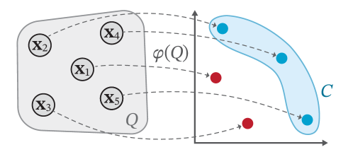
Figure 1: A Pareto-embedding $\varphi(\cdot)$ maps a given set of objects $Q$ into a higher-dimensional space $\mathcal{Z}$. The Pareto-optimal points in this space we define to be the choice set $C$.

The basic idea of a Pareto-embedding is illustrated in Fig. 1. On the left side, we depict the original set of objects in the object space $\mathcal{X}$. The function $\varphi\colon\mathcal{X}\to\mathcal{Z}$ maps each point into a new embedding space $\mathcal{Z}\subseteq\mathbb{R}^{d^{\prime}}$. This space can be thought of as a higher-dimensional utility space, i. e., each dimension corresponds to the utility on a certain aspect or criterion. As we can see, the choice set $C$ forms what is called a Pareto-set in this new space, i. e., the set of points that are not dominated by any other point.

More formally, let $Q=\{\boldsymbol{x}_{1},\dots,\boldsymbol{x}_{m}\}\subseteq\mathcal{X}$ be the original set of objects and $Z=\varphi(Q)=\{\boldsymbol{z}_{1},\dots,\boldsymbol{z}_{m}\}=\{\varphi(\boldsymbol{x}_{1}),\dots,\varphi(\boldsymbol{x}_{m})\}$ the corresponding points in the embedding space. A point $\boldsymbol{z}_{i}$ in the embedding space is dominated by another point $\boldsymbol{z}_{j}$ if $z_{i,k}\leq z_{j,k}$ for all $k\in[d^{\prime}]$ and $z_{i,k}<z_{j,k}$ for at least one such $k$. Then, a point $\boldsymbol{z}_{i}$ is called Pareto-optimal (with respect to $Z$), if it is not dominated by any other point $\boldsymbol{z}_{j}\in Z$, $1\leq j\neq i\leq m$. We denote by $P_{\varphi}(Q)\subseteq Q$ the subset of points that are Pareto-optimal in $Q$ under the mapping $\varphi$, i.e., the points $\boldsymbol{x}_{i}\in Q$ such that $\varphi(\boldsymbol{x}_{i})$ not dominated by any point in $\{\varphi(\boldsymbol{x}_{1}),\dots,\varphi(\boldsymbol{x}_{m})\}$.

It is interesting to note that the traditional one-dimensional utility always imposes a total order relation on the available objects, whereas the Pareto-embedding generalizes this to a partial order. Therefore, richer preference structures with multiple layers of incomparability can be modeled.

Given a set of observed choices $\mathcal{D}=\{(Q_{n},C_{n})\}_{n=1}^{N}$ as training data, where $Q_{n}\subseteq\mathcal{X}$ is a choice task and $C_{n}\subseteq Q_{n}$ the subset of objects selected, we are interested in learning a Pareto-embedding $\varphi$ coherent with this data in the sense that $C_{n}\approx P_{\varphi}(Q_{n})$ for all $n\in[N]$. Obviously, a function of that kind can then also be used for predictive purposes, i.e., to predict the choice for a new choice task. To induce $\varphi$ from $\mathcal{D}$, we devise a general-purpose loss function, which can be used with any end-to-end trainable model, and hence should be differentiable almost everywhere.

The loss function we propose consists of several components, which we introduce step by step. Consider a choice $C$ in a choice task $Q$, and denote by $\boldsymbol{c}\in\{0,1\}^{|Q|}$ the vector encoding of $C$, i.e., $c_{i}=1$ if $\boldsymbol{x}_{i}\in C$ and $c_{i}=0$ otherwise. In order to accomplish $C=P_{\varphi}(Q)$, the first constraint to be fulfilled by $\varphi$ is to ensure that each point $\boldsymbol{x}_{j}\in C$ will have an image in the embedding space which is Pareto-optimal in $Z$.

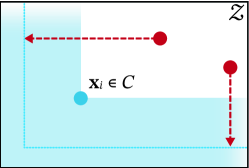
(a) $L_{\text{PO}}$

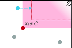
(b) $L_{\text{DOM}}$

Figure 2: Visualization of the effect of the loss terms $L_{\text{PO}}$ and $L_{\text{DOM}}$ in $\mathcal{Z}$ space.

Consider Fig. 2a, where the point in blue depicts the image $\boldsymbol{z}_{j}=(z_{j,1},\ldots,z_{j,d^{\prime}})$ of $\boldsymbol{x}_{j}$. The loss needs to penalize all points dominating $\boldsymbol{z}_{j}$ (shown in red). Formally, the first part of the loss function is defined as follows:

$$L_{\text{PO}}(Z,\boldsymbol{c}) =\sum_{1\leq i\neq j\leq|Z|}\max\Bigl{(}0,c_{j}\cdot\min_{1\leq k\leq d^{\prime}}(1+z_{i,k}-z_{j,k})\Bigr{)}$$ (1)

We project the points towards the blue region using the minimum term and penalize them in proportion from their distance to the boundary. Note that, to enforce a margin effect, we already penalize non-dominating points close to the boundary. This corresponds to using a hinge loss upper bound on the 0/1-binary loss, which is 1 if $\boldsymbol{z}_{i}$ dominates $\boldsymbol{z}_{j}$ and 0 otherwise.

Similarly, we define a loss that penalizes the embedding of a point $\boldsymbol{x}_{i}\in Q\setminus C$ so that $\boldsymbol{x}_{i}$ is not dominated:

$$L_{\text{DOM}}(Z,\boldsymbol{c}) =\sum_{i=1}^{\lvert Z\rvert}(1-c_{i})\min_{j\neq i}\biggl{(}\,\sum_{k=1}^{d^{\prime}}\max\big{(}0,1+z_{i,k}-z_{j,k}\big{)}\biggr{)}$$ (2)

The minimum selects the point which is closest to dominating $\boldsymbol{z}_{i}$, while the inner sum penalizes all dimensions in which this point is not yet better than $\boldsymbol{z}_{i}$.

With these two terms, we can ensure that if the loss is 0, we have a valid Pareto-embedding of the points. Furthermore, we add two more terms that are useful. To preserve as much of the original structure present in the object space $\mathcal{X}$, we use multidimensional scaling (MDS) [9]. It ensures that objects close to each other in the object space $\mathcal{X}$ will also be close in the embedding space $\mathcal{Z}$. In addition, all the losses so far are shift-invariant in the embedding space. To make the solution identifiable, we regularize the mapped points towards 0 using an $L_{2}$ loss. We define the complete Pareto-embedding loss as a convex combination

$$L(Q,Z,\boldsymbol{c}) =\alpha_{1}L_{\text{PO}}(Z,\boldsymbol{c})+\alpha_{2}L_{\text{DOM}}(Z,\boldsymbol{c})+\alpha_{3}L_{\text{MDS}}(Q,Z)+\alpha_{4}\sum_{i=1}^{\lvert Z\rvert}\lVert\boldsymbol{z}_{i}\rVert_{2}$$

with weights $\alpha_{1},\alpha_{2},\alpha_{3},\alpha_{4}\geq 0$ such that $\alpha_{1}+\alpha_{2}+\alpha_{3}+\alpha_{4}=1$. These weights can be treated as hyperparameters of the learning algorithm. Given a space $\Phi$ of embedding functions, this algorithm seeks to find a minimizer

$$\varphi^{*}\in\operatorname*{argmin}_{\varphi\in\Phi}\sum_{n=1}^{N}L\big{(}Q_{n},P_{\varphi}(Q_{n}),\boldsymbol{c}_{n}\big{)}$$

of the overall loss on the training data $\mathcal{D}$.

4 Empirical Evaluation

As for the space of embedding functions, any model class amenable to training by gradient descent can in principle be used. Here, as a proof of concept, we use a simple fully connected multi-layer perceptron as a learner. The architecture is depicted in Fig. 3.

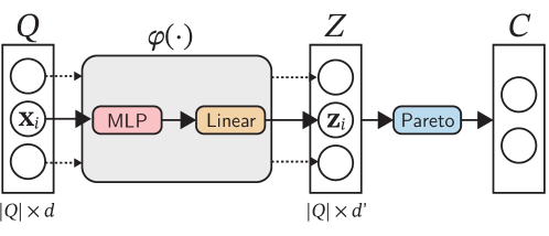
Figure 3: Architecture of our approach. Each object is passed through a (deep) multi-layer perceptron followed by a linear output layer to produce the embedding. The Pareto-optimal points are selected to obtain a prediction $C$.

We take each object $\boldsymbol{x}_{i}$ for $1\leq i\leq|Q|$ of the task $Q$ and pass it through the (deep) multi-layer perceptron. Rectified linear units are used here as the nonlinearities. Batch normalization [6] is applied after each layer to speed up and stabilize training. In the final layer, we pass the output of the multi-layer perceptron through a linear layer with $d^{\prime}$ outputs. After the same network (using weight sharing) was applied to all objects in $Q$, we end up with the transformed set $Z$. To obtain the final prediction, we take the set $Z$ and compute the corresponding Pareto-set. The network can be trained using standard backpropagation of the loss.

To ascertain the feasibility of learning a Pareto-embedding from data, we evaluate our approach on a suite of benchmark problems from the field of multi-criteria optimization. We use the well-known DTLZ test suite by Deb et al. [3] and the ZDT test suite by Zitzler et al. [13], containing datasets of varying difficulty. Adding a simple two-dimensional two parabola (TP) dataset, we end up with 14 benchmark problems in total. We generate $40\,960$ object sets of size 10 with 6 features each for every problem. Exceptions are the TP dataset with only 2 features and the ZDT5 dataset, which has 35 binary features by definition. For the DTLZ problems, we set the dimensionality of the underlying objective space to 5.

We evaluate our approach on every problem by 5 repetitions of a Monte Carlo cross validation with a 90/10% split into training and test data. The remaining instances are split into $\mathrm{1}\mathrm{/}\mathrm{9}$ validation instances and $\mathrm{8}\mathrm{/}\mathrm{9}$ training instances. We use the validation set to jointly optimize the hyperparameters of the learner, which are (a) the loss weights $\alpha_{1},\alpha_{2},\alpha_{3},\alpha_{4}$, (b) the maximum learning rate of the cyclical learning rate scheduler, and (c) the number of hidden units and layers, using $60$ iterations of Bayesian optimization. The neural network was trained for 500 epochs. The number of embedding dimensions $d^{\prime}$ we set to 2, since this allows us to move from a total order (only one utility dimension) to a partial order.

Finally, we need a suitable metric to compare the ground truth subsets to the predicted ones. Since the shape of the Pareto-sets has an impact on how many points end up in the chosen subset, we have varying levels of positives across the datasets. Therefore, we choose a metric that is unbiased with respect to the prevalence of positives and well-suited for problems with class imbalance, called the A-mean [10], the arithmetic mean of the true positive and true negative rate.

The results are shown in Fig. 4.

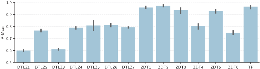
Figure 4: Results of the empirical evaluation. The bars show the average performance in terms of A-mean across the 5 outer splits. The sticks show the estimated standard deviation.

For five of the problems, the embedding approach is able to achieve an average A-mean of over $90\text{\,}\frac{\mathrm{\char 37\relax}}{}$, indicating that for these problems we often identify the choice set correctly. This is important, as it shows that the loss function is able to steer the model parameters towards a valid Pareto-embedding. For comparison, a random selection in which each object is included in the choice set with a fixed probability (independently of the others) achieves an average A-mean of $50\text{\,}\frac{\mathrm{\char 37\relax}}{}$. Thus, it is apparent that our learner is performing better than random guessing on all datasets. We also did an ablation experiment, where we removed the MDS term from the loss function and repeated the complete training procedure (including optimization of all the other hyperparameters). This resulted in a significant decrease in performance, showing that the MDS term is not only useful to preserve distances, but adds a helpful inductive bias.

5 Conclusion and Outlook

We proposed a novel way to tackle the problem of learning choice functions. Viewing it as an embedding problem and transforming the given objects into a utility space of more than one dimension, subset choice are naturally identified by the criterion of Pareto-optimality. To learn an embedding from a given set of observed choices as training data, we developed a suitable loss function that penalizes violations of the Pareto condition. Encouraged by the promising first results on benchmark problems, we are now looking forward to a more extensive empirical evaluation and applications to real-world choice problems.

expansion=sloppy

References

- Arrow [1951] Arrow, K.J.: Social Choice and Individual Values. John Wiley & Sons (1951)
- Benson et al. [2018] Benson, A.R., Kumar, R., Tomkins, A.: A Discrete Choice Model for Subset Selection. In: Proceedings of the Eleventh ACM International Conference on Web Search and Data Mining. pp. 37–45. WSDM ’18, ACM (2018)
- Deb et al. [2005] Deb, K., Thiele, L., Laumanns, M., Zitzler, E.: Scalable Test Problems for Evolutionary Multiobjective Optimization, pp. 105–145. Springer London, London (2005)
- Domshlak et al. [2011] Domshlak, C., Hüllermeier, E., Kaci, S., Prade, H.: Preferences in AI: An overview. Artificial Intelligence 175(7–8), 1037–1052 (2011)
- Fürnkranz and Hüllermeier [2010] Fürnkranz, J., Hüllermeier, E. (eds.): Preference Learning. Springer (2010)
- Ioffe and Szegedy [2015] Ioffe, S., Szegedy, C.: Batch normalization: Accelerating deep network training by reducing internal covariate shift. In: Proceedings of the 32nd International Conference on Machine Learning, ICML 2015, Lille, France, 6-11 July 2015. JMLR Workshop and Conference Proceedings, vol. 37, pp. 448–456. JMLR.org (2015)
- Luce [1959] Luce, R.D.: Individual Choice Behavior. John Wiley (1959)
- Marschak [1959] Marschak, J.: Binary Choice Constraints on Random Utility Indicators. Tech. Rep. 74, Cowles Foundation for Research in Economics, Yale University (1959)
- Mead [1992] Mead, A.: Review of the development of multidimensional scaling methods. Journal of the Royal Statistical Society. Series D (The Statistician) 41(1), 27–39 (1992)
- Menon et al. [2013] Menon, A., Narasimhan, H., Agarwal, S., Chawla, S.: On the Statistical Consistency of Algorithms for Binary Classification under Class Imbalance. In: Proceedings of the 30th International Conference on Machine Learning. Proceedings of Machine Learning Research, vol. 28, pp. 603–611. PMLR, Atlanta, Georgia, USA (17–19 Jun 2013)
- Pfannschmidt et al. [2019] Pfannschmidt, K., Gupta, P., Hüllermeier, E.: Learning Choice Functions: Concepts and Architectures. CoRR abs/1901.10860 (2019)
- Thurstone [1927] Thurstone, L.L.: A law of comparative judgment. Psychological Review 34(4), 273–286 (1927)
- Zitzler et al. [2000] Zitzler, E., Deb, K., Thiele, L.: Comparison of Multiobjective Evolutionary Algorithms: Empirical Results. Evol. Comput. 8(2), 173–195 (Jun 2000)