Intelligent Credit Limit Management in Consumer Loans
Based on Causal Inference
Abstract
Nowadays consumer loan plays an important role in promoting the economic growth, and credit cards are the most popular consumer loan. One of the most essential parts in credit cards is the credit limit management. Traditionally, credit limits are adjusted based on limited heuristic strategies, which are developed by experienced professionals. In this paper, we present a data-driven approach to manage the credit limit intelligently. Firstly, a conditional independence testing is conducted to acquire the data for building models. Based on these testing data, a response model is then built to measure the heterogeneous treatment effect of increasing credit limits (i.e. treatments) for different customers, who are depicted by several control variables (i.e. features). In order to incorporate the diminishing marginal effect, a carefully selected log transformation is introduced to the treatment variable. Moreover, the model’s capability can be further enhanced by applying a non-linear transformation on features via GBDT encoding. Finally, a well-designed metric is proposed to properly measure the performances of compared methods. The experimental results demonstrate the effectiveness of the proposed approach.
1 Introduction
Consumer loan helps people to finance their consumption demand, and nowadays it plays an important role in promoting the economic growth Rona-Tas and Guseva (2018). The most popular consumer loans are credit cards, which enable borrowers to make everyday purchases Hodson et al. (2014). The credit limit (or line) management is one of the most essential parts in the risk management of credit cards. In credit limit management, a maximum loan amount is set for each credit account, according to customer’s credit risk, consumer demand and so on. The total amount of money that customers own to the lender is referred as credit balance. Most lenders are trying to maximize their credit balance, since the balance is the foundation of their revenues. Through better credit limit management, the whole credit limit can be allocated to right places and the total credit balance can be then increased efficiently. For instance, a lender may give the opportunity of increasing the credit limit to a customer whose utilization is already very high as long as the credit risk is low enough. What’s more, improving the credit limit management can also lead to better customer relationships, since more customers’ consumption demands can be satisfied.
When managing the credit limit, there are several factors to take into account, including credit risk, consumer demand, historical balance and current limit etc. In traditional credit limit management, the limit is adjusted by experienced professionals in a heuristic and rule-based way. Although quantitative methods have been already utilized in credit limit management for a long time Rosenberg and Gleit (1994) Gross et al. (2000) Sohn et al. (2014), the whole process heavily relies on manual analyses and interventions, which greatly limits the sophistication of limit adjusting strategies. More specifically, the customers can only be segmented into a few heterogeneous groups, and the decision of limit adjustment is made for each group according to expert experiences. As the requirement of associated expert experiences is high, the traditional approach of managing credit limit is quite expensive. In addition, the development cycle of strategies is too long and the strategies is too simply for the dynamic and complex business environment in consumer loans nowadays.
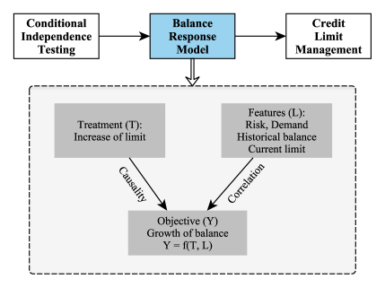
In recent decade, as many data about customers’ behaviors have been collected, a lot of data-driven methods are leveraged to gain deeper insights into business environment, which helps us to make more informed decisions. In this paper, we present a data-driven approach to manage the credit limit in an intelligent way, and the whole framework is illustrated in Figure 1. To determine the increasing amount of credit limit for a particular customer, we need to predict the customer’s response to the limit adjustment. In other words, we need to build a balance response model, which depicts the relationship between the increase of limit (i.e. treatment) and the growth of balance (i.e. objective). Different customers have different balance response curves, and the shape of each curve is determined by the specific factors (i.e. control variables or features) of corresponding customer. Most traditional machine learning methods are based on correlation study. They are incompetent to model the reliable relationship between the treatment and the objective, and thus cannot generalize to counterfactual predictions111The empirical evidence on real-world data will be later illustrated in the experimental section.. Recently, causal inference attracts a lot of attentions from both research and industry communities. A more robust and stable decision-making system can be built if we model causality instead of correlation between the decision and the outcome Hernan and Robins (2010) Imbens and Rubin (2015).
The majority of existing researches on causality focus on modeling with observed data, where treatments are not assigned randomly along control variables but intervened by some unknown confounders. The observational study relies on several assumptions, and it might be hard to validate them in practice, especially for the conditional independence assumption and the common support assumption Peters et al. (2017). On the other hand, although randomized testing is the gold standard for estimating the causal effect, it is costly and even infeasible in most scenarios. To overcome these challenges, we design and conduct a conditional independence testing, where the above two assumptions are perfectly satisfied, to acquire the data for building models. Based on the testing data, a structural outcome regression model is built to measure the heterogeneous treatment effect of increasing credit limits for different customers. The diminishing marginal effect is a common phenomenon in many scenarios and also exists in credit limit management without surprise. We introduce a carefully selected log transformation to the treatment variable to incorporate this prior knowledge. Furthermore, inspired by He et al. (2014), the capability of our structural model can be enhanced by applying a non-linear transformation on features via GBDT encoding. Finally, we propose a proper evaluation metric to measure the performances of compared methods. The experimental results demonstrate the effectiveness of our approach.
The rest of our paper is organized as follows. We briefly review related work in Section 2. We present the setup of testing in Section 3, and how to build and evaluate the balance response model in Section 4. The experimental results and further analyses are presented in Section 5. The conclusions and future plans are given in Section 6.
2 Related Work
The credit card is the most popular type of consumer loan Hodson et al. (2014), and quantitative methods have already been utilized in its risk management for a long time Rosenberg and Gleit (1994) Thomas (2000). One essential part in the risk management of credit cards is credit limit management. Soman and Cheema (2002) argued that consumers use their credit limits as a signal of future potential earnings, and hence the credit limit would positively impact their spend. Gross et al. (2000) and Song (2011) investigated consumers’ responses to the change of credit limits, and the results show that increases in credit limits can effectively raise the credit balance. Inspired by these results, the credit limit can be adjusted by experienced professionals in a simple heuristic and rule-based way. To increase the sophistication of credit limit management, some more advanced approaches have been proposed. Dey (2010) discussed the possibility of using simulation along with action-effect models to set the optimum credit limit for each account. Paul and Biswas (2017) tried to assign credit limit to new customers using Bayesian decision theory and Fuzzy logic. Unfortunately, these works focus on concepts or theoretical studies without empirical results, and thus it is hard to assess their effectiveness in real-world applications. Sohn et al. (2014) developed a strategy to maximize the total net profit by adjusting individual credit limits, and they demonstrated its effectiveness on real-world data from FICO. However, the customers can only be segmented into a few heterogeneous groups, and the whole process heavily relies on manual analyses and interventions.
In recent decade, data-driven methods have been successfully applied to many business applications Jordan and Mitchell (2015), such as credit risk models in consumer loans Khandani et al. (2010) Addo et al. (2018). In order to manage the credit limit in a more sophisticated and intelligent way, the response of each customer to the limit adjustment need to be predicted. Although big data and powerful algorithms can achieve better forecasting performance in many tasks, there are gaps between forecasting and decision making Athey (2017). Traditional machine or deep learning methods, which are based on correlation study, are incompetent to model the causality between the input factors and the target. Recently, causal inference has been widely studied and applied to many domains Hernan and Robins (2010) Pearl (2009) Morgan and Winship (2015) Imbens and Rubin (2015). One important topic in causal inference is to estimate the average treatment effect Jordà and Taylor (2016) Machado et al. (2019). The other equally important topic is to estimate the heterogeneous treatment effect, where Athey and Imbens (2016) and Wager and Athey (2018) are two popular methods under the binary treatment. In this work, we are interested in estimating the heterogeneous treatment effect of increases in the credit limit, which are continuous treatments, for different customers. Moreover, although the common observational study has several drawbacks, they can be readily overcome in practice by conducting a conditional independence testing Peters et al. (2017). To our best knowledge, we are the first to utilize the causal inference to tackle the credit limit management in the real-world scenario.
| Credit rating | Treatment | |||||||
|---|---|---|---|---|---|---|---|---|
| 0 | 5 | 10 | 20 | 30 | 60 | 100 | 150 | |
| Very Good | 20 | 20 | 20 | 20 | 20 | |||
| Good | 20 | 20 | 20 | 20 | 20 | |||
| Fair | 20 | 20 | 20 | 20 | 20 | |||
| Poor | 20 | 20 | 20 | 20 | 20 | |||
3 Testing
We are interested in predicting the potential outcome (i.e. growth of balance) under different treatments (i.e. increases of limit) when keeping everything else constant, and it is referred as counterfactual prediction. For example, we want to know the growth of balance for a customer if we increase her credit limit by 10000, which has not ever been observed in the real-world. Since the counterfactual prediction is beyond the ability of traditional machine learning methods, we turn to causal inference and build a balance response model to estimate the heterogenous treatment effect when increasing the credit limit for a customer. However, a fundamental problem in causal inference is that only one treatment could be conducted for an individual at the same time, which means the data for the counterfactual reasoning are missing Hernan and Robins (2010). Based on the observed data, this problem can be solved in observational study if the bias caused by confounders can be effectively eliminated.
3.1 Observational study
| Demand level | Treatment | |||
|---|---|---|---|---|
| 0 | 100 | 200 | 300 | |
| High | 25 | 25 | 25 | 25 |
In the observed data, treatments were assigned through some unknown strategies. There may be some factors that affect both treatment assignment and outcome, and they are referred as confounders. Thus for observational study, a major challenge is how to eliminate the bias caused by confounders. Under the conditional independence assumption (or unconfoundedness), which assumes all confounders have been observed, several techniques can be exploited to overcome this challenge. A commonly used technique is based on the propensity score Rosenbaum and Rubin (1983), which is the probability that a customer is given a specific treatment :
| (1) |
where denotes the observed features, and denotes the treatment. As long as the propensity score is estimated, the Inverse Probability of Treatment Weighting (IPTW) can be leveraged to balance the distribution of treatments and remove the bias caused by confounders Hirano et al. (2003):
| (2) |
As we can see, the IPTW method also implicitly relies on another assumption that there should exist overlaps among different treatments under the same observed features:
| (3) |
This assumption is also known as common support. Actually, for many other techniques in observational study, such as outcome regression, the above two assumptions are also required, though it might be hard to validate them in practice.
| Demand level | Treatment | |||
|---|---|---|---|---|
| 0 | 50 | 100 | 150 | |
| Low | 25 | 25 | 25 | 25 |
3.2 Conditional independence testing
The randomized testing is the gold standard for causal inference, and the mentioned assumptions can be satisfied naturally Imbens and Rubin (2015). However, randomized testing is costly and even infeasible in most scenarios. For example, we cannot increase the credit limit too much for a customer who has a poor credit rating, because it is very likely to cause a loss. Fortunately, we can conduct a conditional independence testing that satisfies those assumptions as well Peters et al. (2017). In the conditional independence testing, treatments are randomly assigned conditional on specific features , and the dependence between features and treatments is broken down under the given : . Since the confounders are introduced artificially, the conditional independence assumption is obviously satisfied.
When designing the conditional independence testing, it is crucial to choose the proper artificial confounder. In this work, we construct based on the credit rating and the consumer demand. At first, we split the customers into two groups according to their credit rating: prime group and sub-prime group. For the sub-prime group, the customers are further segmented into four subgroups with different credit ratings: very good, good, fair, and poor (as illustrated in Table 1) 222Without loss of generality, all the treatment values have been scaled by a constant to avoid divulging business secrets.. For the prime group, the customers are further segmented into two subgroups with different demand levels: high and low (as illustrated in Table 2 and Table 3). The dummy coding of above six subgroups is set as . What’s more, to meet the common support assumption, we keep a proportion of customers’ credit limits unchanged in each subgroup. As we can see, the increase of credit limit in each subgroup is bounded in a range, which is determined by business rules and will be maintained in productization. For instance, the increases of credit limits are relatively small for the customers with high credit risk, and greater increases of credit limits are assigned to the prime customers with higher demand level.
4 Balance Response Model
Based on the testing data, we build a balance response model to predict the growth of balance under increases in the credit limit for different customers. The model is built within the framework of potential outcome Rubin (2005) Edin (2018).
4.1 Problem formulation
Firstly, let us formally introduce several important conceptions used in our model:
Treatment: Treatment is defined as the increase of credit limit for a customer,
and it is a continuous variable.
Outcome: Outcome is defined as the growth of
credit balance over a period of time,
denotes the potential outcome under the treatment .
For example, if (and ) denotes the monthly average balance
before (and after) increasing the credit limit by , .
Feature: There are plenty of features in real-world productization,
and we select some representative features in this paper without loss of generality.
-
•
Credit risk: the probability of default, the credit rating.
-
•
Consumption: the monthly average spends over the last 3 months and 6 months respectively, the monthly maximum spend over the last 12 months.
-
•
Historical balance: the monthly average balances over the last 3 months and 6 months respectively.
-
•
Current limit: the credit limit before adjustment.
Besides these features, the artificial confounder should also be included in features . Then the outcome regression model is correctly specified, and no more adjustment is required Hernan and Robins (2010).
We aim to build a model to conduct the counterfactual prediction given the features and treatment :
| (4) |
As the treatment is a continuous variable, the local effect around a treatment point can be calculated, and it is referred as heterogeneous marginal effect:
| (5) |
The straightforward linear regression is the most simple choice to model the relationship between , and :
| (6) |
The marginal effect can be directly interpreted by the coefficient :
| (7) |
As we can see, the marginal effect is independence of , which means that customers with different features would have the same marginal causal effect, and it is obviously inconsistent with the actual situation.
4.2 Structural outcome regression
In fact, customers with different features should have different marginal causal effects. If we assume that the outcome is a linear function of the treatment , the relationship between , and can be depicted by a structural outcome regression model:
| (8) |
Note that the simple linear regression is a special case, where and . The heterogeneous marginal effect is computed as follow:
| (9) |
which is determined only by features and independent of the treatment .
Actually, the diminishing marginal effect exists in the credit limit management, which means that the marginal causal effect should decrease along with the increase of treatment . In order to incorporate this prior knowledge, we introduce a log transformation to the treatment as follow:
| (10) |
where is a hyper-parameter. Then the marginal effect is computed as follow:
| (11) |
which indicates that the outcome would increase slower as the treatment increases.
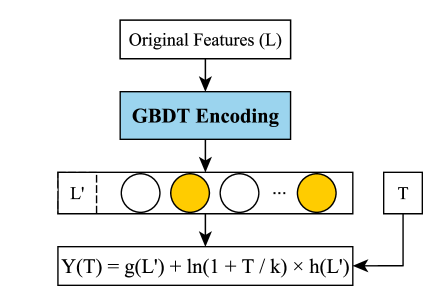
In the traditional outcome regression, and are linear functions of , and their capabilities are limited. Inspired by He et al. (2014), we apply a non-linear transformation to features through a GBDT encoding. Firstly, a GBDT model is built to predict the outcome based on features without the treatment . Then, the original features is transformed into new features via the acquired GBDT model. Finally, is used instead of to build the outcome regression model as follow (also illustrated in Figure 2) :
| (12) |
When training the outcome regression model, the objective is to minimize the Mean Square Error (MSE), and the L1 or L2 regularization can be further utilized to enhance the model’s generalization.

4.3 Measurement of performance
In practice, there exists great randomness in a customer’s consumption, which brings strong uncertainty to the observed growth of balance for a specific customer. Therefore, the divergence between observed outcome and prediction is dominated by noises if we calculate the prediction error at the individual level. So a proper measurement is required to evaluate compared methods. If we assume that an observed outcome is the sum of the expected treatment effect and a gaussian noise centered at zero, it is possible to cancel out noises and obtain the expected treatment effect by averaging the observed outcomes of customers with the similar features. Based on that, we propose a novel method to measure the performance of different methods. Firstly, the customers are segmented into many heterogeneous groups according to their features, and the customers is homogeneous within each group. When computing the prediction error, the weight of each group is set as the number of customers in it. Then the Relative Mean Absolute Error (RMAE) is calculated as follow to measure the performance of compared methods:
| (13) |
where denotes the number of groups. For -th () group, is its expected growth of balance, is the average prediction result, is the corresponding weight.
In this paper, the customers are segmented into more than 6000 groups according to several crucial features, including the probability of default, the current credit limit, the monthly average spend and balance over the last 6 months respectively. Note that the number of groups should be adjusted accordingly. If there are too few groups, the performance of different methods will be similar. In contrast, the noises cannot be effectively cancelled out if there are too many groups.
5 Experiment
The testing was conducted in one virtual credit card scenario, which is a service provided by one of the biggest FinTech companies in the world. There are several millions of samples collected from the testing, and we randomly choose 50% samples as the training set and another 50% samples for test333The dataset does not contain any Personal Identifiable Information and it is desensitized and encrypted. Adequate data protection was carried out during the experiment to prevent the risk of data copy leakage, and the dataset was destroyed after the experiment. The dataset is only used for academic research and does not represent any real business situation..
5.1 Setups
All continuous features except the probability of default are scaled by standardization. The credit ratings are represented by the dummy coding. The compared methods are as follow:
-
•
Linear Regression: The linear regression in Eq. (6).
-
•
Single GBDT: A GBDT model is built to predict the outcome Y by taking both and as the input.
- •
-
•
GBDT Encoding + OR (+LOG) (+L1 or L2): A GBDT encoding can be leveraged to enhance the model’s capability, i.e. Eq. (12). Moreover, L1 or L2 regularization can enhance the model’s generalization.
All hyper-parameters are turned by cross validation on the training set. For both single GBDT and GBDT encoding, the number of trees is set to and the max depth is set to . The in log transformation is set to , and the regularization coefficient is set to 100 for both L1 and L2.
5.2 Results
| Models | Training | Test |
|---|---|---|
| Linear Regression | 94.05% | 94.10% |
| Single GBDT | 47.44% | 47.58% |
| Outcome Regression (OR) | 87.05% | 86.73% |
| OR + LOG | 85.28% | 85.03% |
| GBDT Encoding + OR | 49.31% | 49.84% |
| GBDT Encoding + OR + LOG | 38.95% | 39.35% |
| GBDT Encoding + OR + LOG + L2 | 38.88% | 39.26% |
| GBDT Encoding + OR + LOG + L1 | 37.94% | 38.30% |
The results of all compared methods are reported in Table 4. As we can see, the performance of simple linear regression is very poor, since customers with different features should have different marginal effects. Therefore, the outcome regression can effectively decrease the prediction error. After incorporating the diminishing marginal effect, the prediction error can be further decreased. With the help of GBDT encoding, the capability of model is significantly enhanced and the performance is improved dramatically. While both L1 and L2 regularizations can enhance the model’s generalization, the best result is achieved under the L1 regularization. It is probably because the new features from GBDT encoding are sparse, and L1 regularization is more suitable for that. Lastly, although the single GBDT can achieve competitive performance, it has nearly no ability of interpolation, which will be demonstrated with more details in the next subsection.
5.3 Analyses
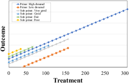
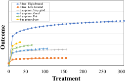
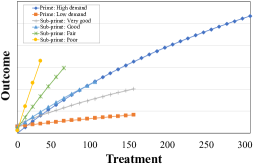
5.3.1 Visualization of ablation.
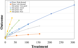
Now we visualize the prediction on six subgroups presented in Section 3 to intuitively illustrate the motivations of outcome regression and log transformation. More specifically, for each customer in the test set, the outcomes are predicted by different methods under all treatments, ranging from 0 to the corresponding maximum value with a stride of 1000. After averaging the predicted results for each subgroup, the average response curves are shown in Figure 3. First of all, although GBDT is the most popular method in machine learning and its performance is outstanding in many tasks, it has nearly no ability of interpolation, and thus cannot generalize to counterfactual predictions. Different from the simple linear regression, the outcome regression allows customers with different features having different marginal effects. After introducing the log transformation to the treatment, the marginal effects are able to decrease along with the increase of treatments, and the intensity of diminishing marginal effect is controlled by the hyper-parameter .
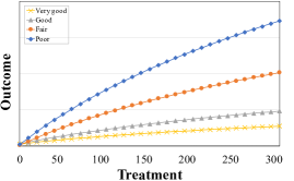
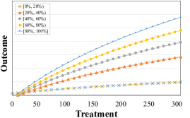
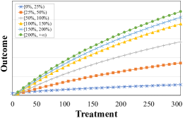
5.3.2 Partial dependence plots.
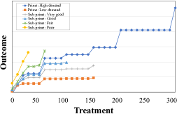
As we have the response model for each customer, the average response curve for any specific type of customers can be easily obtained by averaging their treatment effects. By inspecting the Partial Dependence Plots (PDP) for different types of customers, we could gain deeper insights into the industry trends. Therefore, the response models can not only help to determine the adjustment of credit limit for a particular customer, but also help to make better macro-decisions. In this subsection, we partition the customers into several groups according to three most important factors, and the PDPs for different types of customers are presented in Figure 4. As we can see, the marginal treatment effect is larger for customers with higher risk, probably because their current credit limits are quite low. For the customers with higher utilization or spends, it is likely that the current credit limits cannot cover their demands, and thus one unit increase of credit limit leads to higher growth of balance. All above observations are consistent with our expert experiences.
6 Conclusion
In this paper, we propose a data-driven approach based on causal inference to manage the credit limit in intelligent ways. Firstly, we design and conduct a conditional independence testing. Based on the acquired data from testing, a structural outcome regression model is built to measure the heterogeneous treatment effect of increasing credit limits. Through a carefully selected log transformation, the diminishing marginal effect has been incorporated. The capability of our model is further enhanced by applying GBDT encoding to features. Finally, we propose a proper evaluation metric to measure the performances of compared methods. The experimental results confirm the effectiveness of our approach and the analyses are inspiring.
For future works, there is a strong motivation to compare the performance between methods based on testing and methods based on observational study. If the difference is noteworthy, it is an interesting topic to investigate the possibility of reducing the gap.
References
- Addo et al. [2018] Peter Addo, Dominique Guegan, and Bertrand Hassani. Credit risk analysis using machine and deep learning models. Risks, 6(2):38, 2018.
- Athey and Imbens [2016] Susan Athey and Guido Imbens. Recursive partitioning for heterogeneous causal effects. Proceedings of the National Academy of Sciences, 113(27):7353–7360, 2016.
- Athey [2017] Susan Athey. Beyond prediction: Using big data for policy problems. Science, 355(6324):483–485, 2017.
- Dey [2010] Shubhamoy Dey. Credit limit management using action-effect models. In 2010 International Conference on Financial Theory and Engineering, pages 112–115. IEEE, 2010.
- Edin [2018] Moa Edin. Outcome regression methods in causal inference: The difference lasso and selection of effect modifiers, 2018.
- Gross et al. [2000] David B Gross, Nicholas Souleles, et al. Consumer response to changes in credit supply: Evidence from credit card data. Unpublished manuscript, University of Chicago and University of Pennsylvania, 2000.
- He et al. [2014] Xinran He, Junfeng Pan, Ou Jin, Tianbing Xu, Bo Liu, Tao Xu, Yanxin Shi, Antoine Atallah, Ralf Herbrich, Stuart Bowers, et al. Practical lessons from predicting clicks on ads at facebook. In Proceedings of the Eighth International Workshop on Data Mining for Online Advertising, pages 1–9. ACM, 2014.
- Hernan and Robins [2010] Miguel A Hernan and James M Robins. Causal inference, 2010.
- Hirano et al. [2003] Keisuke Hirano, Guido W Imbens, and Geert Ridder. Efficient estimation of average treatment effects using the estimated propensity score. Econometrica, 71(4):1161–1189, 2003.
- Hodson et al. [2014] Randy Hodson, Rachel E Dwyer, and Lisa A Neilson. Credit card blues: the middle class and the hidden costs of easy credit. The Sociological Quarterly, 55(2):315–340, 2014.
- Imbens and Rubin [2015] Guido W Imbens and Donald B Rubin. Causal inference in statistics, social, and biomedical sciences. Cambridge University Press, 2015.
- Jordà and Taylor [2016] Òscar Jordà and Alan M Taylor. The time for austerity: estimating the average treatment effect of fiscal policy. The Economic Journal, 126(590):219–255, 2016.
- Jordan and Mitchell [2015] Michael I Jordan and Tom M Mitchell. Machine learning: Trends, perspectives, and prospects. Science, 349(6245):255–260, 2015.
- Khandani et al. [2010] Amir E Khandani, Adlar J Kim, and Andrew W Lo. Consumer credit-risk models via machine-learning algorithms. Journal of Banking & Finance, 34(11):2767–2787, 2010.
- Machado et al. [2019] Cecilia Machado, Azeem M Shaikh, and Edward J Vytlacil. Instrumental variables and the sign of the average treatment effect. Journal of Econometrics, 2019.
- Morgan and Winship [2015] Stephen L Morgan and Christopher Winship. Counterfactuals and causal inference. Cambridge University Press, 2015.
- Paul and Biswas [2017] Uttiya Paul and Angshuman Biswas. Consumer credit limit assignment using bayesian decision theory and fuzzy logic–a practical approach. Journal of Management (JOM), 4(2), 2017.
- Pearl [2009] Judea Pearl. Causality. Cambridge university press, 2009.
- Peters et al. [2017] Jonas Peters, Dominik Janzing, and Bernhard Schölkopf. Elements of causal inference: foundations and learning algorithms. MIT press, 2017.
- Rona-Tas and Guseva [2018] Akos Rona-Tas and Alya Guseva. Consumer credit in comparative perspective. Annual Review of Sociology, 44:55–75, 2018.
- Rosenbaum and Rubin [1983] Paul R Rosenbaum and Donald B Rubin. The central role of the propensity score in observational studies for causal effects. Biometrika, 70(1):41–55, 1983.
- Rosenberg and Gleit [1994] Eric Rosenberg and Alan Gleit. Quantitative methods in credit management: a survey. Operations research, 42(4):589–613, 1994.
- Rubin [2005] Donald B Rubin. Causal inference using potential outcomes: Design, modeling, decisions. Journal of the American Statistical Association, 100(469):322–331, 2005.
- Sohn et al. [2014] So Young Sohn, Kyong Taek Lim, and Yonghan Ju. Optimization strategy of credit line management for credit card business. Computers & Operations Research, 48:81–88, 2014.
- Soman and Cheema [2002] Dilip Soman and Amar Cheema. The effect of credit on spending decisions: The role of the credit limit and credibility. Marketing Science, 21(1):32–53, 2002.
- Song [2011] Yonho Song. Study on the determination of the fair credit card limit. Proceedings of the Korea money and finance association conference, 2011.
- Thomas [2000] Lyn C Thomas. A survey of credit and behavioural scoring: forecasting financial risk of lending to consumers. International Journal of Forecasting, 2(16):149–172, 2000.
- Wager and Athey [2018] Stefan Wager and Susan Athey. Estimation and inference of heterogeneous treatment effects using random forests. Journal of the American Statistical Association, 113(523):1228–1242, 2018.