No Cosmic Rays from Curvature Oscillations during Structure Formation with $F(R)$-gravity

Abstract

The Starobinsky model of modified gravity suggested to explain dark energy may be also considered in the astrophysical context. Recently it has been pointed out that in contracting regions curvature oscillations around the GR value may lead to the production of high energy particles which contribute to the cosmic ray flux. We revisit these calculations in the Einstein frame and show that the continuous approximation for the matter density used in the original calculations is not valid. We show that this problem is generic in $F(R)$-gravity models introduced to describe the dark energy. We go beyond the approximation and find the rate of particle production to be negligible.

1 Introduction

Theories of modified gravity have been suggested as models capable of explaining the accelerated expansion of the present Universe. The model of $F(R)$-gravity proposed by Starobinsky [1] successfully describes an evolution of the late-time Universe imitating the cosmological constant. The corresponding action for gravity reads

$$S=-\frac{M_{\rm P}^{2}}{2}\int d^{4}x\sqrt{-g}\left(R+F(R)\right),$$ (1)

where the reduced Planck mass $M_{\rm P}$ is expressed via the Newtonian gravitational constant $G_{N}$ as follows $M_{\rm P}=\sqrt{8\,\pi/G_{N}}=2.4\times 10^{18}$ GeV, and

$$F(R)=\lambda R_{0}\left(\left(1+\frac{R^{2}}{R_{0}^{2}}\right)^{-n}-1\right)-\frac{R^{2}}{6\,m^{2}}\,.$$ (2)

Here $m$ is the maximal mass of additional scalar degree of freedom, scalaron, that appears in $F(R)$ gravity, and parameter $R_{0}$ fixes the scale of energy density associated with the cosmological constant $\rho_{\Lambda}$ at present, when the Hubble parameter equals $H_{0}=1.45\times 10^{-42}$ GeV,

$$R_{0}=-\frac{2}{\lambda}\frac{\rho_{\Lambda}}{M_{P}^{2}}\,=-\frac{6\,\Omega_{\Lambda}H_{0}^{2}}{\lambda}\;,$$ (3)

with $\Omega_{\Lambda}\equiv\rho_{\Lambda}/\rho_{c}$ and critical energy density $\rho_{c}$ determined by the Friedman equation,

$$3\,M_{\rm P}^{2}\,H_{0}^{2}=\rho_{c}\,.$$ (4)

The main question is how to distinguish $F(R)$-gravity from the cosmological constant and other Dark Energy models? One way is to probe the Dark Energy equation of state: $F(R)$-gravity may predict Dark Energy with time-dependent and even phantom pressure-to-density relation (see e.g. [2, 3, 4] for reviews). Another way is to look for possible observable effects in astrophysics.

$F(R)$-gravity is equivalent to the usual gravity and an additional scalar field with a non-trivial potential and coupling to matter fields. In papers [5, 6] it was pointed out that, in space regions with rising matter density, growing curvature oscillations decay into high energy particles, thus contributing to the Cosmic Ray spectrum. These oscillations are oscillations of classical scalaron field. In this paper we address a question: where do this scalaron oscillations come from? Usually, a scalar field oscillates around minimum if for some reason it is shifted or pushed from the vacuum. In papers [5, 6] the initial amplitude of the oscillations is arbitrary while actually there is no arbitrariness because the history of the expanding Universe exactly defines the initial conditions for the scalaron field. Namely, scalaron being massive in the early Universe, decays to the Standard model particles providing the absence of scalaron excitations at the present time. However, scalarons may be produced through the quantum processes [7]. We show below that numerical estimates in [5, 6], performed for the adopted there initial conditions, correspond to very unrealistic situation of huge number density (and noticeable energy density) of the present scalaron configuration.

Actually, as it was noticed in [5], the oscillations arise even if the field is adiabatically settled in the vacuum because the scalaron minimum itself moves with rising density. However, this oscillation source leads to parametrically smaller amplitudes than those considered in [5, 6] for relatively large densities. For matter densities close to the present dark energy (and for parameters in a particular region) the oscillations might contribute a noticeable amount to the energy density of Universe (this situation, if realistic, needs a special study). However, this energy density does not release as high energy particles. We revisit calculations of [5, 6] and obtain that the used approximation of homogeneous matter and scalaron field does not work in the region where significant particle production was predicted. We go beyond this approximations and estimate the realistic flux of produced cosmic rays to be negligible. Although we study only a particular model of $F(R)$ gravity the considered effects are expected to be generic for the $F(R)$ models aimed at describing the dark energy [3]. Such models provide the scalaron potential whose form depends on the background matter density. This leads to the scalaron oscillations entering to highly non-linear regime in which the homogeneous description can be invalid.

2 Scalaron density in contracting objects

Classical oscillations of scalaron field $\phi$ may be described in terms of scalaron condensate and the number density of scalarons $n_{\phi}$ is defined through the amplitude of oscillations as [8]

$$n_{\phi}=\omega\langle\phi^{2}\rangle\,.$$ (5)

Here $\phi$ is a canonically normalized scalaron field and $\omega$ is the energy of each particle in the condensate, i.e. the scalaron effective mass. It depends on the surrounding matter density $\rho_{m}$ as [7]

$$\omega=\frac{H_{0}}{\sqrt{2n\lambda(2n+1)}}\left(\frac{\rho_{m}}{\rho_{c}}\right)^{n+1}\left(\frac{\lambda}{2\Omega_{\Lambda}}\right)^{n+1/2}.$$ (6)

While an astrophysical object (i.e. halo) contracts, $\rho_{m}$ grows. In [5, 6] matter density $\rho_{m}$ changes linearly with time as $\rho_{m}=\rho_{m0}(1+t/t_{J})$ for $t<t_{J}$ with $t_{J}$ being the Jeans time of contraction.

The scalaron field is related to the scalar curvature and may be defined through the derivative $F^{\prime}(R)\equiv dF/dR$ as

$$\phi=\frac{\sqrt{6}}{2}M_{P}\log(1+F^{\prime}(R))\approx\frac{\sqrt{6}}{2}M_{P}F^{\prime}(R)\,.$$ (7)

The equations of motion for action (1) provide with the equation of motion for scalaron. It is convenient to write this equation in terms of dimensionless variables which first has been done in [9]. Later calculations in [5, 6] are performed in terms of variable $\xi$ connected with scalaron field $\phi$ as follows,

$$\xi=-\frac{1}{2\lambda n}\left(\frac{\rho_{m0}}{M_{P}^{2}R_{0}}\right)^{2n+1}\,F^{\prime}(R)=-\frac{1}{2\lambda n}\left(\frac{\lambda\rho_{m0}}{2\Omega_{\Lambda}\rho_{c}}\right)^{2n+1}\,F^{\prime}(R)\,.$$ (8)

The equation of motion for $\xi$, that defines the time dependence of scalaron field, reads [5]

$$\xi^{\prime\prime}+\frac{\rho_{m}}{\rho_{m0}}-y=0\,,$$ (9)

where $y=y(\xi)$ is obtained from the equation

$$\frac{1}{y^{2n+1}}-gy=\xi,~{}~{}g\equiv\frac{H_{0}^{2}}{2n\lambda m^{2}}\left(\frac{\rho_{m0}}{\rho_{c}}\right)^{2n+2}\left(\frac{\lambda}{2\Omega_{\Lambda}}\right)^{2n+1}\,.$$ (10)

Primes in (9) correspond to the derivatives with respect to dimensionless time $\tau\equiv m\sqrt{g}t$, and numerically $g\ll 1$.

The scalaron field $\phi$ may be expressed in terms of function $\xi$ by using (7) and (8)

$$\phi=\sqrt{6}\lambda nM_{P}\left(\frac{2\Omega_{\Lambda}\rho_{c}}{\lambda\rho_{m0}}\right)^{2n+1}\,\xi\,.$$ (11)

As it is shown in the paper [5] when initial conditions expected in General Relativity are imposed, $y=1$ (which implies for the scalaron to be in the minimum of the potential), the amplitude of $\xi$-oscillations becomes

$$\delta\xi=(\kappa-y_{0}^{\prime})(2n+1)^{3/2},~{}~{}\kappa=\sqrt{6\lambda n}\left(\frac{\rho_{m0}}{\rho_{c}}\right)^{-n-1/2}\left(\frac{\lambda}{2\Omega_{\Lambda}}\right)^{-n-1/2}.$$ (12)

Here (in the limit of small $g$) $y_{0}^{\prime}$ is proportional to the derivative of curvature $R$ and is considered as a free parameter in [5]. Since the case of $y_{0}^{\prime}=\kappa$ is recognized in [5] as fine tuning, the initial amplitude is found to be of order $\delta\xi=\kappa\,(2n+1)^{3/2}$. Putting all things together we obtain the initial energy density of the scalaron condensate:

$$\rho_{\phi}(t=0)=\langle\phi^{2}\rangle\,\omega^{2}(t=0)=9\lambda^{2}n^{2}(2n+1)^{2}\,M_{P}^{2}H_{0}^{2}\,\left(\frac{2\Omega_{\Lambda}}{\lambda}\right)^{4n+2}\left(\frac{\rho_{c}}{\rho_{m0}}\right)^{4n+1}.$$ (13)

Accounting for the Friedman equation (4) we estimate for the set of parameters considered in [5] ($n=2$, $\lambda=1$, $\kappa=0.04$) the initial scalaron energy density

$$\rho_{\phi}(t=0)=1.5\times 10^{-4}\,\rho_{c}\;,$$ (14)

that actually exceeds the radiation (CMB) energy density at present. However one cannot expect such a large contribution of scalarons because less than one particle inside the horizon may be created in the present (or recent) Universe, see [7]. Scalarons created in the very early Universe were very heavy (with mass $m$) and hence decayed to the SM particles. So the initial conditions in [5] seem to be irrelevant.

3 Relevant initial conditions for scalaron field

When density changes in a contracting object the form of scalaron potential changes: its minimum goes closer to $\phi=0$ and its mass rises. The initial condition $y_{0}^{\prime}=0$ in [6] implies that scalaron at $t=0$ is put into the moving minimum with zero ’velocity’. But actually we should expect that at $t<0$ (i.e. before the contraction starts) there were no excitations and scalaron was in the vacuum state. Also we should propose that in the real situation the contraction starts in a smooth way providing the adiabatic evolution near $t=0$ [7] and oscillations should be excited with the minimal possible amplitude. In what follows it is convenient to introduce dimensionless time $\tau=t/(\kappa t_{J})$, where $t_{J}$ is the Jeans time, and new variables

$$\bar{\xi}=\xi-\xi_{min}\,,$$ (15)

where

$$\xi_{min}=(1+\kappa\tau)^{-(2n+1)}\,.$$ (16)

So the adiabatic solution of the scalaron equation of motion derived in [5],

$$\bar{\xi}^{\prime\prime}+\Omega^{2}\bar{\xi}=-\xi_{min}^{\prime\prime}\,,$$ (17)

with such (zero) initial conditions that at $t=0$ one has $\bar{\xi}=0$, $\bar{\xi}^{\prime}=0$ looks to be the closest to the realistic physical situation. Here we use notations of paper [5],

$$\Omega\equiv\frac{(1+\kappa\tau)^{n+1}}{\sqrt{2n+1}},$$ (18)

and primes correspond to derivatives with respect to $\tau$.

Note that the source in the r.h.s. of (17) even with zero initial conditions leads to oscillations of $\bar{\xi}$. The adiabatic solution of (17) may be obtained by the standard technique in the form

$$\bar{\xi}=-\xi_{1}\,\int\xi_{2}\,\xi_{min}^{\prime\prime}\,d\tau+\xi_{2}\,\int\xi_{1}\,\xi_{min}^{\prime\prime}\,d\tau\,,$$ (19)

where

$$\xi_{1}=\frac{1}{\sqrt{\Omega}}\sin{\int\Omega d\tau}\,,~{}~{}\xi_{2}=\frac{1}{\sqrt{\Omega}}\cos{\int\Omega d\tau}\,.$$ (20)

The solution (19) may be rewritten in the form (s.f. eq. (12) of Ref. [5])

$$\bar{\xi}=\alpha(\tau)\sin{\left(\int\Omega d\tau+\delta(\tau)\right)}.$$ (21)

After some calculations one finds the amplitude $\alpha(\tau)$ of generated oscillations in the limit of small $\kappa\ll 1$,

$$\alpha(\tau)\simeq C_{n}\kappa^{2}(1+\kappa\tau)^{-\frac{n+1}{2}},~{}~{}C_{n}=2(n+1)\,(2n+1)^{2}\,.$$ (22)

This result corresponds to the initial amplitude of oscillations equal to $\alpha_{0}=C_{n}\kappa^{2}$, not of order $\kappa$ as it is proposed in [5]. We obtain parametrically smaller amplitude for matter densities much larger than the critical one $\rho_{m0}\gg\rho_{c}$ which are relevant for the astrophysical processes (star and galaxy formation). In Appendix we find the oscillations amplitude for more realistic Tolman model of spherical contraction in the expanding Universe. If the initial conditions are set in the early Universe, well before the moment when the contraction starts, one obtains much stronger (exponential) suppression of the scalaron oscillations for small enough $\kappa$. The evolution of the scalaron turns to be adiabatic in this limit.

However, for matter densities close to the critical one (cosmological processes), $\rho_{m0}\sim\rho_{c}$, the amplitude of oscillations may still be large, see eq. (11), providing a significant contribution to the energy density of the Universe (13) for some choice of parameters: e.g., $n=2$ and $\lambda\approx 1$. In this region of model parameter space the detailed analysis of theoretical consistency and phenomenological and cosmological viability of $F(R)$-model is needed.

As noted in [5, 6] scalaron oscillations may produce massless particles. But when $\xi>0$ (regular region, see eqs. (10), (9)) the process cannot be efficient because of very small effective scalaron mass. We show that using the approximation of decaying scalaron condensate which works perfectly well in the regular region. The scalaron density for the amplitude (22) is of order

$$\rho\sim M_{P}^{2}H_{0}^{2}\left(\frac{\rho_{m0}}{\rho_{c}}\right)^{-6n-2}.$$ (23)

We use the scalaron decay width to (massless) gauge bosons from [10], $\Gamma\sim\omega^{3}/M_{P}^{2}$, and estimate the energy density of particles created by scalaron oscillations during the Universe lifetime as

$$\rho_{p}\sim\frac{\rho\,\Gamma}{H_{0}}=H_{0}^{4}\,\left(\frac{\rho_{m0}}{\rho_{c}}\right)^{-3n+1},$$ (24)

which in any case means less than one particle in a horizon-size region. The reason here is clear, since $\omega\sim H_{0}$, the scalarons are stable at the cosmological time-scale, $\Gamma\sim H_{0}(H_{0}/M_{P})^{2}\ll H_{0}$. A similar result has been obtained in [6].

Only if $\xi$ becomes negative (in a spike region as it is called in [6]) its effective mass may increase because the scalaron potential at negative $\phi$ may be very steep. One observes from (12), (15), (16), (22), that the spike region can be reached on the Jeans time scale only for matter densities $\rho_{m}$ close to $\rho_{c}$, and hence is relevant only for the recent cosmic structure formation.

In the next Section 4 we estimate the flux of particles produced by scalaron oscillations in the spike region ($\xi<0$).

4 Particle production in the spike region

Hereafter we consider the case of matter densities $\rho_{m}$ close to $\rho_{c}$ which may help $\xi$ to reach negative values. In this region of parameters the time of contraction is very large, of order of the Universe age and the contraction has been started not long ago. So we are interested in the evolution only until $t_{J}$, and for that time one has $\Omega\kappa t\lesssim 1$, see Eq. (18), and $\xi$ reaches negative values only once or twice each time producing a spike in the solution for curvature [5, 6]. Below we estimate the particle production during one spike.

Homogeneous oscillations of classical scalaron field may produce non-conformal particles and production of scalars minimally coupled to gravity is the most efficient [11]. Scalaron is coupled to scalar field $h$ through the kinetic mixing in lagrangian [11]

$$L_{int}=\frac{h}{\sqrt{6}M_{P}}\partial_{\mu}\phi\,\partial^{\mu}h\,.$$ (25)

This coupling modifies the equation of motion for $h$:

$$\partial_{\mu}\partial^{\mu}h+\left(\frac{\ddot{\phi}}{\sqrt{6}M_{P}}+m_{h}^{2}\right)h=0\,,$$ (26)

where $m_{h}$ is the scalar mass. Scalaron field here plays a role of the external force producing particles $h$. The number of produced particles may be estimated by making use of the Bogoloubov transformations. From eq. (26) one obtains for the Fourier mode $h_{k}$ of 3-momentum $k$,

$$\ddot{h}_{k}+\left(k^{2}+m_{eff}^{2}(t)+m_{h}^{2}\right)h_{k}=0\,,$$ (27)

where $m_{eff}^{2}(t)=\ddot{\phi}/(\sqrt{6}M_{P})$.

Note that the spikes correspond to the negative values of $\phi$ and in that region the scalaron mass is maximal, so one has $\ddot{\phi}=-m^{2}\phi$ during the spike. The maximum value of $|\phi_{m}|$ may be extracted from the maximum $|\xi_{m}|$ estimated in [5]:

$$\frac{|\phi_{m}|}{\sqrt{6}M_{P}}=N\frac{H_{0}}{m}\left(\frac{\rho_{m0}}{\rho_{c}}\right)^{-n}z_{1}^{-n},~{}~{}N=\sqrt{\frac{\lambda}{2}}\left(\frac{2\Omega_{\Lambda}}{\lambda}\right)^{n+1/2}.$$ (28)

Here $z_{1}\equiv 1+t_{1}/t_{J}$ where $t_{1}$ corresponds to the moment when $\xi$ crosses zero for the first time: $\alpha(\tau_{1})=\xi_{min}(\tau_{1})$. Note that for the case we consider the variable $z$ is in the interval $1<z_{1}<2$, so we put it to be $z_{1}=1$ hereafter having in mind an upper bound. Then the maximum possible value of $m_{eff}^{2}(t)$ is

$$M^{2}=NmH_{0}\left(\frac{\rho_{m0}}{\rho_{c}}\right)^{-n}.$$ (29)

If we approximate the spike by the gaussian form with height of $M$ and width of $1/m$ we obtain formally that the spectrum has a cut off at high momenta of order $m$. The calculation shows that high energy particles with number density of order $n_{p}\sim M^{4}/m$ are produced by spike, in agreement with the statement of Ref. [5].

Since production of such energetic particles in a slow and smooth process of contraction looks very surprising from any point of view it is needed to check the validity of all approximations in use. The approximation that is certainly doubted is the homogeneous energy-momentum tensor for the background matter. If one considers a set of discrete particles instead of continuous medium one obtain that they produce the scalaron field like point sources. Every particle produces the field $\xi\propto e^{-\omega r}/r$ like the usual massive scalar with mass $\omega$. If the average distance $d$ between particles is large, $d\gg 1/\omega$, then the scalaron field is strongly inhomogeneous and approximation used for the energy-momentum tensor is not valid.

In this case we expect that the energetic particle production may still take place only in the small vicinities of the point sources, i.e. in very small spherical regions of radius $1/m$. Therefore, the total number of produced particles is suppressed by a very small number $n/m^{3}$ where $n$ is the matter number density. For the energy density we get the estimate

$$\rho\sim\frac{M^{4}\,n}{m^{3}}=N^{2}\rho_{m0}\,\frac{H_{0}^{2}}{m_{0}\,m}\left(\frac{\rho_{m0}}{\rho_{c}}\right)^{-2n},$$ (30)

where $m_{0}$ is the mass of particle populating the contracting object (region). For the interesting astrophysical objects and any regions dominated by baryons one puts $m_{0}\sim 1$ GeV. Then for the close to critical density and the scalaron mass $m\sim 10^{13}$ GeV we obtain $\rho\sim 10^{-92}~{}{\rm GeV/(cm^{2}\,s)}$ which is too small number to talk about.

Note in passing, though we discussed the particle production from one spike, the consideration of a sequence of several spikes does not significantly change the result. Another comment concerns the contraction of dark matter dominated region. To the case of particle-like dark matter (e.g. weakly interaction massive particles) the estimate (30) is applicable with $m_{0}$ referring to the dark matter particle mass. Say, for the galactic dark matter particle heavier than 1 eV the size of its wave packet (de Broglie wavelength corresponding to the average velocity $10^{-3}$) is smaller than the distance between particles, hence the homogeneous description fails. This problem is expected to be generic for $F(R)$ gravity models constructed to describe the dark energy. Typically, the effective scalaron mass can vary with the background matter density by many orders of magnitude. This happens because $F(R)$ functions contain two different mass scales: the present day Hubble parameter and the maximal scalaron mass which must be introduced to avoid singularities [12]. The latter is bounded from below as $m\gtrsim 10^{5}$ GeV [13]. Therefore, the scalaron degree of freedom can possess the similar dynamics including the non-linear oscillations (spike region). In this region the validity of the homogeneous description is questioned. Note that the same problem is also inherent in chameleon models [14, 15].

The case of homogeneous oscillating scalar field (e.g. axion-like) playing the role of the dark matter is actually inconsistent with the stability of the studied in [5, 6] $F(R)$-gravity (2). This model is known to be well defined only for $R\gtrsim R_{0}$ [12]. For lower values of $R$ the scalaron degree of freedom behaves as a tachyon. If the scalar field condensate dominates than the trace of the energy momentum tensor oscillates reaching negative values bringing the curvature to the region of instability. The same problem arising at the stage of inflaton oscillations was considered in detail in [12] (see Sec. 4.1 of that paper). This problem can be avoided with an appropriate choice of the function $F(R)$. However, we expect the scalaron dynamics to be strongly affected by the oscillating condensate. The corresponding effects need a special study which is beyond the scope of this paper. To conclude, the homogeneous approximation for the matter, as well as the results of [5, 6] for the efficient cosmic ray production in the spike region, are invalid for a generic dark matter model of this type.

To summarize, we have shown that contracting objects made of baryons or dark matter particles in $F(R)$-gravity do not contribute to the cosmic ray spectrum via the decay of the scalaron oscillations.

We thank E.Arbuzova, F.Bezrukov, A.Dolgov, D.Levkov, A.Panin, V.Rubakov and S.Sibiryakov for correspondence and discussions. The work has been supported by Russian Science Foundation grant 14-12-01430.

Appendix A The realistic model for the Jeans contraction during the structure formation

A structure formation process starts at the matter dominated stage. In the linear regime small perturbations grow as $\delta\rho/\rho\propto a\propto t^{2/3}$. When $\delta\rho/\rho$ reaches unity the non-linear contraction starts. For the spherically symmetric perturbations, the smooth transition between this two regimes may be approximately described by the Tolman solution [16]:

$$t=\sqrt{\frac{3}{8}}t_{J}(\zeta+\sin{\zeta}),~{}~{}\rho_{m}=\frac{8\rho_{m0}}{(1+\cos{\zeta})^{3}}~{}.$$ (31)

Here $t_{J}=1/\sqrt{4\pi G\rho_{m0}}$. The moment $t=0$ correspond to the time when the density starts to grow. This solution has two singularities: in the past and in the future. The singularity in the past corresponds to the Big Bang while the singularity in the future at $\zeta=\pi/2$ is never reached for real objects. Clearly, the solution is valid only for $t\lesssim t_{J}$.

The motivated initial conditions on the scalaron field must follow from the fact that all scalarons (if ever produced) had been decayed well before the matter dominated stage started. Therefore, the scalaron had been placed to the minimum and moved together with it adiabatically before the Jeans contraction started. Here we show that the resulting amplitude of scalaron oscillations is strongly suppressed compared to the case when the vacuum initial conditions are set at the moment when the contraction starts.

We numerically solve both equations (9) and (10) for the Tolman model of density evolution (31). As it is done in [5], we introduce the dimensionless parameter $\kappa=1/(m\sqrt{g}t_{J})$ and present plots for several choices of $\kappa$, see Fig. 1.

           

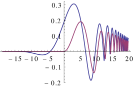
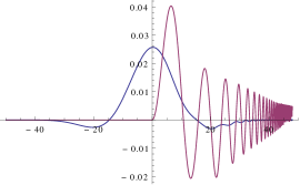
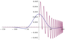
Figure 1: These plots show the evolution of $\xi-\xi_{min}$ for $\kappa=0.08$ (left), $\kappa=0.03$ (middle) and $\kappa=0.01$ (right). The blue line corresponds to initial conditions $\xi(\tau_{0})=\xi_{min}(\tau_{0})$, $\xi^{\prime}(\tau_{0})=\xi_{min}^{\prime}(\tau_{0})$ imposed at $\tau_{0}=-1.5/\kappa$, the violet line is for $\tau_{0}=0$. Taking the earlier initial time for the first choice of conditions provides with the same result.

The larger $\kappa$ correspond to the smaller minimal densities $\rho_{m0}$.

One observes in Fig. 1 that for relatively large realistic values of $\kappa$ we obtain larger amplitude of oscillations than for setting initial conditions at $\tau_{0}=0$. But for small $\kappa$ the late time oscillation amplitude becomes negligible compared to the case $\tau_{0}=0$. For the case $\tau_{0}=0$ we obtain that the final amplitude of induced oscillations behaves as $\kappa^{2}$ similarly to the results of the Sec. 3. From Fig. 1 (middle and right panels) it is seen that for more realistic choice of $\tau_{0}\sim-1/\kappa$ the amplitude drops with $\kappa$ much faster.

The exponential damping of the discussed effect for the small scale structures with densities much larger than the critical one can be understood analytically. The solution (19) of the linearised equation (17) can be rewritten in the form

$$\bar{\xi}=A(\tau)\sin{\left(\int\Omega d\tau+\delta(\tau)\right)},$$ (32)

where $\Omega$ is approximated as $\Omega=(1+\kappa^{2}\tau^{2}/6)^{n+1}/\sqrt{2n+1}$ for $\tau<1/\kappa$.

The amplitude $A(\tau)$ can be calculated as

$$A(\tau)=|\int^{\tau}_{-\infty}d\tau_{1}\,\xi_{min}^{\prime\prime}(\tau_{1})\frac{e^{i\int_{0}^{\tau_{1}}\Omega d\tau_{2}}}{\sqrt{\Omega}}|$$ (33)

The oscillations are generated near $\tau=0$. For $\tau>1/\kappa$ the impact of the source $\xi_{min}^{\prime\prime}$ becomes negligible so the amplitude is actually the same as in the formal limit $\tau\rightarrow\infty$. The latter is given by the integral

$$A=|\int^{\infty}_{-\infty}d\tau_{1}\,\xi_{min}^{\prime\prime}(\tau_{1})\frac{e^{i\int_{0}^{\tau_{1}}\Omega d\tau_{2}}}{\sqrt{\Omega}}|=|\int^{\infty}_{-\infty}d\tau_{1}\,\frac{e^{i\int_{0}^{\tau_{1}}\Omega d\tau_{2}}P(\kappa\tau)}{(1+\kappa^{2}\tau^{2}/6)^{\alpha}}|\,,$$ (34)

where $P(\kappa\tau)$ is some polynomial function, $\alpha=(5n+7)/2$. Calculating this integral with residues one finds the main exponential dependence:

$$A\propto e^{-\frac{\beta(n)}{\kappa}},\beta(n)=\frac{\sqrt{6\pi}\,\Gamma(n+2)}{2\sqrt{2n+1}\,\,\Gamma(n+5/2)}\,.$$ (35)

Thus, for small $\kappa$ oscillations are strongly suppressed, in agreement with the numerical calculations presented in Fig. 1.

References

- [1] A. A. Starobinsky, JETP Lett. 86, 157 (2007) [arXiv:0706.2041 [astro-ph]].
- [2] S. Nojiri and S. D. Odintsov, eConf C 0602061 (2006) 06 [Int. J. Geom. Meth. Mod. Phys. 4 (2007) 115] [hep-th/0601213].
- [3] T. P. Sotiriou and V. Faraoni, Rev. Mod. Phys. 82, 451 (2010) [arXiv:0805.1726 [gr-qc]].
- [4] S. Nojiri and S. D. Odintsov, Phys. Rept. 505 (2011) 59 [arXiv:1011.0544 [gr-qc]].
- [5] E. V. Arbuzova, A. D. Dolgov and L. Reverberi, Eur. Phys. J. C 72, 2247 (2012) [arXiv:1211.5011 [gr-qc]].
- [6] E. V. Arbuzova, A. D. Dolgov and L. Reverberi, Phys. Rev. D 88, no. 2, 024035 (2013) [arXiv:1305.5668 [gr-qc]].
- [7] D. Gorbunov and A. Tokareva, J. Exp. Theor. Phys. 120, no. 3, 528 (2015) doi:10.1134/S1063776115030085 [arXiv:1412.3413 [astro-ph.CO]].
- [8] D. S. Gorbunov and V. A. Rubakov, Hackensack, USA: World Scientific (2011) 489 p
- [9] E. V. Arbuzova and A. D. Dolgov, Phys. Lett. B 700, 289 (2011) [arXiv:1012.1963 [astro-ph.CO]].
- [10] D. Gorbunov and A. Tokareva, JCAP 1312, 021 (2013) [arXiv:1212.4466 [astro-ph.CO]].
- [11] D. S. Gorbunov and A. G. Panin, Phys. Lett. B 700, 157 (2011) [arXiv:1009.2448 [hep-ph]].
- [12] S. A. Appleby, R. A. Battye and A. A. Starobinsky, JCAP 1006, 005 (2010) [arXiv:0909.1737 [astro-ph.CO]].
- [13] E. V. Arbuzova, A. D. Dolgov and L. Reverberi, JCAP 1202, 049 (2012) [arXiv:1112.4995 [gr-qc]].
- [14] J. Khoury, Class. Quant. Grav. 30, 214004 (2013) [arXiv:1306.4326 [astro-ph.CO]].
- [15] C. Burrage and J. Sakstein, arXiv:1709.09071 [astro-ph.CO].
- [16] V. Mukhanov, “Physical Foundations of Cosmology”, Cambridge University Press (2005)