Superfluid Mutual-friction Coefficients from Vortex Dynamics in the Two-dimensional Galerkin-truncated Gross-Pitaevskii Equation

Abstract

We present algorithms for the ab-initio determination of the temperature ($T$) dependence of the mutual-friction coefficients $\alpha$ and $\alpha^{\prime}$ and the normal-fluid density $\rho_{\rm n}$ in the two-dimensional (2D) Galerkin-truncated Gross-Pitaevskii system. Our algorithms enable us to determine $\alpha(T)$, even though fluctuations in 2D are considerably larger than they are in 3D. We also examine the implications of our measurements of $\alpha^{\prime}(T)$ for the Iordanskii force, whose existence is often questioned.

The elucidation of the statistical properties of superfluid turbulence and the comparison of these with their fluid-turbulence analogs is a problem of central importance that lies at the interface between fluid dynamics and statistical mechanics Vinen (2000); Skrbek and Sreenivasan (2012). Theoretical treatments of superfluid turbulence use a variety of models Berloff et al. (2014); Barenghi et al. (2014); Proukakis and Jackson (2008), which are applicable at different length scales and for different interaction strengths. At low temperatures $T$ and for weakly interacting bosons, the Gross-Pitaevskii (GP) equation provides a good hydrodynamical description of a superfluid with quantum vortices. If we consider length scales that are larger than the mean separation between quantum vortices, and if we concentrate on low-Mach-number flows, then the two-fluid model Donnelly (1991); Khalatnikov (1965) of Hall, Vinen, Bekharevich, and Khalatnikov (HVBK) provides a good description of superfluid turbulence. In the HVBK equations, the normal and superfluid velocities are coupled by two mutual-friction coefficients, $\alpha$ and $\alpha^{\prime}$. The determination of $\alpha$ and $\alpha^{\prime}$, along with the normal-fluid density $\rho_{\rm n}$, as functions of $T$, from (a) experiments Donnelly (1991); Barenghi et al. (1983); Donnelly and Barenghi (1998), (b) kinetic models Griffin et al. (2009); Proukakis and Jackson (2008); Berloff et al. (2014), or (c) the Galerkin-truncated GP equation Krstulovic and Brachet (2011a); Shukla et al. (2013) is a challenging problem. Such studies have been carried out only in three dimensions (3D). Given that (a) two-dimensional (2D) and 3D fluid turbulence are qualitatively different Boffetta and Ecke (2012); Pandit et al. (2009) and (b) 2D and 3D superfluids are also qualitatively different Kogut (1979); Minnhagen (1987), it behooves us to carry out GP-based investigations of $\alpha$ and $\alpha^{\prime}$ for a 2D superfluid.

We present the first calculation of $\alpha(T),\alpha^{\prime}(T)$, and $\rho_{\rm n}(T)$ in the 2D Galerkin-truncated GP system. The determination of $\alpha(T),\alpha^{\prime}(T)$, and $\rho_{\rm n}(T)$ turns out to be considerably more challenging in 2D than in 3D Krstulovic and Brachet (2011a) because of large fluctuations. We obtain the dependence of $\alpha(T),\alpha^{\prime}(T)$, and $\rho_{\rm n}(T)$ on $T$ by using an algorithm, which allows us to examine the evolution of vortical configurations, such as, a pair of vortices and a quadruplet of vortices, placed initially at the corners of a square. We find that $\alpha^{\prime}(T)$ is smaller than $\alpha(T)$ in magnitude, but nonzero; this suggests that the Iordanskii force Thouless et al. (1996); Volovik (1996); Wexler (1997); Hall and Hook (1998); Sonin (1998); Wexler et al. (1998); Fuchs et al. (1998), whose existence has often been questioned, does not vanish.

The Galerkin-truncated GP equation for the complex, classical field $\psi(\mathbf{x},t)$ of a weakly interacting 2D Bose gas is

$$i\frac{\partial\psi(\mathbf{x},t)}{\partial t}=\mathcal{P}_{G}\Bigl{[}-\alpha_{0}\nabla^{2}\psi(\mathbf{x},t)+g\mathcal{P}_{G}[|\psi|^{2}]\psi(\mathbf{x},t)\Bigr{]},$$ (1)

where $g$ is the effective interaction strength, the Galerkin projector $\mathcal{P}_{G}[\hat{\psi}(k)]=\theta(k_{\rm max}-k)\hat{\psi}(k)$, with $\hat{\psi}$ the Fourier transform of $\psi$ and $\theta(\cdot)$ the Heaviside function. This truncated GP equation (TGPE) conserves the total energy $H=2\alpha_{0}\int_{\mathcal{A}}d^{2}x(\alpha_{0}|\nabla\psi|^{2}+\frac{g}{2}[\mathcal{P}_{G}|\psi|^{2}]^{2})$, the total number of particles $N=\int_{\mathcal{A}}d^{2}x|\psi|^{2}$, and the momentum $\mathbf{P}=\alpha_{0}\int_{\mathcal{A}}d^{2}x(\psi\nabla\psi^{*}-\psi^{*}\nabla\psi)$. The Madelung transformation $\psi=\sqrt{\rho(\mathbf{x},t)}\exp(i\phi)$, where $\rho$ and $\phi$ are the density and phase field, respectively, yields the velocity $\mathbf{v}=2\alpha_{0}\nabla\phi$, with the quantum of circulation $4\pi\alpha_{0}$, the sound velocity $c=\sqrt{g\rho^{*}}$, the healing length $\xi=\sqrt{2\alpha_{0}^{2}/(g\rho^{*})}$, the total density $\rho^{*}=N/\mathcal{A}$, and $\mathcal{A}=L^{2}$ is the area of our 2D, periodic, computational domain of side $L=2\pi$ (see the Supplemental Material sup for units). We use the $2/3$ dealiasing rule in our pseudospectral direct numerical simulation (DNS) of the TGPE, with the maximum wave number $k_{max}=2/3\times N_{c}/2$, where $N_{c}^{2}$ is the number of collocation points Krstulovic and Brachet (2011a). This scheme ensures global-momentum conservation in our DNSs and it is essential for capturing accurately the interactions of the normal fluid with the superfluid vortices Krstulovic and Brachet (2011a). We use a fourth-order, Runge-Kutta scheme, with time step $\Delta t$, for time marching.

Generic initial conditions evolve slowly, under the 2D TGPE dynamics, towards equilibrium in the microcanonical ensemble Shukla et al. (2013): the system goes through initial transients, then displays the onset of thermalization, which is followed by a regime of partial thermalization, and then complete thermalization, with a low-$T$ Berezinskii-Kosterlitz-Thouless (BKT) phase, a high-$T$ phase with unbound vortices, and a transition between these phases at $T_{\rm BKT}$. To accelerate equilibration and to have direct control over (a) $T$, for the desired equilibrium state, and (b) states with counterflows, we use the generalized grand canonical ensemble with the equilibrium probability distribution $\mathbb{P}[\psi]=\Xi^{-1}\exp[-\beta(H-\mu N-\mathbf{w}\cdot\mathbf{P})]$, where $\Xi$ is the grand partition function, $\beta=T^{-1}$ (we set the Boltzmann constant $k_{B}=1$), $\mu$ the chemical potential, $\mathbf{w}=\mathbf{v}_{n}-\mathbf{v}_{s}$ the counterflow velocity, and $\mathbf{v}_{n}$ and $\mathbf{v}_{s}$ the normal and superfluid velocities, respectively. We construct a stochastic process, which leads to this $\mathbb{P}[\psi]$, via the 2D stochastic Ginzburg-Landau equation (SGLE)

$$\frac{\partial\psi}{\partial t}=\mathcal{P}_{G}\Bigl{[}\alpha_{0}\nabla^{2}\psi-g\mathcal{P}_{G}[|\psi|^{2}]\psi+\mu\psi-i\mathbf{w}\cdot\nabla\psi+\zeta(\mathbf{x},t)\Bigr{]},$$ (2)

where $\zeta$ is a zero-mean, Gaussian white noise with $\langle\zeta(\mathbf{x},t)\zeta^{*}(\mathbf{x}^{\prime},t^{\prime})\rangle=D\delta(\mathbf{x}-\mathbf{x}^{\prime})\delta(t-t^{\prime})$, $\delta$ the Dirac delta function, and $D=1/(2\alpha\beta)$, in accordance with the fluctuation-dissipation theorem. We solve this SGLE along with

$$\frac{d\mu}{dt}=-\frac{\nu_{N}}{\mathcal{A}}(N-N_{av}),$$ (3)

so that $N_{av}$ controls the mean value of $N$ and $\nu_{N}$ governs the rate at which the SGLE equilibrates. The counterflow term $i\mathbf{w}\cdot\nabla\psi$ yields states with a non-vanishing $\mathbf{w}$.

In the HVBK model Donnelly (1991); Barenghi et al. (1983); Shukla et al. , a superfluid vortex does not move with the superfluid velocity $\mathbf{v}_{\rm s}$ but with velocity

$$\mathbf{v}=\mathbf{v}_{\rm sl}+\alpha\mathbf{s}^{\prime}\times(\mathbf{v}_{\rm n}-\mathbf{v}_{\rm sl})-\alpha^{\prime}\mathbf{s}^{\prime}\times[\mathbf{s}^{\prime}\times(\mathbf{v}_{\rm n}-\mathbf{v}_{\rm sl})],$$ (4)

where $\mathbf{v}_{\rm sl}=\mathbf{v}_{\rm s}+\mathbf{v}_{\rm si}$ is the local superfluid velocity, with $\mathbf{v}_{\rm s}$ and $\mathbf{v}_{\rm si}$ the imposed superfluid velocity and the self-induced velocity because of the vortices, respectively, and $\mathbf{s}^{\prime}$ the unit tangent at a point on the vortex, with position vector $\mathbf{s}$ . We use the following two initial configurations in the 2D TGPE: (1) $\psi_{\tt IC1}=\psi_{\rm pair}\psi_{\rm eq}$; and (2) $\psi_{\tt IC2}=\psi_{\rm lattice}\psi^{\rm cf}_{\rm eq}$. We obtain $\psi_{\tt IC1}$ by (a) first preparing a state $\psi_{\rm pair}$, which corresponds to a small, vortex-antivortex pair translating with a constant velocity along the $x$ direction (Supplemental Material sup ) and (b) then combining it with an equilibrium state $\psi_{\rm eq}$ to include finite-temperature effects (Supplemental Material sup ). To obtain $\psi_{\tt IC2}$, we first prepare $\psi_{\rm lattice}$, in which we place vortices of alternating signs on the corners of a square (a vortex lattice by virtue of the periodic boundary conditions) (Supplemental Material sup ); and then we include finite-temperature and counterflow effects by multiplying $\psi_{\rm lattice}$ with the state $\psi^{\rm cf}_{\rm eq}$ (Supplemental Material sup ). We obtain $\psi_{\rm eq}$ and $\psi^{\rm cf}_{\rm eq}$ by solving the SGLE (2); and then we use $\psi_{\tt IC1}$ to determine $\alpha(T)$ and $\psi_{\tt IC2}$ to calculate both $\alpha(T)$ and $\alpha^{\prime}(T)$.

Our DNS of the TGPE Eq. (1) yields the spatiotemporal evolutions of $\psi_{\tt IC1}$ and $\psi_{\tt IC2}$. We take $\mathbf{w}=v_{n}\hat{x}$ for all our SGLE DNSs with counterflows. Parameters for our DNSs are summarized in Table 1. We first plot the $x$ component of the momentum $P_{x}$ versus $v_{n}$, for five representative values of $T/\tilde{T}_{\rm BKT}$ (Fig. 1(a)), whence we obtain

$$\rho_{\rm n}(T)=\frac{1}{\mathcal{A}}\frac{\partial P_{\rm x}}{\partial v_{\rm n}}|_{v_{\rm n}=0},$$ (5)

whose values we list in column $3$ of Table 1. In Fig. 1(b), we plot, versus the scaled temperature $T/\tilde{T}_{\rm BKT}$, where $\tilde{T}_{\rm BKT}$ is a rough, energy-entropy-argument estimate of the BKT transition temperature Kogut (1979); Minnhagen (1987), $\rho_{\rm n}$ (green curve), $(1-\rho_{\rm n})$ (sky-blue curve), and the condensate fraction $N_{0}/N$ (purple line), where $N_{0}$ is the population of the zero-wave-number mode.

	$T/\tilde{T}_{\rm BKT}$	$\rho_{\rm n}$	$\alpha_{\tt IC1}$	$w$	$\alpha_{\tt IC2}$	$\alpha^{\prime}_{\tt IC2}$
R1	$6.37\times 10^{-4}$	$2.7\times 10^{-4}$	$(2\pm 1)\times 10^{-6}$	$0.8$	$2.5\times 10^{-5}$	$-2.2\times 10^{-5}$
R2	$3.19\times 10^{-3}$	$1.37\times 10^{-3}$	$(1.0\pm.3)\times 10^{-4}$	$0.8$	$1.8\times 10^{-4}$	$-1.5\times 10^{-4}$
R3	$6.37\times 10^{-3}$	$2.7\times 10^{-3}$	$(2.2\pm.6)\times 10^{-4}$	$0.6$	$3.6\times 10^{-4}$	$-1.8\times 10^{-4}$
R4	$3.19\times 10^{-2}$	$1.39\times 10^{-2}$	$(1.6\pm.5)\times 10^{-3}$	$0.4$	$2.3\times 10^{-3}$	$-4.5\times 10^{-4}$
R5	$6.37\times 10^{-2}$	$2.85\times 10^{-2}$	$(4\pm 1)\times 10^{-3}$	$0.2$	$6.9\times 10^{-3}$	$4.0\times 10^{-4}$
R6	$9.56\times 10^{-2}$	$4.37\times 10^{-2}$	$-$	$0.1$	$1.2\times 10^{-2}$	$-1.2\times 10^{-3}$
R7	$1.20\times 10^{-1}$	$5.97\times 10^{-2}$	$(1.2\pm.6)\times 10^{-2}$	$0.1$	$1.6\times 10^{-2}$	$2.9\times 10^{-3}$
R8	$1.59\times 10^{-1}$	$7.66\times 10^{-2}$	$-$	$0.1$	$1.4\times 10^{-2}$	$4.2\times 10^{-3}$
R9	$1.78\times 10^{-1}$	$8.71\times 10^{-2}$	$-$	$0.1$	$2.2\times 10^{-2}$	$-3.5\times 10^{-3}$

Table 1: Mutual-friction results from our DNS runs $\tt R1$-$\tt R9$: $T/\tilde{T}_{\rm BKT}$ is the scaled temperature; $\tilde{T}_{\rm BKT}=1.57\times 10^{-2}$ is the energy-entropy-argument based estimate of the BKT transition temperature; $\rho_{\rm n}$ is the normal-fluid density; $\mathbf{w}=v_{n}\hat{x}$ is the counterflow velocity; $\alpha$ and $\alpha^{\prime}$ are the mutual friction coefficients, where the subscripts $\tt IC1$ and $\tt IC2$ denote the initial configurations. In all our DNS runs, the total average density $\rho^{*}=N/\mathcal{A}=1$, the total number of collocation points $N_{c}^{2}=128^{2}$, the healing length $\xi=1.44\Delta x$, $\Delta x=2\pi/N_{c}$, the speed of sound $c=1$, and the quantum of circulation $\alpha_{0}\simeq 0.05$ are kept fixed.

We begin with our results for the spatiotemporal evolution of $\psi_{\tt IC1}=\psi_{\rm pair}\psi_{\rm eq}$. The vortex-antivortex pair in $\psi_{\rm pair}$, have centers that are separated, initially, by the small distance $d(t=0)\simeq 5.4\xi$ in the $y$ direction; the pair moves at a constant velocity $v_{\rm pair}=0.2775\hat{x}$. The state $\psi_{\rm eq}$, which is an absolute-equilibrium state at a temperature $T<T_{\rm BKT}$, provides the normal fluid that interacts with this vortex-antivortex pair and leads to a decrease in $d$ as time increases. In the Supplemental Material sup we show that

$$\mathrm{d}d^{2}/\mathrm{d}t=-8\alpha_{0}(1-\alpha^{\prime})\alpha;$$ (6)

we can neglect $\alpha^{\prime}$ here (as we show below, $\alpha^{\prime}\ll 1$). Thus, we can obtain $\alpha(T)$ from the slope of a straight-line fit to a plot of $d^{2}$ versus $t$. We determine $d^{2}(t)$ by tracking the positions of the vortices and thus obtain plots such as those shown in Fig. 2 for two representative values of $T/\tilde{T}_{\rm BKT}$ (DNS runs $\tt R2$ and $\tt R4$ in Table 1). The Video $\tt M1$, for the DNS run $\tt R2$, shows, via pseudocolor plots, the spatiotemporal evolution of the field $|\psi(\mathbf{x},t)|^{2}$: the vortex-antivortex pair moves under the combined influence of its initial momentum and the finite-temperature fluctuations, the average value of $d$ decreases with time and, finally, this pair disappears from the system (on time scales that are much longer than those shown in this video). From the plots in Fig. 2 we see that (a) $d^{2}$ fluctuates significantly in time and (b) these fluctuations increase with $T/\tilde{T}_{\rm BKT}$ (compare Figs. 2(a) and (b)). Thus, the higher the temperature, the more these fluctuations limit our ability to determine $d^{2}$ reliably, with averages over a fixed number of realizations of $\psi_{\rm eq}$, which we must limit, perforce, because of the computational cost of these calculations. We obtain $10$ values of $\alpha(T)$, because we use $10$ realizations of $\psi_{\rm eq}$. The mean of these values yield the value of $\alpha(T)$ that we have listed in column $4$ of Table 1; the standard deviations yield the error bars; $\alpha$ increases with $T$ (over the range we consider).

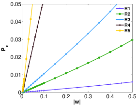
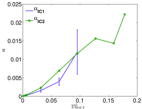
Figure 1: (Color online) Plots of (a) the momentum $P_{\rm x}$ versus the applied counterflow velocity $w$ for the DNS runs $\tt R1$-$\tt R5$; (b) the condensate fraction $N_{0}/N$ (purple line), the normal fluid density $\rho_{\rm n}$ (green line), and $1-\rho_{\rm n}$ (sky-blue line) versus $T/\tilde{T}_{BKT}$; (c) the mutual friction coefficients $\alpha_{\tt IC1}$ (purple line) and $\alpha_{\tt IC2}$ (green line) versus $T/\tilde{T}_{BKT}$; (d) $B=2\alpha/\frac{\rho_{n}}{\rho}$ versus $T/\tilde{T}_{BKT}$. Here the subscripts on $\alpha$ refer to the initial conditions $\tt IC1$ and $\tt IC2$.

\begin{overpic}[height=113.81102pt,unit=1mm]{figure2a.eps} \put(10.0,10.0){\large{\bf(a)}} \put(42.0,35.0){\large{\tt R2}} \end{overpic}\begin{overpic}[height=113.81102pt,unit=1mm]{figure2b.eps} \put(10.0,10.0){\large{\bf(b)}} \put(42.0,35.0){\large{\tt R4}} \end{overpic}

Figure 2: (Color online) Plots of the square of the vortex-pair length $d^{2}/\xi^{2}$ versus time $ct/\xi$ from our DNS runs: (a) $\tt R2$ at $T/\tilde{T}_{\rm BKT}=3.19\times 10^{-3}$; (b) $\tt R4$ at $T/\tilde{T}_{\rm BKT}=3.19\times 10^{-2}$. For each plot, the different solid lines indicate the time evolution of $d^{2}/\xi^{2}$ for the different realizations of $\psi_{\rm eq}$, which we obtain from the steady state of the SGLE. To reduce the noise in the plots of $d^{2}$, for these different realizations we have used a moving-average-based smoothening procedure (the function smooth in Matlab^®); this procedure introduces slight artifacts (high or low values of $d^{2}$) near the lowest and highest values of $t$ in these plots. To obtain $\alpha(T)$, we use the average of all the plots of $d^{2}$ versus $t$ (dashed black curve), at given value of $T$. The orange dashed line, a linear fit to this curve, is shown to guide the eye.

The state $\psi_{\rm lattice}$ consists of a quadruplet of alternating vortices and antivortices on the vertices of a square with sides of length $\pi$; for this state, the self-induced velocity $\mathbf{v}_{\rm si}$, because of these vortices and antivortices, is zero at $T=0$. In $\psi_{\tt IC2}$ we combine $\psi_{\rm lattice}$ with the thermalized state $\psi^{\rm cf}_{\rm eq}$, at different values of $T/\tilde{T}_{BKT}$ and counterflow velocity $\mathbf{w}=v_{n}\hat{x}$. Figures 3(a) and (b) show pseudocolor plots of the density field, for our DNS run $\tt R2$ at $T/\tilde{T}_{\rm BKT}=3.19\times 10^{-3}$ and $v_{n}=0.8$, at two different times $t=0$ and $t=1000$. Figures 3(a) and (b) and the corresponding Video $\tt M2$ show that the vortex lattice drifts under the influence of the imposed counterflow. Initially the vortex-lattice has an adaptation time period, during which a perpendicular motion, with a negligibly small velocity, and a drift, parallel to the applied counterflow, yield a vortex lattice imperfection, which we quantify by $\delta=\frac{1}{4}[(\delta y_{2}+\delta y_{4})-(\delta y_{1}+\delta y_{3})]$, where $\delta y_{i}$ is the $y$-displacement of the vortex $i$ (see Fig. 4(a) inset); the drift parallel to the applied counterflow is given by $\delta x=\frac{1}{4}(\delta x_{1}+\delta x_{2}+\delta x_{3}+\delta x_{4})$, with $\delta x_{i}$ the $x$-displacement of the vortex $i$. The imperfection $\delta(t)$ increases with $t$ and results in a self-induced velocity $\mathbf{v}_{\rm si}$, which leads to a decrease in the effective counterflow $w(t)$ because of the conservation of the total momentum. We develop a phenomenological model, which accounts for this effect (Supplemental Material sup ) and yields

$$\delta(t)=\frac{\rho_{n}w_{0}}{\alpha_{0}(\chi_{v}\rho_{n}+\chi_{p}\rho)}\biggl{(}1-\exp\bigl{[}-\frac{\alpha\alpha_{0}(\chi_{v}\rho_{n}+\chi_{p}\rho)}{\rho_{n}}t\bigr{]}\biggr{)}$$ (7)

and

$$\begin{split}\delta x(t)&=\biggl{(}\bigl{[}\chi_{v}\rho_{n}-\alpha^{\prime}(\chi_{v}\rho_{n}+\chi_{p}\rho)\bigr{]}\times\\ &\exp\bigl{[}-\frac{\alpha\alpha_{0}(\chi_{v}\rho_{n}+\chi_{p}\rho)}{\rho_{n}}t\bigr{]}-\chi_{v}\rho_{n}\\ &+(\chi_{v}\rho_{n}+\chi_{p}\rho)(\alpha^{\prime}+\alpha\alpha_{0}t)\biggr{)}\frac{\rho_{n}w_{0}}{\alpha\alpha_{0}(\chi_{v}\rho_{n}+\chi_{p}\rho)^{2}},\end{split}$$ (8)

where $w_{0}$ is the counterflow velocity at $t=0$; $\chi_{v}$ and $\chi_{p}$ are the proportionality constants given by $v_{\rm si}(\delta)=\chi_{v}\alpha_{0}\delta$ and $P_{\rm si}(\delta)=4\pi^{2}\chi_{P}\alpha_{0}\rho\delta$, where $P_{\rm si}$ is the self-induced momentum from the vortex-lattice imperfection. We determine $\alpha(T)$ and $\alpha^{\prime}(T)$ from the fits, suggested by the forms in Eqs. (7) and (8), to the plots of $\delta$ and $\delta x$, which we obtain from our DNS runs $\tt R1$-$\tt R9$ at different temperatures [details in the Supplemental Material sup ]. Figures 4(a) and (b) contain plots versus $t$ of $\delta(t)$ and $\delta x(t)$, respectively; Fig. 4(a) shows the saturation, at large $t$, of the vortex-lattice imperfection. The values of $\alpha(T)$ and $\alpha^{\prime}(T)$ that we obtain are listed in columns $6$ and $7$ of Table 1 for different values of $T/\tilde{T}_{BKT}$. It is reassuring to note that the values we obtain for $\alpha(T)$ from configurations $\tt IC1$ and $\tt IC2$ (columns $4$ and $6$) agree with each other.

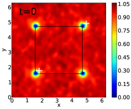
Figure 3: (Color online) Pseudocolor plots of the density field $|\psi(\mathbf{x},t)|^{2}$ from our DNS run $\tt R2$ at two different instants of time: (a) $t=0$ and (b) $t=1000$; these show the drift of the vortex crystal under the imposed counterflow $v_{n}=0.8\hat{x}$ at $T/\tilde{T}_{\rm BKT}=3.19\times 10^{-3}$. The $+$ and $-$ symbols (in white) show the signs of the vortices; and the black frame indicates the square at whose corners we place $\pm$ vortices at $t=0$. The Video $\tt M2$ shows, via pseudocolor plots, the spatiotemporal evolution of $|\psi(\mathbf{x},t)|^{2}$.

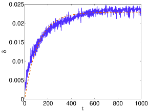
Figure 4: (Color online) Plots versus time $t$ of (a) the imperfection $\delta=\frac{1}{4}[(\delta y_{2}+\delta y_{4})-(\delta y_{1}+\delta y_{3})]$ and (b) the drift $\delta x=\frac{1}{4}(\delta x_{1}+\delta x_{2}+\delta x_{3}+\delta x_{4})$, from our DNS run $\tt R2$. The orange-dashed lines indicate the fits obtained by the use of Eqs. (7) and (8) (see text). Inset: a schematic diagram of the vortex-lattice imperfection; the square shows the shape of the vortex lattice at $t=0$.

The measurement of $\alpha^{\prime}(T)$ in 2D is difficult because of the following reasons: (1) at low temperatures its magnitude is small; (2) at high temperatures there are large thermal fluctuations that lead to large and noisy oscillations of the vortex lattice. Even though an accurate determination of $\alpha^{\prime}(T)$ is difficult, we find that $\alpha^{\prime}(T)$ is always nonzero and smaller in magnitude than $\alpha(T)$. For similar studies in the 3D GPE we refer readers to Refs. Berloff and Youd (2007); Krstulovic and Brachet (2011a, b). In particular, Ref. Jackson et al. (2009) has studied $\alpha(T)$ and $\alpha^{\prime}(T)$ in a pancake-type condensate.

We have shown how to obtain $\alpha(T),\alpha^{\prime}(T)$, and $\rho_{\rm n}(T)$, for 2D superfluids, by using the 2D Galerkin-truncated GP system. Even though the determination of $\alpha(T),\alpha^{\prime}(T)$, and $\rho_{\rm n}(T)$ is difficult, we succeed in calculating them for $T/\tilde{T}_{\rm BKT}\lesssim 10^{-1}$. At such low temperatures, the difference between the superfluid density $\rho_{s}$, which should be obtained strictly by using a helicity modulus Fisher et al. (1973); Kogut (1979); Minnhagen (1987), and $(1-\rho_{n})$ should not be significant in typical, laboratory-scale systems; and the HVBK model, with the values of $\alpha(T),\alpha^{\prime}(T)$, and $\rho_{\rm n}(T)$ that we have listed in Table 1, should provide a good description of the dynamics of 2D superfluids so long as we probe scales that are larger than the mean separation between quantum vortices. The existence of the Iordanskii force, which is related to the third term on the right-hand side of Eq.(4), has been the subject of a debate in the latter half of the 1990s Thouless et al. (1996); Volovik (1996); Wexler (1997); Hall and Hook (1998); Sonin (1998); Wexler et al. (1998); Fuchs et al. (1998). This force is linked to the asymmetry of the scattering of quasiparticles by a vortex Iordanskii (1966, 1965); and, if it is present, it implies that $\alpha^{\prime}$ is nonzero. Thus, given that we find $\alpha^{\prime}\neq 0$, our calculations imply that there is a nonvanishing Iordanskii force. To settle conclusively the issue of the existence of the Iordanskii force, we must obtain error bars on $\alpha^{\prime}(T)$; given the large fluctuations we have mentioned, the computational cost of obtaining such error bars is prohibitively large. We hope our study will lead to experimental measurements of $\alpha(T),\alpha^{\prime}(T)$, and $\rho_{\rm n}(T)$ in 2D superfluids, whose analogs for 3D superfluids Barenghi et al. (1983) have been known for several decades.

ACKNOWLEDGEMENTS

We thank CSIR, UGC, DST (India) and the Indo-French Centre for Applied Mathematics (IFCAM) for financial support, and SERC (IISc) for computational resources. VS and RP thank ENS, Paris for hospitality and MB thanks IISc, Bangalore for hospitality.

SUPPLEMENTAL MATERIAL

In this Supplemental Material we give, in Sec. I, video captions for the videos M1 and M2. Section II is devoted to the methods we use to determine $\alpha$ and $\alpha^{\prime}$ from our DNSs. Section III contains a note on the units. Section IV describes the advective real Ginzburg-Landau equation (ARGLE). Section V gives an overview of the Stochastic-Ginzburg-Landau equation (SGLE) that we use. In Sections VI and VII we generalize standard results for the low-temperature phase of the Galerkin-truncated Gross-Pitaevskii equation by including a counterflow term.

I Video Captions

Video M1(http://youtu.be/yUxRhLDeGcI): This video illustrates the spatiotemporal evolution of the field $|\psi(\mathbf{x},t)|^{2}$ for the initial configuration $\psi_{\tt IC1}=\psi_{\rm pair}\psi_{\rm eq}$ from our DNS run $\tt R2$.

Video M2(http://youtu.be/gMp_Rj_aMns): This video illustrates the spatiotemporal evolution of the field $|\psi(\mathbf{x},t)|^{2}$ for the initial configuration $\psi_{\tt IC2}=\psi_{\rm lattice}\psi^{\rm cf}_{\rm eq}$ from our DNS run $\tt R2$.

II Mutual friction coefficients $\alpha$ and $\alpha^{\prime}$

II.1 Determination of $\alpha$ by using the initial configuration $\tt IC1$

We can use Eq. ($4$) in the main paper to write the distance $L_{\rm pair}(t)$ travelled in the $x$ direction by a vortex-antivortex pair of size $d$ (in the $y$ direction) as

$$\frac{dL_{\rm pair}}{dt}=(1-\alpha^{\prime})v_{\rm si}=(1-\alpha^{\prime})\frac{\kappa}{2\pi d},$$ (9)

where $\kappa=4\pi\alpha_{0}$. The time variation of $d$ is governed by

$$\frac{dd}{dt}=-2\alpha\frac{dL_{\rm pair}}{dt},$$ (10)

where $\alpha$ and $\alpha^{\prime}$ are the coefficients of mutual friction. Equations (9) and (10) yield

$$\frac{dd}{dt} =-4\alpha_{0}(1-\alpha^{\prime})\alpha\frac{1}{d};$$ (11a)

$$\frac{dd^{2}}{dt} =-8\alpha_{0}(1-\alpha^{\prime})\alpha.$$ (11b)

Therefore,

$$\alpha=\frac{dd^{2}/dt}{8\alpha_{0}(1-\alpha^{\prime})}\approx\alpha=\frac{dd^{2}/dt}{8\alpha_{0}}$$ (12)

if $\alpha^{\prime}\ll 1$.

II.2 Determination of $\alpha$ and $\alpha^{\prime}$ by using the initial configuration $\tt IC2$

To a first approximation, the self-induced velocity $v_{\rm si}$ and momentum $P_{\rm si}$ are linear functions of the vortex-lattice imperfection $\delta$:

$$v_{si}(\delta)=\chi_{v}\alpha_{0}\delta;$$ (13)

and

$$P_{si}(\delta)=4\pi^{2}\chi_{P}\alpha_{0}\rho\delta;$$ (14)

here $\rho$ is the total density. The coefficients $\chi_{v}$ and $\chi_{P}$ depend on the properties of the system. We determine these by imposing a flow with velocity $v_{\rm si}$ on the perfect vortex lattice and then obtaining the ground state of this system by using the ARGLE coupled with a Newton’s method (see Sec. IV); the vortex lattice adapts to the applied flow. We repeat the above procedure for different flow velocities and measure the imperfection $\delta$ and the momentum $P_{\rm si}$. The coefficients $\chi_{v}$ and $\chi_{P}$ are then extracted from the slopes of the linear fits to the plots of $v_{\rm si}$ versus $\delta$ and $P_{\rm si}$ versus $\delta$, respectively (Eqs.(13) and (14)).

From Eq. ($5$) in the main paper the counterflow momentum

$$P_{cf}(w)=\rho_{n}w\mathcal{A},$$ (15)

where $\mathcal{A}=4\pi^{2}$. Total-momentum conservation implies that an increase in the vortex-lattice imperfection $\delta$ leads to a decrease in the effective counterflow velocity $w(\delta)$. We have

$$P_{0}=4\pi^{2}\rho_{n}w_{0}=P_{\rm si}+P_{cf},$$ (16)

where $\rho_{n}$ is the normal-fluid density and $P_{0}$ and $w_{0}$ are the $t=0$ values of the counterflow momentum and velocity, respectively. Therefore, the counterflow velocity as a function of $\delta$ is

$$w(\delta)=w_{0}-\frac{\chi_{P}\alpha_{0}\rho}{\rho_{n}}\delta.$$ (17)

From Eq. ($4$) in the main paper the components of the velocity (for any vortex or antivortex in our system) parallel ($\shortparallel$) and perpendicular ($\perp$) to the counterflow velocity are, respectively,

$$\begin{split}v^{\shortparallel}&=v_{\rm si}(\delta)+\alpha^{\prime}[w(\delta)-v_{si}(\delta)]\\ &=\alpha_{0}\biggl{(}\chi_{v}-\alpha^{\prime}\chi_{v}-\frac{\alpha^{\prime}\chi_{p}\rho}{\rho_{n}}\biggr{)}\delta+\alpha^{\prime}w_{0}\end{split}$$ (18)

and

$$\begin{split}v^{\perp}&=\alpha[w(\delta)-v_{\rm sl}(\delta)]\\ &=\alpha w_{0}-\frac{\alpha(\chi_{v}\rho_{n}+\chi_{p}\rho)\alpha_{0}}{\rho_{n}}\delta.\end{split}$$ (19)

The imperfection in the vortex lattice saturates when $v^{\perp}$ is zero, which gives the following values for the imperfection and the drift velocity, respectively, at saturation (subscript $\infty$):

$$\delta_{\infty}=\frac{\rho_{n}w_{0}}{\alpha_{0}(\chi_{v}\rho_{n}+\chi_{p}\rho)};$$ (20)

and

$$v^{\shortparallel}_{\infty}=\frac{\chi_{v}\rho_{n}w_{0}}{\chi_{v}\rho_{n}+\chi_{p}\rho}.$$ (21)

The Eqs. (20) and (21) show that the large-time behavior of $\delta$ and $v^{\shortparallel}$ are independent of $\alpha^{\prime}$. The equation of motion for $\delta$ is

$$\frac{d\delta(t)}{dt}=\alpha w_{0}-\frac{\alpha\alpha_{0}(\chi_{v}\rho_{n}+\chi_{p}\rho)}{\rho_{n}}\delta,$$ (22)

whose solution, with the initial condition $\delta(0)=0$, is

$$\delta(t)=\frac{\rho_{n}w_{0}}{\alpha_{0}(\chi_{v}\rho_{n}+\chi_{p}\rho)}\biggl{(}1-\exp\bigl{[}-\frac{\alpha\alpha_{0}(\chi_{v}\rho_{n}+\chi_{p}\rho)}{\rho_{n}}t\bigr{]}\biggr{)}.$$ (23)

We use Eq. (23) to rewrite Eq. (18) as

$$\begin{split}v^{\shortparallel}(t)&=\frac{\chi_{v}\rho_{n}w_{0}}{\chi_{v}\rho_{n}+\chi_{p}\rho}+\biggl{(}\alpha^{\prime}w_{0}-\frac{\chi_{v}\rho_{n}w_{0}}{\chi_{v}\rho_{n}+\chi_{p}\rho}\biggr{)}\times\\ &\exp\bigl{[}-\frac{\alpha\alpha_{0}(\chi_{v}\rho_{n}+\chi_{p}\rho)}{\rho_{n}}t\bigr{]};\end{split}$$ (24)

the equation of motion for the drift $\delta x$ is

$$\frac{d\delta x}{dt}=v^{\shortparallel}_{\rm L}(t);$$ (25)

the solution of Eq. (25), with the initial condition $\delta x(0)=0$, is

$$\begin{split}\delta x(t)&=\biggl{(}\bigl{[}\chi_{v}\rho_{n}-\alpha^{\prime}(\chi_{v}\rho_{n}+\chi_{p}\rho)\bigr{]}\times\\ &\exp\bigl{[}-\frac{\alpha\alpha_{0}(\chi_{v}\rho_{n}+\chi_{p}\rho)}{\rho_{n}}t\bigr{]}-\chi_{v}\rho_{n}\\ &+(\chi_{v}\rho_{n}+\chi_{p}\rho)(\alpha^{\prime}+\alpha\alpha_{0}t)\biggr{)}\frac{\rho_{n}w_{0}}{\alpha\alpha_{0}(\chi_{v}\rho_{n}+\chi_{p}\rho)^{2}}.\end{split}$$ (26)

To extract $\alpha$ and $\alpha^{\prime}$ from our data, from the DNS runs $\tt R1$-$\tt R9$ with the initial configuration $\tt IC2$, we rewrite Eqs. (23) and (26), respectively, in the following simplified forms:

$$\delta(t)=D(1-\exp(-Bt))$$ (27)

and

$$\delta x(t)=A(1-\exp(-Bt))+Ct.$$ (28)

The coefficients are

$$A=\frac{\alpha^{\prime}\rho_{n}w_{0}}{\alpha\alpha_{0}(\chi_{p}\rho+\chi_{v})}-\frac{\chi_{v}\rho^{2}_{n}w_{0}}{\alpha\alpha_{0}(\chi_{p}\rho+\chi_{v})^{2}},$$ (29)

$$B=\frac{\alpha\alpha_{0}(\chi_{p}\rho+\chi_{v})}{\rho_{n}},$$ (30)

$C=v^{\shortparallel}_{\infty}$, and $D=\delta_{\infty}$. In Fig. 5(a) we compare the values of $\delta_{\infty}$ and $v^{\shortparallel}_{\infty}$, obtained from fits to our DNS data, and the predictions of our phenomenological model (Eqs. (20) and (21)). Figure 5(b) shows the temperature variation of $\alpha^{\prime}$. We cannot fit this reliably to any functional form; however, we can infer that $\alpha^{\prime}$ is smaller than $\alpha$ in magnitude.

Figure 5: Plots of the (a) $\delta^{\rm DNS}_{\infty}/\delta^{\rm Model}_{\infty}$ and $v^{\rm\shortparallel,DNS}_{\infty}/v^{\rm\shortparallel,Model}_{\infty}$ versus $T/\tilde{T}_{BKT}$; (b) mutual friction coefficient $\alpha^{\prime}$ versus $T/\tilde{T}_{BKT}$, obtained from the DNS runs $\tt R1$-$\tt R9$ using the initial configuration $\tt IC2$.

III Note on Units

The GP equation, which describes the dynamical evolution of the wave function $\psi(\mathbf{x},t)$ of a weakly interacting, 2D Bose gas at low temperatures, is

$$i\hbar\frac{\partial\psi(\mathbf{x},t)}{\partial t}=-\frac{\hbar^{2}}{2m}\nabla^{2}\psi(\mathbf{x},t)-\tilde{\mu}\psi(\mathbf{x},t)+g_{\rm 2D}|\psi|^{2}\psi(\mathbf{x},t),$$ (31)

where $g_{\rm 2D}$ is the effective interaction strength. As we have mentioned earlier, the GP equation conserves the energy, given by the Hamiltonian

$$H=\int_{\mathcal{A}}d^{2}x\bigl{(}\frac{\hbar^{2}}{2m}|\nabla\psi|^{2}+g_{\rm 2D}|\psi|^{4}\bigr{)},$$ (32)

and the total number of particles $N=\int_{\mathcal{A}}d^{2}x|\psi|^{2}$. We can use the Madelung transformation to write $\psi(\mathbf{x},t)=\sqrt{\rho(\mathbf{x},t)/m}e^{i\phi(\mathbf{x},t)}$. The total density is $\rho^{*}=N/\mathcal{A}$. To obtain Eq.($1$) in the main paper, we first divide Eq. (31) by $\hbar$ and define $\mu=\tilde{\mu}/\hbar$, $g=g_{\rm 2D}/\hbar$; we then set $\hbar/2m=\alpha_{0}$, with $m=1$. In these units, the quantum of circulation is $h/m=4\pi\alpha_{0}$, the sound velocity is $c=\sqrt{g|\psi_{0}|^{2}/m}=\sqrt{g\rho_{0}}$, and the healing length is $\xi=\sqrt{\hbar^{2}/2m|\psi_{0}|^{2}g}=\sqrt{2\alpha_{0}^{2}/\rho_{0}g}$, where $\rho_{0}=m|\psi_{0}|^{2}$ is the condensate density.

IV Advective real Ginzburg-Landau equation (ARGLE)

Compressible superfluid hydrodynamics, which is described by the GP equation, can lead, in the presence of vortices, to regimes dominated by acoustic emissions. To minimize these acoustic emissions, we prepare our initial states by using a specialized scheme, which we refer to as the advective-real-Ginzburg-Landau equation (ARGLE) Nore et al. (1997). The desired initial states are the large-time-asymptotic solutions of the ARGLE

$$\frac{\partial\psi}{\partial t}=\alpha_{0}\nabla^{2}\psi-g|\psi|^{2}\psi\\ +\mu\psi-i\mathbf{u}_{\rm adv}\cdot\nabla\psi-\frac{\mathbf{u}^{2}_{\rm adv}}{4\alpha_{0}}\psi;$$ (33)

and these states minimize the free-energy functional

$$\begin{split}\mathcal{F}_{\rm ARGLE}(\psi,\psi^{*})&=\int d^{3}x\Biggl{(}\alpha_{0}\left|\nabla\psi-i\frac{\mathbf{u}_{\rm adv}}{2\alpha_{0}}\psi\right|^{2}+\frac{1}{2}g|\psi|^{4}\\ &-\mu|\psi|^{2}\Biggr{)};\end{split}$$ (34)

$\mathbf{u}_{\rm adv}$ is the imposed flow velocity.

IV.0.1 Numerical implementation

We use the implicit-Euler method for time stepping in the ARGLE, i.e.,

$$\psi(t+\Delta t)=\frac{\psi(t)+NL(t)\Delta t}{1-L\Delta t},$$ (35)

where we suppress the spatial argument of $\psi$, $L=\alpha_{0}\nabla^{2}$, and $NL=(\mu-g|\psi|^{2})\psi-i\mathbf{u}_{\rm adv}\cdot\nabla\psi-\frac{\mathbf{u}^{2}_{\rm adv}}{4\alpha_{0}}\psi$. The field $\psi$ at the time step $(n+1)$ is given by

$$\hat{\psi}_{n+1}=\frac{\hat{\psi}_{n}+\Delta t(\mu-g\widehat{|\psi_{n}|^{2}\psi_{n}}-i\widehat{\mathbf{u}_{\rm adv}\cdot\nabla\psi_{n}}-\widehat{\frac{\mathbf{u}^{2}_{\rm adv}}{4\alpha_{0}}\psi_{n}})}{1-(-\alpha_{0}k^{2})\Delta t}.$$ (36)

We also use Newton’s method to find both the stable and the unstable fixed points of the above equation, which is equivalent to finding $\psi_{*}$, such that

$$F(\psi_{*})\equiv\psi_{*}(t)-\psi_{*}(t+\Delta t)=0.$$ (37)

Every Newton step requires the solution, for $\delta\psi$, of

$$\frac{\delta F}{\delta\psi}\delta\psi=-F(\psi),$$ (38)

which we obtain by an iterative bi-conjugate-gradient-stabilized method (BiCGSTAB) Van der Vorst (1992). This method uses the direct application of $[\delta F/\delta\psi]$ over an arbitrary field $\phi$, given by

$$\begin{split}\frac{\delta F}{\delta\psi}\phi&=\frac{-\Delta t}{1-L\Delta t}\Bigl{[}L\phi+g(2|\psi|^{2}\phi+\psi^{2}\phi^{*})-i\mathbf{u}_{\rm adv}\cdot\nabla\phi\\ &-(\mathbf{u}^{2}_{\rm adv}/4\alpha_{0})\phi\Bigr{]}.\end{split}$$ (39)

IV.0.2 Preparation of a translating vortex-antivortex pair: $\psi_{\rm pair}$

The steps involved in the preparation of $\psi_{\rm pair}$ are outlined below:

1. Initialize $\psi(x,y)=\exp(ix)$ for $l_{\rm min}<y<l_{\rm max}$ and $\psi(x,y)=1$ otherwise.

2. Evolve $\psi$ by using ARGLE, with $u_{\rm adv}=0$, and allow the vortex-antivortex pair thus generated to contract until it reaches the desired value of the pair length $d$.

3. Evolve $\psi$, obtained in step $2$, by using ARGLE, with $\mathbf{u}_{\rm adv}=u\hat{x}$, so that the contraction of the vortex-antivortex pair stops.

4. Use Newton’s method, coupled with BiCGSTAB, to find the exact state of the vortex-antivortex pair for $\mathbf{u}_{\rm adv}$ in step $3$ above. This Newton method is used to speed up the convergence to the desired solution (because, as the pair solution is a saddle point of Eq. (33), the ARGLE procedure, if used alone, first converges, but finally ends up diverging).

IV.0.3 Preparation of a vortex-lattice: $\psi_{\rm lattice}$

The steps involved in the preparation of $\psi_{\rm lattice}$ are outlined below:

1. Initialize $\psi=\frac{(\lambda_{1}+\iota\lambda_{2})}{A}\tanh\bigl{(}\frac{A}{\sqrt{2}\xi}\bigr{)}$, where $\lambda_{1}=\frac{1}{\sqrt{\gamma_{d}}}\cos x$, $\lambda_{2}=\frac{1}{\sqrt{\gamma_{d}}}\cos y$, $\gamma_{d}=8/(4\pi\alpha_{0})$, and $A=\sqrt{\lambda_{1}^{2}+\lambda_{2}^{2}}$.

2. Evolve $\psi$ by using ARGLE, with $u_{\rm adv,x}=\frac{1}{\gamma_{d}}\sin(x)\cos(y)$ and $u_{\rm adv,y}=-\frac{1}{\gamma_{d}}\cos(x)\sin(y)$.

3. Evolve $\psi$, obtained in step $2$, by using ARGLE, followed by Newton-BiCGSTAB, with $\mathbf{u}_{\rm adv}=0$ to find the exact solution.

For more details on the preparation of an assembly of vortices, we refer the reader to Ref. Nore et al. (1997).

V Stochastic Ginzburg-Landau equation (SGLE)

The stochastic Ginzburg-Landau equation (SGLE) is

$$\frac{\partial\psi}{\partial t}=\mathcal{P}_{G}\Bigl{[}\alpha_{0}\nabla^{2}\psi-g\mathcal{P}_{G}[|\psi|^{2}]\psi+\mu\psi-i\mathbf{v}_{n}\cdot\nabla\psi+\zeta(\mathbf{x},t)\Bigr{]},$$ (40)

where $\psi$ is the wave function, $g$ the interaction strength, $\mu$ the chemical potential, and $\mathbf{v}_{n}$ the counterflow velocity. $\zeta$ is a Gaussian white noise with

$$\langle\zeta(\mathbf{x},t)\rangle=0,$$ (41)

$$\langle\zeta(\mathbf{x},t)\zeta^{*}(\mathbf{x}^{\prime},t^{\prime})\rangle=D\delta(\mathbf{x}-\mathbf{x}^{\prime})\delta(t-t^{\prime}),$$ (42)

and $D=1/(2\alpha_{0}\beta)$, where $\beta=1/(k_{\rm B}T)$ (we set the Boltzmann constant $k_{\rm B}=1$).

V.0.1 Numerical implementation

We solve the SGLE (40) along with the following, ad-hoc equation

$$\frac{d\mu}{dt}=-\frac{\nu_{N}}{\mathcal{A}}(N-N_{av}),$$ (43)

to control the number of particles $N$; the parameter $N_{av}$ controls the mean value of $N$; and $\nu_{N}$ governs the rate at which the SGLE equilibrates.

The spatial Fourier-transform of Eq. (40) gives

$$\frac{d\hat{\psi}}{dt}=-\alpha_{0}k^{2}\hat{\psi}-g\widehat{|\psi|^{2}\psi}+\mu\hat{\psi}-i\widehat{\mathbf{v}_{n}\cdot\nabla\psi}+\hat{\zeta},$$ (44)

where we have omitted the Galerkin projector $\mathcal{P}_{G}$ for notational simplicity. We solve the SGLE by using a pseudospectral method with periodic boundary conditions in space and an implicit-Euler scheme, with time step $\Delta t$, for time marching. The discrete versions of Eqs. (43) and (44) are

$$\mu_{n+1}=\mu_{n}-\Delta t\frac{\mu_{N}}{\mathcal{A}}(N_{n}-N_{av})$$ (45)

and

$$\hat{\psi}_{n+1}=\frac{\hat{\psi}_{n}+\Delta t(-g\widehat{|\psi_{n}|^{2}\psi_{n}}-i\widehat{\mathbf{v}_{n}\cdot\nabla\psi_{n}})}{1+(\alpha_{0}k^{2}-\mu_{n})\Delta t}+dW_{\zeta},$$ (46)

where $dW_{\zeta}=\sqrt{D}(d\mathcal{A})^{-1/2}\eta_{i}\sqrt{dt}$, with $d\mathcal{A}=\Delta x\Delta y$ and $\eta_{i}$ are random variables that we obtain from a normal distribution with zero mean and unit variance.

VI Standard results on the BKT transition

In this and the following Sections, we extend our discussion Shukla et al. (2013) of the low-temperature, equilibrium properties of a 2D, interacting Bose gas to situations in which there is a nonvanishing counterflow.

We can use the heuristic, energy-entropy argument to obtain a rough estimate of the BKT transition temperature $T_{\rm BKT}$ Kogut (1979); Shukla et al. (2013). In the $XY$ model, this transition is studied by using the Hamiltonian

$$H_{\rm{XY}}=-J\sum_{<i,j>}\cos(\theta_{i}-\theta_{j}),$$ (47)

where $<i,j>$ denotes nearest-neighbor pairs of sites, on a 2D square lattice, $J$ is the nearest-neighbor exchange coupling, and $(\theta_{i}-\theta_{j})$ is the angle between the nearest-neighbor, $XY$ spins on sites $i$ and $j$. In the continuum limit, the above Hamiltonian becomes, to lowest order in spatial gradients,

$$H_{\rm{XY}}=\frac{J}{2}\int d^{2}x(\nabla\theta(x))^{2}.$$ (48)

By comparing Eq. (48) with the kinetic-energy term in the energy, we find that

$$J=\frac{|\langle\psi\rangle|^{2}\hbar^{2}}{m}=\frac{\rho\Gamma^{2}}{(2\pi)^{2}},$$ (49)

where $\Gamma$ denotes the Onsager-Feynman quantum of velocity circulation $\Gamma=4\pi\hbar/2m=h/m=\kappa$. A rough estimate for the BKT transition temperature $T_{\rm BKT}$ is given below:

$$\tilde{T}_{\rm BKT}=\frac{\pi J}{2k_{B}}=\frac{\pi\mid\langle\psi\rangle\mid^{2}\hbar^{2}}{2mk_{B}}=\frac{\rho\Gamma^{2}}{8\pi k_{B}},$$ (50)

here $\tilde{T}_{\rm BKT}$ denotes the estimate for $T_{\rm BKT}$ that follows from an energy-entropy argument Shukla et al. (2013).

VII Low-temperature thermodynamical computations with counterflows

We now develop an analytical framework, which is valid at low-temperatures $T\ll T_{\rm BKT}$, that can be used to test some of the results of our DNS runs in the region of complete thermalization. We calculate the equilibrium thermodynamic functions for a weakly-interacting, 2D Bose gas, in the grand-canonical ensemble. In the grand-canonical ensemble the probability of a given state is

$$\mathbb{P}=\frac{1}{\Xi}e^{-\beta(H-\mu N-\mathbf{w}\cdot\mathbf{P})},$$ (51)

where $\Xi$ is the grand partition function, $\beta$ the inverse temperature, $\mu$ the chemical potential, $N$ the number of bosons, and $\mathbf{P}$ the momentum. The grand-canonical potential is

$$\Omega=-\beta^{-1}\log(\Xi);$$ (52)

and the mean energy $E$ and number of particles $N$ are

$$N =-\frac{\partial\Omega}{\partial\mu},$$ (53a)

$$\mathbf{P} =-\frac{\partial\Omega}{\partial\mathbf{w}},$$ (53b)

$$E =\frac{\partial\Omega}{\partial\beta}+\mu N+\mathbf{w}\cdot{\bf P}.$$ (53c)

We adapt to 2D the 3D study of Ref. Krstulovic and Brachet (2011a), expand $\psi$ in terms of Fourier modes $A_{\bf k}$, and obtain $\Omega$ as the sum of the saddle-point part $\Omega_{sp}$ and $\Omega_{Q}$, the deviations from the saddle point that are quadratic in $A_{\bf k}$. We write $\Omega=\Omega_{sp}+\Omega_{Q}$, where $\Omega_{sp}=-\mathcal{A}\mu^{2}/2g$ and

$$\begin{split}\Omega_{Q}&=-\frac{\mathcal{A}}{2\pi\beta\hbar^{2}}\int^{p_{\rm max}}_{0}\Bigl{(}\log(\frac{2m}{\beta\sqrt{p^{4}+4mp^{2}\mu}})\\ &+\frac{2m^{2}w^{2}(5p^{2}+6m^{2}w^{2}+20m\mu)}{15(p^{2}+4m\mu)^{2}}\Bigr{)}pdp,\end{split}$$ (54)

where $\mathbf{w}=w\hat{\mathbf{x}}$. We can also calculate the condensate depletion $\delta N$, where the particle number $N=N_{0}+\delta N$, and $N_{0}$ is the number of particles in the $k=0$ mode as follows:

$$\delta N=\int^{p_{\rm max}}_{0}\frac{mp\mathcal{A}\left(p^{-2}+\frac{1}{p^{2}+4m\mu}\right)}{2\pi\beta\hbar^{2}}dp+\mathcal{O}(w^{2}).$$ (55)

The integrals in Eqs. (54) and (55) can be performed analytically, but, in contrast to the 3D case where the primitives are zero at $p=0$, the $2D$ primitive for $\Omega_{\rm ph}$ is finite at $p=0$; and for $\delta N$ it is infra-red (I.R.) divergent. By subtracting the I.R. finite and divergent terms from $\Omega_{Q}$ and $\delta N$, respectively, we get the following expressions, in $2D$, in the thermodynamic limit $\mathcal{A}\to\infty$:

$$\begin{split}\Omega&=-\frac{\mu^{2}\mathcal{A}}{2g}-\frac{p^{2}_{\rm max}\mathcal{A}}{4\pi\beta\hbar^{2}}+\frac{m\mu\mathcal{A}\log(1+\frac{p^{2}_{\rm max}}{4m\mu})}{2\pi\beta\hbar^{2}}\\ &-\frac{p^{2}_{\rm max}\mathcal{A}\log(\frac{2m}{\beta\sqrt{p^{4}_{\rm max}+4m\mu p^{2}_{\rm max}}})}{4\pi\beta\hbar^{2}}-\frac{m^{2}w^{2}\mathcal{A}\log(1+\frac{p^{2}_{\rm max}}{4m\mu})}{6\pi\beta\hbar^{2}}\\ &+\frac{m^{3}w^{4}p^{2}_{\rm max}\mathcal{A}}{20\pi\mu\beta\hbar^{2}p^{2}_{\rm max}+80\pi m\mu^{2}\beta\hbar^{2}}\end{split}$$ (56)

and

$$\delta N=m\mathcal{A}\frac{\log(1+\frac{p^{2}_{\rm max}}{4m\mu})+\log(\frac{p^{2}_{\rm max}\mathcal{A}}{\hbar^{2}})}{4\pi\beta\hbar^{2}}+\mathcal{O}(w^{2}).$$ (57)

By using the thermodynamic relations Eq. (53), we obtain

$$N=\frac{\mu\mathcal{A}}{g}-\frac{m\mathcal{A}\log(1+\frac{p^{2}_{\rm max}}{4m\mu})}{2\pi\beta\hbar^{2}}+\mathcal{O}(w^{2}),$$ (58)

$$E=\frac{\mu^{2}\mathcal{A}}{2g}+\frac{p^{2}_{\rm max}\mathcal{A}}{4\pi\beta\hbar^{2}}-\frac{m\mu\mathcal{A}\log(1+\frac{p^{2}_{\rm max}}{4m\mu})}{2\pi\beta\hbar^{2}}+\mathcal{O}(w^{2}),$$ (59)

and

$$P_{x}=m^{2}w\mathcal{A}\frac{\log(1+\frac{p^{2}_{\rm max}}{4m\mu})}{3\pi\beta\hbar^{2}}+\mathcal{O}(w^{3}).$$ (60)

The expression for $P_{x}$ is different from the one that can be derived from the density corresponding to the condensate depletion $mw\delta N$; this allows us to define $\rho_{n}=P_{x}/(w\mathcal{A})$.

VIII Low-temperature results at a given density

We next determine the chemical potential $\mu$, which fixes the total density $\rho=mN/\mathcal{A}$ at a given value, by solving the equation

$$\rho-\frac{m\mu}{g}+\frac{m^{2}\log(1+\frac{p^{2}_{\rm max}}{4m\mu})}{2\pi\beta\hbar^{2}}=0;$$ (61)

at $\beta=\infty$, i.e., zero temperature (subscript $0$) we obtain

$$\mu_{0}=\frac{g\,\rho}{m};$$ (62)

to order $\beta^{-1}$ we get

$$\mu=\mu_{0}+\delta\mu,$$ (63)

where

$$\delta\mu=\frac{mg\left(4g\rho^{2}+\rho p^{2}_{\rm max}\right)\log(1+\frac{p^{2}_{\rm max}}{4g\rho})}{m^{2}p^{2}_{\rm max}+2\pi\beta\hbar^{2}\rho p^{2}_{\rm max}+8\pi\beta\hbar^{2}g\rho^{2}}.$$ (64)

We insert $\mu$ from Eq. (63) into Eq. (57), define the change in density $\delta\rho=m\delta N/\mathcal{A}$, use the energy $E$ from Eq. (59), and then expand to order $\beta^{-1}$ to obtain

$$\delta\rho=\frac{m^{2}\left(\log(1+\frac{p^{2}_{\rm max}}{4g\rho})+\log(\frac{p^{2}_{\rm max}\mathcal{A}}{\hbar^{2}})\right)}{4\pi\beta\hbar^{2}},$$ (65)

and

$$E=\frac{g\rho^{2}\mathcal{A}}{2m^{2}}+\frac{p^{2}_{\rm max}\mathcal{A}}{4\pi\beta\hbar^{2}}.$$ (66)

We use Eq. (60) and the definition $\rho_{n}=P_{x}/(w\mathcal{A})$ to obtain

$$\rho_{n}=\frac{m^{2}\log(1+\frac{p^{2}_{\rm max}}{4g\rho})}{3\pi\beta\hbar^{2}}.$$ (67)

By using Eq. (50) and $\rho=m\mid\langle\psi\rangle\mid^{2}$, we obtain

$$\tilde{\beta}_{\rm BKT}=\frac{1}{k_{\rm B}\tilde{T}_{\rm BKT}}=\frac{2m^{2}}{\pi\rho\hbar^{2}},$$ (68)

which we can use along with Eq. (65) to relate the condensate relative depletion $\delta\rho/\rho$ to $\beta/\tilde{\beta}_{\rm BKT}$, where $\beta=1/(k_{\rm B}T)$ and $k_{\rm B}$ is the Boltzmann constant, as given below:

$$\frac{\delta\rho}{\rho}={\frac{\tilde{\beta}_{\rm BKT}}{8\beta}}\log\left(\frac{p^{2}_{\rm max}\left(1+\frac{p^{2}_{\rm max}}{4g\rho}\right)\mathcal{A}}{\hbar^{2}}\right).$$ (69)

Similarly, the normal-fluid density fraction is

$$\frac{\rho_{n}}{\rho}={\frac{\tilde{\beta}_{\rm BKT}}{6\beta}}\log\left(1+\frac{p^{2}_{\rm max}}{4g\rho}\right).$$ (70)

We use this low-temperature result Eq. (69) to estimate the inverse-temperature scale $\beta_{\rm BKT}$, at which the depletion of the $k=0$ condensate mode becomes significant for a finite-size system with $N_{c}^{2}$ collocation points (which fixes the maximum momentum $p_{\rm max}$); in particular, we can solve Eq. (69), for $\delta\rho/\rho=1$, to obtain

$${\frac{\beta_{\rm BKT}}{\tilde{\beta}_{\rm BKT}}}={\frac{1}{8}}\log\left(\frac{p^{2}_{\rm max}\left(1+\frac{p^{2}_{\rm max}}{4g\rho}\right)\mathcal{A}}{\hbar^{2}}\right).$$ (71)

By making the replacements that correspond to defining $\hbar$, $m$, and $g$ in terms of $c$ and $\xi$, $p_{\rm max}\to\hbar k_{\rm max}$, $\hbar\to\sqrt{2}cm\xi$, and $g\to c^{2}m^{2}/\rho$, we can rewrite Eq. (69), Eq. (70), and Eq. (71) as

$$\frac{\delta\rho}{\rho}={\frac{\tilde{\beta}_{\rm BKT}}{8\,\beta}}\log\left(k_{\rm max}^{2}\mathcal{A}\,(1+\frac{{{k_{\rm max}}}^{2}\,{\xi}^{2}}{2})\right),$$ (72)

$$\frac{\rho_{n}}{\rho}={\frac{\tilde{\beta}_{\rm BKT}}{3\,\beta}}\log\left(1+\frac{{{k_{\rm max}}}^{2}\,{\xi}^{2}}{2}\right),$$ (73)

and

$${\frac{\beta_{\rm BKT}}{\tilde{\beta}_{\rm BKT}}}=\frac{1}{8}\log\left(k_{\rm max}^{2}\mathcal{A}\,(1+\frac{{{k_{\rm max}}}^{2}\,{\xi}^{2}}{2})\right),$$ (74)

respectively.

References

• Vinen (2000) W. F. Vinen, Phys. Rev. B 61, 1410 (2000).
• Skrbek and Sreenivasan (2012) L. Skrbek and K. R. Sreenivasan, Phys. Fluids 24, 011301 (2012).
• Berloff et al. (2014) N. G. Berloff, M. Brachet,  and N. P. Proukakis, Proc. Natl. Acad. Sci. USA 111, 4675 (2014).
• Barenghi et al. (2014) C. F. Barenghi, V. S. L’vov,  and P.-E. Roche, Proc. Natl. Acad. Sci. USA 111, 4683 (2014).
• Proukakis and Jackson (2008) N. P. Proukakis and B. Jackson, J. Phys. B: At. Mol. Opt. Phys. 41, 203002 (2008).
• Donnelly (1991) R. J. Donnelly, Quantized vortices in helium II, Vol. 2 (Cambridge University Press, 1991).
• Khalatnikov (1965) I. M. Khalatnikov, An introduction to the theory of superfluidity (WA Benjamin New York, 1965).
• Barenghi et al. (1983) C. F. Barenghi, R. J. Donnelly,  and W. F. Vinen, J. Low Temp. Phys. 52, 189 (1983).
• Donnelly and Barenghi (1998) R. J. Donnelly and C. F. Barenghi, J. Phys. Chem. Ref. Data 27, 1217 (1998).
• Griffin et al. (2009) A. Griffin, T. Nikuni,  and E. Zaremba, Bose-condensed gases at finite temperatures (Cambridge University Press, 2009).
• Krstulovic and Brachet (2011a) G. Krstulovic and M. Brachet, Phys. Rev. E 83, 066311 (2011a).
• Shukla et al. (2013) V. Shukla, M. Brachet,  and R. Pandit, New J. Phys. 15, 113025 (2013).
• Boffetta and Ecke (2012) G. Boffetta and R. E. Ecke, Annu. Rev. Fluid Mech. 44, 427 (2012).
• Pandit et al. (2009) R. Pandit, P. Perlekar,  and S. S. Ray, Pramana 73, 157 (2009).
• Kogut (1979) J. B. Kogut, Rev. Mod. Phys. 51, 659 (1979).
• Minnhagen (1987) P. Minnhagen, Rev. Mod. Phys. 59, 1001 (1987).
• Thouless et al. (1996) D. J. Thouless, P. Ao,  and Q. Niu, Phys. Rev. Lett. 76, 3758 (1996).
• Volovik (1996) G. E. Volovik, Phys. Rev. Lett. 77, 4687 (1996).
• Wexler (1997) C. Wexler, Phys. Rev. Lett. 79, 1321 (1997).
• Hall and Hook (1998) H. E. Hall and J. R. Hook, Phys. Rev. Lett. 80, 4356 (1998).
• Sonin (1998) E. B. Sonin, Phys. Rev. Lett. 81, 4276 (1998).
• Wexler et al. (1998) C. Wexler, D. J. Thouless, P. Ao,  and Q. Niu, Phys. Rev. Lett. 80, 4357 (1998).
• Fuchs et al. (1998) J. Fuchs, G. Malka, J. C. Adam, F. Amiranoff, S. D. Baton, N. Blanchot, A. Héron, G. Laval, J. L. Miquel, P. Mora, H. Pépin,  and C. Rousseaux, Phys. Rev. Lett. 81, 4275 (1998).
• (24) See Supplemental Material for the videos and additional figures.
• (25) V. Shukla, A. Gupta,  and R. Pandit, “Homogeneous Isotropic Superfluid Turbulence in Two Dimensions: Inverse and Forward Cascades in the Hall-Vinen-Bekharevich-Khalatnikov model,” http://arxiv.org/abs/1409.4537.
• Note (1) Equation (4) is normally written in three dimensions (3D). To use it in 2D, it is simplest to use a 2D projection of an infinitely long and straight vortical filament in 3D.
• Berloff and Youd (2007) N. G. Berloff and A. J. Youd, Phys. Rev. Lett. 99, 145301 (2007).
• Krstulovic and Brachet (2011b) G. Krstulovic and M. Brachet, Phys. Rev. B 83, 132506 (2011b).
• Jackson et al. (2009) B. Jackson, N. P. Proukakis, C. F. Barenghi,  and E. Zaremba, Phys. Rev. A 79, 053615 (2009).
• Fisher et al. (1973) M. E. Fisher, M. N. Barber,  and D. Jasnow, Phys. Rev. A 8, 1111 (1973).
• Iordanskii (1966) S. V. Iordanskii, Sov. Phys.–JETP 22, 160 (1966).
• Iordanskii (1965) S. V. Iordanskii, Zh. Eksp. Teor. Fiz. 49, 225 (1965).
• Nore et al. (1997) C. Nore, M. Abid,  and M. E. Brachet, Phys. Fluids 9, 2644 (1997).
• Van der Vorst (1992) H. A. Van der Vorst, SIAM J. Sci. Stat. Comput. 13, 631 (1992).