Tracing H₂ column density with atomic carbon (C I) and CO isotopologs

Abstract

We present first results of neutral carbon ([C I] ${}^{3}P_{1}-^{3}P_{0}$ at 492 GHz) and carbon monoxide (^13CO, J = 1 - 0) mapping in the Vela Molecular Ridge cloud C (VMR-C) and G333 giant molecular cloud complexes with the NANTEN2 and Mopra telescopes. For the four regions mapped in this work, we find that [C I] has very similar spectral emission profiles to ^13CO, with comparable line widths. We find that [C I] has opacity of 0.1 - 1.3 across the mapped region while the [C I]/^13CO peak brightness temperature ratio is between 0.2 to 0.8. The [C I] column density is an order of magnitude lower than that of ^13CO. The H2 column density derived from [C I] is comparable to values obtained from ^12CO. Our maps show C I is preferentially detected in gas with low temperatures (below 20 K), which possibly explains the comparable H2 column density calculated from both tracers (both C I and ^12CO under estimate column density), as a significant amount of the C I in the warmer gas is likely in the higher energy state transition ([C I] ${}^{3}P_{2}-^{3}P_{1}$ at 810 GHz), and thus it is likely that observations of both the above [C I] transitions are needed in order to recover the total H₂ column density.

1 Introduction

Carbon monoxide (CO) is often used as a tracer of H2 density in molecular clouds, as it is abundant and easy to observe. However, it is known to be unreliable as it is optically thick in star forming regions (e.g. Shetty et al., 2011). With a new generation of telescopes capable of mapping at sub-millimeter wavelengths, there is a revival of interest in utilizing neutral atomic carbon as a tracer of molecular cloud column density, both observationally and in numerical simulations (see e.g. Shimajiri et al., 2013; Offner et al., 2014; Glover et al., 2014). One of the perceived advantages of atomic carbon (C i) over CO is that it continues to exist in regions of low dust extinction and strong radiation (commonly found in star forming regions), where CO suffers from photodissociation and turns into neutral carbon and oxygen. Here we investigate the effect that density and temperature have on H2 column density calculated from [C i] and how it compares to that calculated from the CO isotopologues.

Of the four sources mapped here (see Table 1), three are in the G333 GMC, located at a distance of 3.6 kpc, while NE-RCW36 is north-east of the RCW36 H ii region in the Vela Molecular Ridge cloud C (VMR-C) at a distance of 700 pc. Both the G333 and VMR-C clouds have been extensively mapped at various wavelengths, including IR (Spitzer GLIMPSE and MIPSGAL, BLAST, Herschel), millimeter dust, and molecular lines (e.g. Yamaguchi et al., 1999; Mookerjea et al., 2004; Wong et al., 2008; Lo et al., 2009; Netterfield et al., 2009). From 1.2 mm dust continuum observations, the sources (clumps) in G333 have masses of $\sim 10^{3}$ M_⊙ (Mookerjea et al., 2004), while the clumps in NE-RCW36 have an order of magnitude lower mass of $\sim 70$ M_⊙ (Netterfield et al., 2009). Over the last two years, we have started a program to map these two clouds in atomic carbon emission, with the NANTEN2 Telescope in Chile. We aim to investigate the distribution of C i in comparison to not only the CO isotopologues, but also various other chemical species such as N_2H+, HNC, CS, and other dense gas tracers between 86 and 99 GHz.

We are currently completing the mapping of C i in G333 and the VMR-C, and here present our first result from the four mapped regions, focusing on the comparison between C i and CO isotopologues. The selected regions are all associated with embedded stellar clusters and H ii regions (see Table 1).

2 Observations and data reduction

The atomic carbon ([C i] (${}^{3}P_{1}-^{3}P_{0}$) at 492.16 GHz, hereafter simply referred to as [C i]) observations presented in this paper were carried out in 2013 with the NANTEN2 Telescope at Pampa la Bola, Chile. The maps were collected with the $2\times 8$ pixel array KOSMA SMART receiver and a eXtended bandwidth Fast Fourier Transfer Spectrometer (XFFTS) as backend, 2.5 GHz bandwidth and 32768 channels. At 465 GHz it has a full width to half-maximum (FWHM) beam size of $\sim 37$ arcseconds. Data were reduced with CLASS (GILDAS package), and have velocity resolution of 0.2 km s^-1.

The CO, ^13CO and C^18O maps were collected with the Mopra Telescope throughout 2005 to 2007 for G333, 2012 and 2014 for VMR-C (for details see Bains et al., 2006; Wong et al., 2008; Lo et al., 2009). At 3 mm wavelengths the Mopra telescope has a FWHM beam size of $\sim$36 arcseconds and velocity resolution of $\sim 0.1$ km s^-1 channel^-1 at 100 GHz (Ladd et al., 2005). Data were reduced using the Livedata and Gridzilla packages from the CSIRO/CASS. The Mopra data are gridded to the same spacing as the NANTEN2 [C i] data, which equates to 0.13 pc for RCW36 and 0.64 pc for the three G333 sources.

3 Results

3.1 Spatial and velocity distributions

Integrated emission maps of ^13CO (contours) overlaid on [C i] (color) of the four sources are shown in Figure 1. Integrated velocity ranges are $-70$ to $-52$ km s^-1 for IRAS16164–5046, $-65$ to $-33$ km s^-1 for IRAS16172–5028 and IRAS16177–5018, and 2 to 12 km s^-1 for NE-RCW36. There are two distinct velocity components in IRAS16164–5046 (Figure 2 spectra), $-57$ km s^-1 is the main component while the $-48$ km s^-1 component is due to a source south-east of IRAS16164–5046 and is outside the presented map. Hence the intensity map and calculations follow are based on emission integrated over the $-57$ km s^-1 velocity component for this source.

In general the bulk of [C i] emission for the three G333 sources has a similar distribution to the ^13CO emission, with its peak integrated emission also coinciding well with ^13CO, such as the ring-structure seen in IRAS16177–5018 (Figure 1 bottom left). In contrast for NE-RCW36 (Figure 1 bottom right) there are two [C i] peaks, the north-east peak (${\rm RA=9^{h}59^{m}32^{s},Dec=-43^{d}43^{m}50^{s}}$) does not have any corresponding ^13CO emission peak, and the south-west one (${\rm RA=9^{h}59^{m}23^{s},Dec=-43^{d}45^{m}00^{s}}$) is offset from the ^13CO clump (contours).

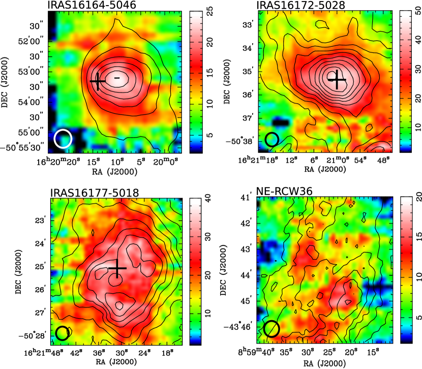
Figure 1: Integrated emission maps of ^13CO (contours) overlaid on [C i] of the four sources. The ^13CO contour levels start at 30 per cent of the peak integrated emission, with increments of $10\sigma$ for NE-RCW36, and $20\sigma$ for the other three sources. ^13CO peak integrated emission are 131, 189, 164 and 28 K km s^-1 for IRAS16164–5046, IRAS16172–5028, IRAS16177–5018 and NE-RCW36 respectively. $1\sigma$ level of ^13CO integrated emission maps are 0.7 K km s^-1 for IRAS16164–5046, IRAS16172–5028 and IRAS16177–5018, 0.3 K km s^-1 for NE-RCW36, $3\sigma$ level are outside the presented ^13CO maps. Color scales are clipped at $3\sigma$ level, where $1\sigma$ is 0.7 K km s^-1 for IRAS16164–5046 and IRAS16172-5028, 0.6 K km s^-1 for IRAS16177-5018 and NE-RCW36. Beam sizes are marked by circles. The crosses mark the location of the IRAS sources, except RCW36 which is outside the map.

To show the velocity structure of these regions, position-velocity (PV) diagrams of [C i] (grey scale) and ^13CO (contours) are plotted in Figure 2 (top row), with line profiles of [C i] and ^13CO averaged over the region in the integrated emission maps (Figure 1 bottom four). [C i] and ^13CO have similar velocity structure, in the form of centroid velocity, line widths, line wings/shoulders due to outflows and infall, as show in the Gaussian fitted parameters of the spectra (Table 1). As mentioned previously, the $-48$ km s^-1 component of IRAS16164–5046 is due to a different source outside the presented map; here the PV diagram shows that this emission is detached from the main source. NE-RCW36 PV diagram shows two separate velocity components, 4 and 7 km s^-1, which are also spatially separated. Since the column density calculation in this work is per spatial pixel, any spatially separable velocity structure does not affect the derivation of column density.

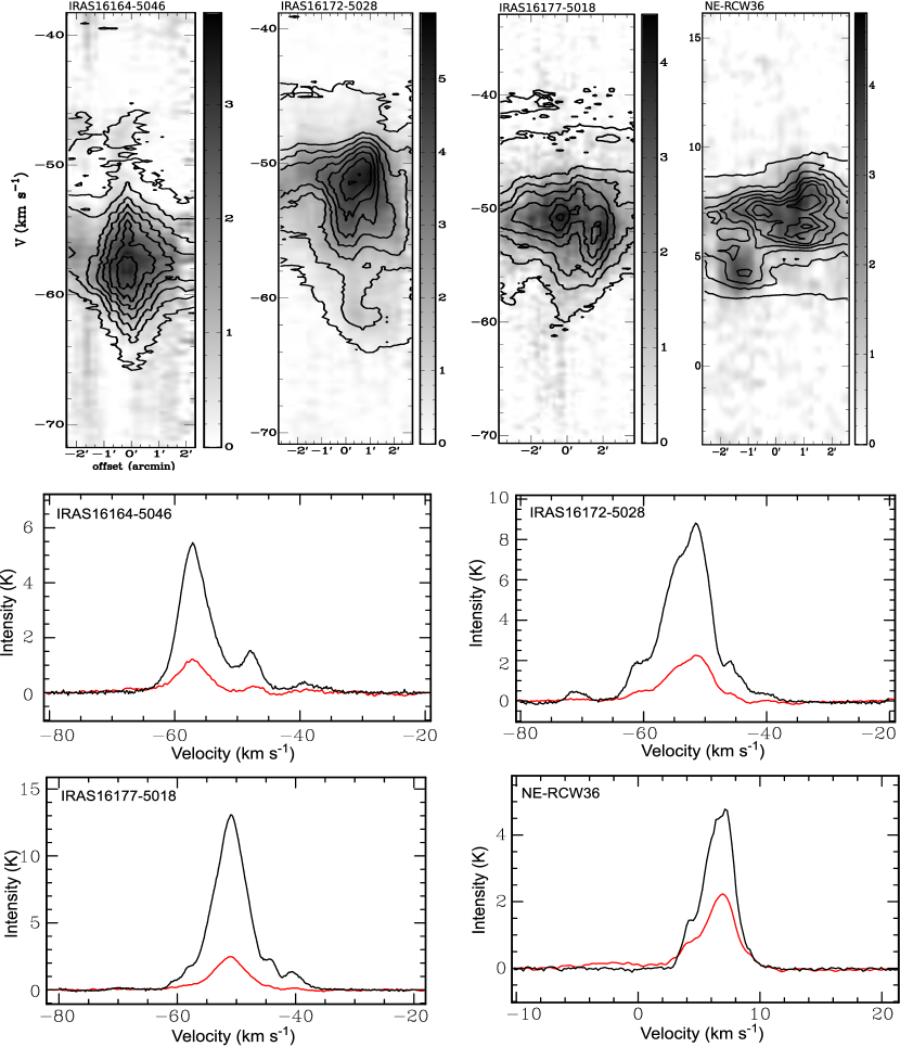
Figure 2: (Top row) [C i] and ^13CO (contours) position-velocity (PV). The contour levels start at $5\sigma$ noise level with increment of $10\sigma$, where $1\sigma$ is 0.2 K for IRAS16164–5046, 0.3 K for IRAS16172–5028 and IRAS16177–5018, and 0.1 K for NE-RCW36. PV cuts across each of the sources from NE to SW. (Line profiles) Averaged [C i] (red) and ^13CO (black) spectra over the area shown in Figure 1.

^13CO generally appears to be more extensive than [C i] as shown in Figure 1. However, we have determined that this is due the greater prevalence of artifacts in [C i] maps, compared with those of ^13CO maps. The noise in both ^13CO and [C i] maps is non-Gaussian, and is influenced in particular by fluctuations in weather at the times maps were taken. For [C i] at the higher frequency of 492 GHz, maps are more affected by poor weather than ^13CO transition at 110 GHz. As the artifacts/noise are non-Gaussian, it has not been possible to determine a specific contour level of ^13CO below which [C i] is no longer detected.

3.2 Column densities

The column density maps presented in this work is derived per spatial pixel, utilizing the integrated intensity maps in Section 3.1. H2 column density is obtained from the optically thick ^12CO, C i, and ^13CO column densities are corrected for opacity at each spatial pixel position.

For H2 column density, we utilize the empirical relation between H2 and ^12CO for Galactic molecular clouds (Shetty et al., 2011),

$$N_{\rm H_{2}}=2\times 10^{20}\int T_{\rm MB}{\rm(CO,J=1\to 0)}dV\,.$$ (1)

We follow the column density calculation outlined in Oka et al. (2001) for C i, which we repeat briefly here,

$$N_{\rm CI}=1.98\times 10^{15}\int T_{\rm MB}dV\,Q(T_{\rm ex})e^{E_{1}/(kT_{\rm ex})}\times\left[1-\frac{J_{\nu}(T_{\rm BB})}{J_{\nu}(T_{\rm ex})}\right]^{-1}\frac{\tau_{\rm CI}}{1-e^{-\tau_{\rm CI}}},$$ (2)

where $\int T_{\rm MB}dV$ is the integrated emission of [C i], $Q(T_{\rm ex})$ is the partition function,

$$Q(T_{\rm ex})=1+3{\rm e}^{E_{1}/(kT_{\rm ex})}+5{\rm e}^{E_{2}/(kT_{\rm ex})}\,,$$ (3)

with energy levels of $E_{1}/k=23.6$ K and $E_{2}/k=62.5$ K, $J_{\nu}(T_{\rm BB})$ and $J_{\nu}(T_{\rm ex})$ are the radiation temperature of cosmic background radiation ($T_{\rm BB}=2.7$ K) and excitation temperature ($T_{\rm ex}$) respectively, and $\tau_{\rm CI}$ is the opacity,

$$\tau_{\rm CI}=-{\rm ln}\left\{1-\frac{T_{\rm MB}}{\eta_{f}\left[J_{\nu}(T_{\rm ex})-J_{\nu}(T_{\rm BB})\right]}\right\}\,,$$ (4)

here we assume the beam filling factor $\eta_{f}=1$. Assuming C i has the same excitation temperature as the optically thick ^12CO at each of the spatial pixels, which is derived from the peak brightness temperature of ^12CO (Glover et al., 2014). We found the opacity of C i is between 0.1 to 1.3 across the maps. The total column density of C i is between $(0.1-8.4)\times 10^{17}$ cm^-2, where IRAS16172–5028 has the highest peak column density of $8.4\times 10^{17}$ cm^-2, and NE-RCW36 has the lowest peak column density of $3.3\times 10^{17}$ cm^-2.

For ^13CO column density, we corrected ^13CO opacity by assuming that C^18O is optically thin, and taking an isotopologue ratio of $\tau_{\rm 13CO}=7.4\tau_{\rm C18O}$ for the three sources in G333 GMC (Wong et al., 2008), and 5.5 for NE-RCW36. The opacity is then obtained by solving the brightness temperature-opacity relation,

$$\frac{T_{\rm 13CO}}{T_{\rm C18O}}=\frac{1-e^{-\tau_{\rm 13CO}}}{1-e^{-\tau_{\rm C18O}}}.$$ (5)

Similar to C i, we assume ^13CO has the same excitation temperature as ^12CO, the total column density of ^13CO is then,

$$N=\frac{8k\pi\nu^{2}}{hc^{3}g_{\rm u}A_{\rm ul}}\frac{\tau}{1-e^{-\tau}}e^{-E_{u}/(kT_{\rm ex})}Q(T_{\rm ex})\int T_{\rm b}dV\,,$$ (6)

where $\int T_{\rm b}dV$ is the integrated emission of ^13CO, upper energy level of $E_{u}/k=5.3$ K, $A_{\rm ul}$ is the Einstein $A$ coefficient in s^-1, transition frequency $\nu$ in Hz, the degeneracy $g_{u}$, and $Q(T_{\rm ex})$ is the partition function (Garden et al.,, 1991). We found the opacity of ^13CO to be between 0.1 and 5.3, and column density in the range of $(0.1-100)\times 10^{17}$ cm^-2. IRAS16172–5028 and IRAS16177–5018 have the highest peak column density ($\sim 10^{19}$ cm^-2), while similar to C i, NE-RCW36 has the lowest peak column density of $1.1\times 10^{18}$ cm^-2.

Simulation and modeling on how well C i traces molecular clouds suggest the $X_{\rm CI}-factor$ has a value of $1.1\times 10^{21}$ cm^-2 K^-1 km^-1 s, an analogue to the widely used $X_{\rm CO}-factor$ that connects integrated ^12CO emission to H2 column density (e.g. Offner et al., 2014; Glover et al., 2014). We apply this value to the integrated emission maps of [C i] to derive H2 column density ($N_{\rm H2-CI}$) and compare this to the H2 column density maps we obtained from ^12CO maps ($N_{\rm H2-CO}$). We note that the conversion factor is obtained from simulation and may not be fully applicable to the observed region here, due to variables such as local abundance, chemical and physical conditions. We found $N_{\rm H2-CI}$ traces 80 to 100 per cent of $N_{\rm H2-CO}$ for regions where ^13CO column density is between $\sim 5$ to $7\times 10^{18}$ cm^-2 and C i column density is between $\sim 4$ to $8\times 10^{17}$ cm^-2 for the three G333 IRAS sources, for NE-RCW36, the region is at $\sim 1\times 10^{17}$ cm^-2 for ^13CO and $\sim 2$ to $3\times 10^{17}$ cm^-2 for C i. A summary of the derived physical properties are listed in Table 1.

Table 1: Observational and physical parameters of the sources.

	IRAS16164–5046a	IRAS16172–5028b	IRAS16177–5018c	NE-RCW36d
Pointing centere ($\alpha,\delta$)	16 22.17, -50 06.1	16 21.06, -50 35.38	16 21.54, -50 25.33	08 59.43, -43 43.87
Parent Complex	G333	G333	G333	VMR-C
Distance	3.6 kpcf	3.6 kpcf	3.6 kpcf	0.7 kpcg
rms chan-1	0.4/0.3 K	0.3/0.3 K	0.3/0.3 K	0.3/0.2 K
(NANTEN2/Mopra)
$V_{\rm CI}$ (km s-1)h	$-47$, $-57$	$-45$, $-51$, $-54$, $-61$	$-45$, $-51$, $-58$	4.2, 7.0
$V_{\rm 13CO}$ (km s-1)h	$-48$, $-57$	$-45$, $-51$, $-54$, $-61$	$-40$, $-43$, $-50$, $-56$	4.2, 7.0
$\Delta V_{\rm CI}$ (km s-1)h	2.5, 5.9	1.7, 5.6, 6.2, 4.4	6.7, 6.0, 6.5	2.5, 2.7
$\Delta V_{\rm 13CO}$ (km s-1)h	5.9, 5.6	2.8, 4.2, 6.2, 3.1	4.2, 3.1, 6.0, 6.8	1.5, 2.6
$\tau_{\rm CI}$j	0.2 - 1.3 (0.5)	0.2 - 0.8 (0.3)	0.1 - 0.6 (0.3)	0.1 - 0.8 (0.3)
$\tau_{\rm 13CO}$j	0.9 - 5.3 (2.8)	0.1 - 5.3 (2.2)	0.1 - 4.3 (2.2)	0.04 - 3.0 (0.5)
$N_{\rm CI}$ ($\times 10^{17}$ cm-2)j	0.2 - 7 (2.2)	0.9 - 8 (2.9)	0.1 - 6 (2.6)	0.1 - 3 (1.3)
$N_{\rm 13CO}$ ($\times 10^{17}$ cm-2)j	3 - 59 (9.6)	0.3 - 99 (19)	0.5 - 100 (28)	0.1 - 11 (0.8)
$T_{\rm ex}$ (K)j	8 - 16 (12)	14 - 29 (19)j	17 - 29 (21)	12 - 34 (19)
$N_{\rm H2-CO}$ ($\times 10^{22}$ cm-2)k	0.5 - 2.2 (1.9)	2.4 - 6.6 (3.7)	2.8 - 5.6 (3.9)	0.7 - 2.1 (1.3)
$N_{\rm H2-CI}$ ($\times 10^{22}$ cm-2)k	0.3 - 2.6 (0.8)	1.1 - 5.1 (1.8)	0.8 - 4.1 (1.6)	0.3 - 1.9 (0.9)

4 Discussion

Recent C i mapping of the northern part of Orion-A GMC by Shimajiri et al. (2013) found a opacity of 0.1 - 0.75, similar to what we find (0.1 - 0.8) for three of our sources, with the exception of IRAS16164–5046 which reaches as high as 1.3 in optical depth at the [C i] emission peak. The highest C i column density in this work is of order of $\sim 10^{17}$ cm^-2, which is an order of magnitude lower than the peak value $\sim 10^{18}$ cm^-2 found in Orion-A. However, this could be due to effects such as resolution (i.e. beam filling factor less than 1). In fact, from modeling with the radiative transfer code RADEX (Van der Tak et al., 2007) for gas temperature shows $10^{18}$ cm^-2 fits our sources better (discussion later on).

We also find that the C i column density peak is offset from the peak H2 column density when the excitation temperature (both quantities derived from the peak ^12CO emission, Section 3.2) at the H2 peak column density exceeds 25 K (Figure 3). This is unlikely to be due to the optical thickness of ^12CO ‘shifting’ the apparent peak position, as from a cross check with the dust cores from ATLASGAL (Csengeri et al., 2014) and BLAST (Netterfield et al., 2009) data, their positions coincide well with the ^12CO peaks and thus the H2 column density peaks, except for source IRAS16177–5018, in which ^12CO is blended over various dust cores. In fact, at the peak C i column density position, $T_{\rm ex}$ is within 15 to 20 K. The only source (IRAS16164–5046) that has both the C i and H2 column density peaks coincide has an excitation temperature of $\sim 15$ K at this position. Furthermore, if we double the excitation temperature ($>30$ K) in C i column density calculations, it yields a lower column density at the C i peak position. Modeling of C i by Glover et al. (2014) shows around 80 per cent of C i is found in regions with temperature below 30 K, and from our observations, we also find C i is concentrated at places with lower excitation temperature (15 to 20 K). Depending on optical thickness, excitation temperature does not necessary equal gas kinetic temperature, and in the low opacity case, molecules are generally sub-thermally excited which makes the excitation temperature lower than kinetic temperature, so in either case, C i is found mainly in low temperature gas. One possible explanation for this is that the C i data presented here is from the observations of lower fine structure transition at 492 GHz with an energy level of 23 K. As the gas temperature rises, more of the neutral carbon atoms populate the higher transition level at 810 GHz with energy level of 62 K. To check whether this explanation is possible, we utilize the radiative transfer code RADEX by inputting gas temperatures in the range of 15 to 40 K. We find that as temperature rises, the intensity (population) of the 810 GHz transition increases from 2.8 to 20 K. Furthermore, the H2 column density we obtained with C i is comparable to H2 column density derived from ^12CO, in which ^12CO is an unreliable tracer at high density as it becomes optically thick (e.g. Shetty et al., 2011), and thus under estimates the column density. Despite that, the comparable H2 column density is suggesting that a portion of the neutral carbon atoms in the ${}^{3}P_{1}-^{3}P_{0}$ state appear to be missing. If this is the case, and if a substantial amount of atomic carbon is in an energy state above the ground state, we should see a position offset of the 810 GHz [C i] transition for the sources here, and follow up observations in the future will further investigate this. More importantly, observations of both [C i] transitions maybe necessary to recover the total C i gas.

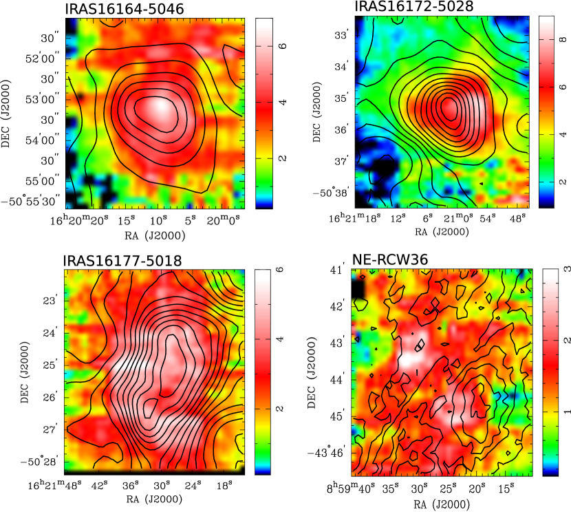
Figure 3: H2 column density map (contours) overlaid on C i column density map (color) of the four sources. The column density maps are at scale of $10^{21}$ cm^-2 and $10^{17}$ cm^-2 for H2 and C i. The H2 contour levels start at 40 per cent of peak column density (Table 1), except for IRAS16177–5018 which start at 50 per cent, the lowest visible contour level in the presented map. Contour steps are at 20$\sigma$, where 1$\sigma$ is $1\times 10^{20}$ cm^-2 for IRAS16164–5046, IRAS16177–5018 and NE-RCW36, and $1.5\times 10^{20}$ for IRAS16172-5028.

One possible uncertainty in our column density calculation comes from the velocity range in the integrated intensity maps. As shown in Section 3.1 these sources are not quiescent gases, they are turbulent with outflows (line wings). In order to access the effect of integrating over different gas components on column density derivation, two sets of velocity range are used: (1) integration over a velocity range that includes line wings/shoulders, (2) integration over the line width of the main core velocity component. In method (1), the H2 column density derived from [C i] is comparable to those derived from ^12CO (Table 1). With method (2), H2 column density obtained from [C i] is approximately 10 to 30 per cent higher than those from ^12CO, but still within an order of magnitude. However, by integrating over the line width only can be problematic with ^12CO, as it is self-absorbed at the core velocity component, and the application of $X-factor$ requires ^12CO being optically thick and an integration over the emission range. Given the H2 column density derived from ^12CO and [C i] in both methods are comparable and within the same order of magnitude, the choice of velocity range does not alter the conclusion in this work.

Another uncertainty in deriving H2 column density is the value of $X_{\rm CI}-factor$, unlike CO, the relationship between [C i] intensity and H2 column density is not well studied. The value we used in this work is from simulation studies (Offner et al., 2014; Glover et al., 2014), not specifically calibrated for the presented regions. The simulations do not take into account active star formation, where strong UV radiation increases the abundance of C i, and thus, altering the value of $X_{\rm CI}-factor$. There is no observational/simulation study on $X_{\rm CI}-factor$ among active star forming regions (at the time of this work), but if star formation raises the abundance of C i, then the $X_{\rm CI}-factor$ would be higher in these cases, and thus increases the derived H2 column density. We are in the process of completing the C i mapping, along with various molecular lines at 3 mm wavelengths, we can calibrate the $X-factor$ of C i and other molecules (e.g. HCO+, CS, HCN) by comparing the H2 density estimated from SED fits of continuum emissions.

5 Conclusion

We present the first results of C i mapping of VMR-C and G333 GMCs, comparing the column density of H2 derived from both C i and CO isotopologues. The [C i] emission profile is similar to ^13CO with comparable line widths. We found C i has opacity between 0.1 to 1.3, column density of $(0.1-8)\times 10^{17}$ cm^-2, an order of magnitude lower than ^13CO column density. Utilizing the $X_{\rm CI}-factor$ we found an H2 column density of order $\sim 10^{22}$ cm^-2, which is within the same order of magnitude of H2 column density derived from ^12CO, and near 100 per cent at [C i] peak emission location. [C i] emission tends to peak at regions with low gas temperature ($<20$ K), and it yields the same H2 column density as those derived from ^12CO at this temperature range. This could be due to part of the carbon atoms are in a higher excitation state, further mapping of C i transition at 810 GHz will help confirm this.

Our results suggest if the gas is warm (above 25 K), it is recommended to observe both of the [C i] transitions for a more accurate determination of H2 column density. C i has the advantage of low opacity compared to ^12CO, while in low density and low extinction regions CO is dissociated into neutral carbon and oxygen, making C i a better tracer in these cases. However, in regions of dense gas where local abundance of ^13CO is known, ^13CO may be a better choice for probing H2 column density, as it is easily observed due to the lower frequency of its emission lines.

References

- Bains et al. (2006) Bains, I., Wong, T., Cunningham, M. R. et al., 2006, MNRAS, 367, 1609
- Batchelor et al. (1980) Batchelor R. A., Caswell J. L., Haynes R. F. et al. 1980, AuJPh, 33, 139
- Becklin et al. (1973) Becklin E. E., Frogel J. A., Neugebauer G. et al., 1973, ApJ, 182, L125
- Breen et al. (2007) Breen, S. L., Ellingsen, S. P., Johnston-Hollitt, M. et al., 2007, MNRAS, 377, 491-506
- Caswell et al. (1995) Caswell J. L., Vaile R. A., Ellingsen S. P. et al., 1995, MNRAS, 272, 96
- Caswell (1998) Caswell J. L., 1998, MNRAS, 297, 215
- Csengeri et al. (2014) Csengeri, T., Urquhart, J. S., Schuller, F. et al., 2014, A&A, 565, 75
- Figueredo et al., (2005) Figuerêdo, E., Blum, R. D., Damineli, A. et al., 2005, AJ, 129, 1523-1533
- Fujiyoshi et al. (2006) Fujiyoshi T., Smith C. H., Caswell J. L. et al., 2006, MNRAS, 368, 1843
- Garden et al., (1991) Garden, R. P., Hayashi, M., Hasegawa, T. et al., 1991, ApJ, 374, 540
- Glover et al. (2014) Glover, S. C. O., Clark, P. C., Micic, M., Molina, F., 2014, MNRAS, submitted, arXiv:1403.3530
- Grave et al. (2014) Grave J. M. C., Kumar M. S. N., Ojha D. K. et al., 2014, A&A, 563, AA123
- Ladd et al. (2005) Ladd, N., Purcell, C., Wong, T. & Robertson, S. 2005, PASA, 22, 62
- Lo et al. (2007) Lo, N., Cunningham, M., Bains, I. et al., 2007, MNRAS, 381, L30-L34
- Lo et al. (2009) Lo, N., Cunningham, M. R., Jones, P. A. et al., 2009, MNRAS, 395, 1021
- Lockman (1979) Lockman F. J., 1979, ApJ, 232, 761
- Minier et al. (2013) Minier V., Tremblin, P., Hill, T. et al., 2013, A&A, 550, AA50
- Mookerjea et al. (2004) Mookerjea, B., Kramer, C., Nielbock, M., Nyman, L.-Å., 2004, A&A, 426, 119
- Murphy & May (1991) Murphy, D. C., May, J., 1991, A&A, 247, 202-214
- Netterfield et al. (2009) Netterfield, C. B., Ade, P. A. R., Bock, J. J., 2009, ApJ, 707, 1824
- Offner et al. (2014) Offner, S. S. R., Bisbas, T. G., Bell, T. A., Viti, S., 2014, MNRAS, 440, 81
- Oka et al. (2001) Oka, T., Yamamoto, S., Iwata, M. et al., 2001, ApJ, 558, 176
- Roman-Lopes et al. (2009) Roman-Lopes, A., Abraham, Z., Ortiz, R., & Rodriguez-Ardila, A. 2009, MNRAS, 394, 467
- Shetty et al. (2011) Shetty, R., Glover, S. C., Dullemond, C. P., Klessen, R. S., 2011, MNRAS, 412, 1686
- Shimajiri et al. (2013) Shimajiri, Y., Sakai, T., Tsukagoshi, T. et al., 2013, ApJL, 774, L20
- Van der Tak et al. (2007) Van der Tak, F.F.S., Black, J.H., Schöier, F.L., Jansen, D.J., van Dishoeck, E.F., 2007, A&A, 468, 627
- Wong et al. (2008) Wong, T., Ladd, E. F., Brisbin, D. et al., 2008, MNRAS, 386, 1069
- Yamaguchi et al. (1999) Yamaguchi, N., Mizuno, N., Saito, H. et al., 1999, PASJ, 51, 775