Equilibrated tractions for the Hybrid High-Order method

Abstract

We show how to recover equilibrated face tractions for the hybrid high-order method for linear elasticity recently introduced in [1], and prove that these tractions are optimally convergent.

Résumé Tractions équilibrées pour la méthode hybride d’ordre élevé. Nous montrons comment obtenir des tractions de face équilibrées pour la méthode hybride d’ordre élevé pour l’élasticité linéaire rrécemment introduite dans [1] et prouvons que ces tractions convergent de manière optimale.

1 Introduction

Let $\Omega\subset\mathbb{R}^{d}$, $d\in\{2,3\}$, denote a bounded connected polygonal or polyhedral domain. For $X\subset\overline{\Omega}$, we denote by $(\cdot,\cdot)_{X}$ and $\|{\cdot}\|_{X}$ respectively the standard inner product and norm of $L^{2}(X)$, and a similar notation is used for $L^{2}(X)^{d}$ and $L^{2}(X)^{d\times d}$. For a given external load $\vec{f}\in L^{2}(\Omega)^{d}$, we consider the linear elasticity problem: Find $\vec{u}\in H_{0}^{1}(\Omega)^{d}$ such that

$$2\mu(\boldsymbol{\nabla}_{\rm s}\vec{u},\boldsymbol{\nabla}_{\rm s}\vec{v})_{\Omega}+\lambda(\boldsymbol{\nabla}{\cdot}\vec{u},\boldsymbol{\nabla}{\cdot}\vec{v})_{\Omega}=(\vec{f},\vec{v})_{\Omega}.$$ (1)

with $\mu>0$ and $\lambda\geq 0$ real numbers representing the scalar Lamé coefficients and $\boldsymbol{\nabla}_{\rm s}$ denoting the symmetric gradient operator. Classically, the solution to (1) satisfies $-\boldsymbol{\nabla}{\cdot}\matr{\sigma}(\vec{u})=\vec{f}$ a.e. in $\Omega$ with stress tensor $\matr{\sigma}(\vec{u})\mathrel{\mathop{:}}=2\mu\boldsymbol{\nabla}_{\rm s}\vec{u}+\lambda\matr{I}_{d}(\boldsymbol{\nabla}{\cdot}\vec{u})$. Denoting by $T$ an open subset of $\Omega$ with non-zero Hausdorff measure ($T$ will represent a mesh element in what follows), partial integration yields the following local equilibrium property:

$$(\matr{\sigma}(\vec{u}),\boldsymbol{\nabla}_{\rm s}\vec{\mathsf{v}}_{T})_{T}-(\matr{\sigma}(\vec{u})\vec{n}_{T},\vec{\mathsf{v}}_{T})_{\partial T}=(\vec{f},\vec{\mathsf{v}}_{T})_{T}\qquad\forall\vec{\mathsf{v}}_{T}\in\mathbb{P}_{d}^{k}(T)^{d},$$ (2)

where $\partial T$ and $\vec{n}_{T}$ denote, respectively, the boundary and outward normal to $T$. Additionally, the normal interface tractions $\matr{\sigma}(\vec{u})\vec{n}_{T}$ are equilibrated across $\partial T\cap\Omega$. The goal of this work is to (i) devise a reformulation of the Hybrid High-Order method for linear elasticity introduced in [1] that identifies its local equilibrium properties expressed by a discrete counterpart of (2) and (ii) to show how the corresponding equilibrated face tractions can be obtained by element-wise post-processing. This is an important complement to the original analysis, as local equilibrium is an essential property in practice. The material is organized as follows: in Section 2 we outline the original formulation of the HHO method; in Section 3 we derive the local equilibrium formulation based on a new local displacement reconstruction.

2 The Hybrid High-Order method

We consider admissible mesh sequences in the sense of [2, Section 1.4]. Each mesh $\mathcal{T}_{h}$ in the sequence is a finite collection $\{T\}$ of nonempty, disjoint, open, polytopic elements such that $\overline{\Omega}=\bigcup_{T\in\mathcal{T}_{h}}\overline{T}$ and $h=\max_{T\in\mathcal{T}_{h}}h_{T}$ (with $h_{T}$ the diameter of $T$), and there is a matching simplicial submesh of $\mathcal{T}_{h}$ with locally equivalent mesh size and which is shape-regular in the usual sense. For all $T\in\mathcal{T}_{h}$, the faces of $T$ are collected in the set $\mathcal{F}_{T}$ and, for all $F\in\mathcal{F}_{T}$, $\vec{n}_{TF}$ is the unit normal to $F$ pointing out of $T$. Additionally, interfaces are collected in the set $\mathcal{F}_{h}^{{\rm i}}$ and boundary faces in $\mathcal{F}_{h}^{{\rm b}}$. The diameter of a face $F\in\mathcal{F}_{h}$ is denoted by $h_{F}$. For the sake of brevity, we abbreviate $a\lesssim b$ the inequality $a\leq Cb$ for positive real numbers $a$ and $b$ and a generic constant $C$ which can depend on the mesh regularity, on $\mu$, $d$, and the polynomial degree, but is independent of $h$ and $\lambda$. We also introduce the notation $a\simeq b$ for the uniform equivalence $a\lesssim b\lesssim a$.

Let a polynomial degree $k\geq 1$ be fixed. The local and global spaces of degrees of freedom (DOFs) are

$$\underline{\vec{\mathsf{U}}}_{T}^{k}\mathrel{\mathop{:}}=\mathbb{P}_{d}^{k}(T)^{d}\times\left\{\bigtimes_{F\in\mathcal{F}_{T}}\mathbb{P}_{d-1}^{k}(F)^{d}\right\}\quad\forall T\in\mathcal{T}_{h},\qquad\underline{\vec{\mathsf{U}}}_{h}^{k}\mathrel{\mathop{:}}=\left\{\bigtimes_{T\in\mathcal{T}_{h}}\mathbb{P}_{d}^{k}(T)^{d}\right\}\times\left\{\bigtimes_{F\in\mathcal{F}_{h}}\mathbb{P}_{d-1}^{k}(F)^{d}\right\}.$$ (3)

A generic collection of DOFs from $\underline{\vec{\mathsf{U}}}_{h}^{k}$ is denoted by $\underline{\vec{\mathsf{v}}}_{h}=\big{(}(\vec{\mathsf{v}}_{T})_{T\in\mathcal{T}_{h}},(\vec{\mathsf{v}}_{F})_{F\in\mathcal{F}_{h}}\big{)}$ and, for a given $T\in\mathcal{T}_{h}$, $\underline{\vec{\mathsf{v}}}_{T}=\big{(}\vec{\mathsf{v}}_{T},(\vec{\mathsf{v}}_{F})_{F\in\mathcal{F}_{T}}\big{)}\in\underline{\vec{\mathsf{U}}}_{T}^{k}$ indicates its restriction to $\underline{\vec{\mathsf{U}}}_{T}^{k}$. For all $T\in\mathcal{T}_{h}$, we define a high-order local displacement reconstruction operator $\vec{p}_{T}^{k}:\underline{\vec{\mathsf{U}}}_{T}^{k}\to\mathbb{P}_{d}^{k+1}(T)^{d}$ by solving the following (well-posed) pure traction problem: For a given $\underline{\vec{\mathsf{v}}}_{T}\in\underline{\vec{\mathsf{U}}}_{T}^{k}$, $\vec{p}_{T}^{k}\underline{\vec{\mathsf{v}}}_{T}$ is such that

$$(\boldsymbol{\nabla}_{\rm s}\vec{p}_{T}^{k}\underline{\vec{\mathsf{v}}}_{T},\boldsymbol{\nabla}_{\rm s}\vec{w})_{T}=(\boldsymbol{\nabla}_{\rm s}\vec{\mathsf{v}}_{T},\boldsymbol{\nabla}_{\rm s}\vec{w})_{T}+\sum_{F\in\mathcal{F}_{T}}(\vec{\mathsf{v}}_{F}-\vec{\mathsf{v}}_{T},\boldsymbol{\nabla}_{\rm s}\vec{w}\,\vec{n}_{TF})_{F}\qquad\forall\vec{w}\in\mathbb{P}_{d}^{k+1}(T)^{d},$$ (4)

and the rigid-body motion components of $\vec{p}_{T}^{k}\underline{\vec{\mathsf{v}}}_{T}$ are prescribed so that $\int_{T}\vec{p}_{T}^{k}\underline{\vec{\mathsf{v}}}_{T}=\int_{T}\vec{\mathsf{v}}_{T}$ and $\int_{T}\boldsymbol{\nabla}_{\rm ss}(\vec{p}_{T}^{k}\underline{\vec{\mathsf{v}}}_{T})=\sum_{F\in\mathcal{F}_{T}}\int_{F}\frac{1}{2}(\vec{n}_{TF}{\otimes}\vec{\mathsf{v}}_{F}-\vec{\mathsf{v}}_{F}{\otimes}\vec{n}_{TF})$ where $\boldsymbol{\nabla}_{\rm ss}$ is the skew-symmetric gradient operator. Additionally, we define the divergence reconstruction $D_{T}^{k}:\underline{\vec{\mathsf{U}}}_{T}^{k}\to\mathbb{P}_{d}^{k}(T)$ such that, for a given $\underline{\vec{\mathsf{v}}}_{T}\in\underline{\vec{\mathsf{U}}}_{T}^{k}$,

$$(D_{T}^{k}\underline{\vec{\mathsf{v}}}_{T},q)_{T}=(\boldsymbol{\nabla}{\cdot}\vec{\mathsf{v}}_{T},q)_{T}+\sum_{F\in\mathcal{F}_{T}}(\vec{\mathsf{v}}_{F}-\vec{\mathsf{v}}_{T},q\vec{n}_{TF})_{F}\qquad\forall q\in\mathbb{P}_{d}^{k}(T).$$ (5)

We introduce the local bilinear form $a_{T}:\underline{\vec{\mathsf{U}}}_{T}^{k}\times\underline{\vec{\mathsf{U}}}_{T}^{k}\to\mathbb{R}$ such that

$$a_{T}(\underline{\vec{\mathsf{w}}}_{T},\underline{\vec{\mathsf{v}}}_{T})\mathrel{\mathop{:}}=2\mu\left\{(\boldsymbol{\nabla}_{\rm s}\vec{p}_{T}^{k}\underline{\vec{\mathsf{w}}}_{T},\boldsymbol{\nabla}_{\rm s}\vec{p}_{T}^{k}\underline{\vec{\mathsf{v}}}_{T})_{T}+s_{T}(\underline{\vec{\mathsf{w}}}_{T},\underline{\vec{\mathsf{v}}}_{T})\right\}+\lambda(D_{T}^{k}\underline{\vec{\mathsf{w}}}_{T},D_{T}^{k}\underline{\vec{\mathsf{v}}}_{T})_{T},$$ (6)

where the stabilizing bilinear form $s_{T}:\underline{\vec{\mathsf{U}}}_{T}^{k}\times\underline{\vec{\mathsf{U}}}_{T}^{k}\to\mathbb{R}$ is such that

$$s_{T}(\underline{\vec{\mathsf{w}}}_{T},\underline{\vec{\mathsf{v}}}_{T})\mathrel{\mathop{:}}=\sum_{F\in\mathcal{F}_{T}}h_{F}^{-1}(\pi_{F}^{k}(\vec{P}_{T}^{k}\underline{\vec{\mathsf{w}}}_{T}-\vec{\mathsf{w}}_{F}),\pi_{F}^{k}(\vec{P}_{T}^{k}\underline{\vec{\mathsf{v}}}_{T}-\vec{\mathsf{v}}_{F}))_{F},$$ (7)

and a second displacement reconstruction $\vec{P}_{T}^{k}:\underline{\vec{\mathsf{U}}}_{T}^{k}\to\mathbb{P}_{d}^{k+1}(T)$ is defined such that, for all $\underline{\vec{\mathsf{v}}}_{T}\in\underline{\vec{\mathsf{U}}}_{T}^{k}$, $\vec{P}_{T}^{k}\underline{\vec{\mathsf{v}}}_{T}\mathrel{\mathop{:}}=\vec{\mathsf{v}}_{T}+(\vec{p}_{T}^{k}\underline{\vec{\mathsf{v}}}_{T}-\pi_{T}^{k}\vec{p}_{T}^{k}).$ Let $\underline{\vec{I}}_{T}^{k}:H^{1}(T)^{d}\to\underline{\vec{\mathsf{U}}}_{T}^{k}$ be the reduction map such that, for all $T\in\mathcal{T}_{h}$ and all $\vec{v}\in H^{1}(T)^{d}$, $\underline{\vec{I}}_{T}^{k}\vec{v}=\big{(}\pi_{T}^{k}\vec{v},(\pi_{F}^{k}\vec{v})_{F\in\mathcal{F}_{T}}\big{)}$. The potential reconstruction $\vec{p}_{T}^{k}$ and the bilinear form $s_{T}$ are conceived so that they satisfy the following two key properties:

1. Stability. For all $\underline{\vec{\mathsf{v}}}_{T}\in\underline{\vec{\mathsf{U}}}_{T}^{k}$,

   $$\|\boldsymbol{\nabla}_{\rm s}\vec{p}_{T}^{k}\underline{\vec{\mathsf{v}}}_{T}\|_{T}^{2}+s_{T}(\underline{\vec{\mathsf{v}}}_{T},\underline{\vec{\mathsf{v}}}_{T})\simeq\|\boldsymbol{\nabla}_{\rm s}\vec{\mathsf{v}}_{T}\|_{T}^{2}+j_{T}(\underline{\vec{\mathsf{v}}}_{T},\underline{\vec{\mathsf{v}}}_{T}),$$ (8)

   with bilinear form $j_{T}:\underline{\vec{\mathsf{U}}}_{T}^{k}\times\underline{\vec{\mathsf{U}}}_{T}^{k}\to\mathbb{R}$ such that $j_{T}(\underline{\vec{\mathsf{w}}}_{T},\underline{\vec{\mathsf{v}}}_{T})\mathrel{\mathop{:}}=\sum_{F\in\mathcal{F}_{T}}h_{F}^{-1}(\vec{\mathsf{w}}_{T}-\vec{\mathsf{w}}_{F},\vec{\mathsf{v}}_{T}-\vec{\mathsf{v}}_{F})_{F}.$

2. Approximation. For all $\vec{v}\in H^{k+2}(T)^{d}$,

   $$\big{\{}\|\boldsymbol{\nabla}_{\rm s}(\vec{v}-\vec{p}_{T}^{k}\underline{\vec{I}}_{T}^{k}\vec{v})\|_{T}^{2}+s_{T}(\underline{\vec{I}}_{T}^{k}\vec{v},\underline{\vec{I}}_{T}^{k}\vec{v})\big{\}}^{\nicefrac{{1}}{{2}}}\lesssim h_{T}^{k+1}\|\vec{v}\|_{H^{k+2}(T)^{d}}.$$ (9)

We observe that, unlike $s_{T}$, the stabilization bilinear form $j_{T}$ only satisfies $j_{T}(\underline{\vec{I}}_{T}^{k}\vec{v},\underline{\vec{I}}_{T}^{k}\vec{v})\lesssim h^{k}\|\vec{v}\|_{H^{k+1}(T)^{d}}$. The discrete problem reads: Find $\underline{\vec{\mathsf{u}}}_{h}\in\underline{\vec{\mathsf{U}}}_{h,0}^{k}\mathrel{\mathop{:}}=\{\underline{\vec{\mathsf{u}}}_{h}\in\underline{\vec{\mathsf{U}}}_{h}^{k}\;|\;\vec{\mathsf{u}}_{F}\equiv\vec{0}\quad\forall F\in\mathcal{F}_{h}^{{\rm b}}\}$ such that

$$a_{h}(\underline{\vec{\mathsf{u}}}_{h},\underline{\vec{\mathsf{v}}}_{h})\mathrel{\mathop{:}}=\sum_{T\in\mathcal{T}_{h}}a_{T}(\underline{\vec{\mathsf{w}}}_{T},\underline{\vec{\mathsf{v}}}_{T})=\sum_{T\in\mathcal{T}_{h}}(\vec{f},\vec{\mathsf{v}}_{T})_{T}\qquad\forall\underline{\vec{\mathsf{v}}}_{h}\in\underline{\vec{\mathsf{U}}}_{h,0}^{k}.$$ (10)

The following convergence result was proved in [1]:

Theorem 1 (Energy error estimate).

Let $\vec{u}\in H_{0}^{1}(\Omega)^{d}$ and $\underline{\vec{\mathsf{u}}}_{h}\in\underline{\vec{\mathsf{U}}}_{h,0}^{k}$ denote the unique solutions to (1) and (10), respectively, and assume $\vec{u}\in H^{k+2}(\Omega)^{d}$ and $\boldsymbol{\nabla}{\cdot}\vec{u}\in H^{k+1}(\Omega)$. Then, letting $\underline{\vec{\widehat{\mathsf{u}}}}_{h}\in\underline{\vec{\mathsf{U}}}_{h,0}^{k}$ be such that $\underline{\vec{\widehat{\mathsf{u}}}}_{T}\mathrel{\mathop{:}}=\underline{\vec{I}}_{T}^{k}\vec{u}$ for all $T\in\mathcal{T}_{h}$, the following holds (with $\|\underline{\vec{\mathsf{v}}}_{T}\|_{a,T}^{2}=a_{T}(\underline{\vec{\mathsf{v}}}_{T},\underline{\vec{\mathsf{v}}}_{T})$ for all $\underline{\vec{\mathsf{v}}}_{T}\in\underline{\vec{\mathsf{U}}}_{T}^{k}$):

$$\sum_{T\in\mathcal{T}_{h}}\|\underline{\vec{\mathsf{u}}}_{T}-\underline{\vec{\widehat{\mathsf{u}}}}_{T}\|_{a,T}^{2}\lesssim h^{2(k+1)}\left(\|\vec{u}\|_{H^{k+2}(\Omega)^{d}}+\lambda\|\boldsymbol{\nabla}{\cdot}\vec{u}\|_{H^{k+1}(\Omega)}\right)^{2}.$$ (11)

Moreover, assuming elliptic regularity, $\sum_{T\in\mathcal{T}_{h}}\|\vec{u}-\vec{p}_{T}^{k}\underline{\vec{\mathsf{u}}}_{T}\|_{L^{2}(T)^{d}}^{2}\lesssim h^{2(k+2)}\left(\|\vec{u}\|_{H^{k+2}(\Omega)^{d}}+\lambda\|\boldsymbol{\nabla}{\cdot}\vec{u}\|_{H^{k+1}(\Omega)}\right)^{2}$.

3 Local equilibrium formulation

The difficulty in devising an equivalent local equilibrium formulation for problem (10) comes from the stabilization term $s_{T}$, which introduces a non-trivial coupling of interface DOFs inside each element. In this section, we introduce post-processed discrete displacement and stress reconstructions that allow us to circumvent this difficulty. For a given element $T\in\mathcal{T}_{h}$, define the following bilinear form on $\underline{\vec{\mathsf{U}}}_{T}^{k}$:

$$\widetilde{a}_{T}(\underline{\vec{\mathsf{w}}}_{T},\underline{\vec{\mathsf{v}}}_{T})\mathrel{\mathop{:}}=2\mu\left\{(\boldsymbol{\nabla}_{\rm s}\vec{p}_{T}^{k}\underline{\vec{\mathsf{w}}}_{T},\boldsymbol{\nabla}_{\rm s}\vec{p}_{T}^{k}\underline{\vec{\mathsf{v}}}_{T})_{T}+j_{T}(\underline{\vec{\mathsf{w}}}_{T},\underline{\vec{\mathsf{v}}}_{T})\right\}+\lambda(D_{T}^{k}\underline{\vec{\mathsf{w}}}_{T},D_{T}^{k}\underline{\vec{\mathsf{v}}}_{T})_{T},$$ (12)

where the only difference with respect to the bilinear form $a_{T}$ defined by (6) is that we have stabilized using $j_{T}$ instead of $s_{T}$. We observe that, while proving a discrete local equilibrium relation for the method based on $\widetilde{a}_{T}$ would not require any local post-processing, the suboptimal consistency properties of $j_{T}$ would only yield $h^{2k}$ in the right-hand side of (11). Denoting by $\|{\cdot}\|_{\widetilde{a},T}$ the local seminorm induced by $\widetilde{a}_{T}$ on $\underline{\vec{\mathsf{U}}}_{T}^{k}$, one can prove that, for all $\underline{\vec{\mathsf{v}}}_{T}\in\underline{\vec{\mathsf{U}}}_{T}^{k}$,

$$\|\underline{\vec{\mathsf{v}}}_{T}\|_{\widetilde{a},T}\simeq\|\underline{\vec{\mathsf{v}}}_{T}\|_{a,T}.$$ (13)

We next define the isomorphism $\underline{\vec{\mathsf{c}}}_{T}^{k}:\underline{\vec{\mathsf{U}}}_{T}^{k}\to\underline{\vec{\mathsf{U}}}_{T}^{k}$ such that

$$\widetilde{a}_{T}(\underline{\vec{\mathsf{c}}}_{T}^{k}\underline{\vec{\mathsf{w}}}_{T},\underline{\vec{\mathsf{v}}}_{T})=a_{T}(\underline{\vec{\mathsf{w}}}_{T},\underline{\vec{\mathsf{v}}}_{T})+(2\mu)j_{T}(\underline{\vec{\mathsf{w}}}_{T},\underline{\vec{\mathsf{v}}}_{T})\qquad\forall\underline{\vec{\mathsf{v}}}_{T}\in\underline{\vec{\mathsf{U}}}_{T}^{k},$$ (14)

and rigid-body motion components prescribed as above. We also introduce the stress reconstruction $\matr{S}_{T}^{k}:\underline{\vec{\mathsf{U}}}_{T}^{k}\to\mathbb{P}_{d}^{k}(T)^{d\times d}$ such that

$$\matr{S}_{T}^{k}\mathrel{\mathop{:}}=(2\mu\boldsymbol{\nabla}_{\rm s}\vec{p}_{T}^{k}+\lambda\matr{I}_{d}D_{T}^{k})\circ\underline{\vec{\mathsf{c}}}_{T}^{k}.$$ (15)

Lemma 2 (Equilibrium formulation).

The bilinear form $a_{T}$ defined by (6) is such that, for all $\underline{\vec{\mathsf{w}}}_{T},\underline{\vec{\mathsf{v}}}_{T}\in\underline{\vec{\mathsf{U}}}_{T}^{k}$,

$$a_{T}(\underline{\vec{\mathsf{w}}}_{T},\underline{\vec{\mathsf{v}}}_{T})=(\matr{S}_{T}^{k}\underline{\vec{\mathsf{w}}}_{T},\boldsymbol{\nabla}_{\rm s}\vec{\mathsf{v}}_{T})_{T}+\sum_{F\in\mathcal{F}_{T}}(\vec{\tau}_{TF}(\underline{\vec{\mathsf{w}}}_{T}),\vec{\mathsf{v}}_{F}-\vec{\mathsf{v}}_{T})_{F},$$ (16)

with interface traction $\vec{\tau}_{TF}:\underline{\vec{\mathsf{U}}}_{T}^{k}\to\mathbb{P}_{d-1}^{k}(F)^{d}$ such that

$$\vec{\tau}_{TF}(\underline{\vec{\mathsf{w}}}_{T})=\matr{S}_{T}^{k}\underline{\vec{\mathsf{w}}}_{T}\,\vec{n}_{TF}+h_{F}^{-1}\left[\big{(}(\underline{\vec{\mathsf{c}}}_{T}^{k}\underline{\vec{\mathsf{w}}}_{T})_{F}-\vec{\mathsf{w}}_{F}\big{)}-\big{(}(\underline{\vec{\mathsf{c}}}_{T}^{k}\underline{\vec{\mathsf{w}}}_{T})_{T}-\vec{\mathsf{w}}_{T}\big{)}\right].$$ (17)

Proof.

Let $\underline{\vec{\widetilde{\mathsf{w}}}}_{T}\mathrel{\mathop{:}}=\underline{\vec{\mathsf{c}}}_{T}^{k}\underline{\vec{\mathsf{w}}}_{T}$. We have, using the definitions (14) of $\underline{\vec{\mathsf{c}}}_{T}^{k}$ and (12) of the bilinear form $\widetilde{a}_{T}$,

$$a_{T}(\underline{\vec{\mathsf{w}}}_{T},\underline{\vec{\mathsf{v}}}_{T}) =\widetilde{a}_{T}(\underline{\vec{\widetilde{\mathsf{w}}}}_{T},\underline{\vec{\mathsf{v}}}_{T})-(2\mu)j_{T}(\underline{\vec{\mathsf{w}}}_{T},\underline{\vec{\mathsf{v}}}_{T})$$

$$=2\mu\left\{(\boldsymbol{\nabla}_{\rm s}\vec{p}_{T}^{k}\underline{\vec{\widetilde{\mathsf{w}}}}_{T},\boldsymbol{\nabla}_{\rm s}\vec{p}_{T}^{k}\underline{\vec{\mathsf{v}}}_{T})_{T}+j_{T}(\underline{\vec{\widetilde{\mathsf{w}}}}_{T}-\underline{\vec{\mathsf{w}}}_{T},\underline{\vec{\mathsf{v}}}_{T})\right\}+\lambda(D_{T}^{k}\underline{\vec{\widetilde{\mathsf{w}}}}_{T},D_{T}^{k}\underline{\vec{\mathsf{v}}}_{T})_{T}$$

$$=(\matr{S}_{T}^{k}\underline{\vec{\mathsf{w}}}_{T},\boldsymbol{\nabla}_{\rm s}\vec{\mathsf{v}}_{T})_{T}+\sum_{F\in\mathcal{F}_{T}}(\matr{S}_{T}^{k}\underline{\vec{\mathsf{w}}}_{T}\,\vec{n}_{TF},\vec{\mathsf{v}}_{F}-\vec{\mathsf{v}}_{T})_{F}+(2\mu)j_{T}(\underline{\vec{\widetilde{\mathsf{w}}}}_{T}-\underline{\vec{\mathsf{w}}}_{T},\underline{\vec{\mathsf{v}}}_{T}),$$

where we have concluded using (4) with $\vec{w}=\vec{p}_{T}^{k}\underline{\vec{\widetilde{\mathsf{w}}}}_{T}$, (5) with $q=D_{T}^{k}\underline{\vec{\widetilde{\mathsf{w}}}}_{T}$, and recalling the definition (15) of $\matr{S}_{T}^{k}$. To obtain (16), it suffices to use the definition of $j_{T}$. ∎

Lemma 3 (Local equilibrium).

Let $\underline{\vec{\mathsf{u}}}_{h}\in\underline{\vec{\mathsf{U}}}_{h,0}^{k}$ denote the unique solution to (10). Then, for all $T\in\mathcal{T}_{h}$, the following discrete counterpart of the local equilibrium relation (2) holds:

$$(\matr{S}_{T}^{k}\underline{\vec{\mathsf{u}}}_{T},\boldsymbol{\nabla}_{\rm s}\vec{\mathsf{v}}_{T})_{T}-\sum_{F\in\mathcal{F}_{T}}(\vec{\tau}_{TF}(\underline{\vec{\mathsf{u}}}_{T}),\vec{\mathsf{v}}_{T})_{F}=(\vec{f},\vec{\mathsf{v}}_{T})_{T}\qquad\forall\vec{\mathsf{v}}_{T}\in\mathbb{P}_{d}^{k}(T)^{d},$$ (18)

and the numerical flux are equilibrated in the following sense: For all $F\in\mathcal{F}_{h}^{{\rm i}}$ such that $F\subset\partial T_{1}\cap\partial T_{2}$,

$$\vec{\tau}_{T_{1}F}(\underline{\vec{\mathsf{u}}}_{T_{1}})+\vec{\tau}_{T_{1}F}(\underline{\vec{\mathsf{u}}}_{T_{2}})=\vec{0}.$$ (19)

Proof.

To prove (18), let an element $T\in\mathcal{T}_{h}$ be fixed, take as an ansatz collection of DOFs in (10) $\underline{\vec{\mathsf{v}}}_{h}=\big{(}(\vec{\mathsf{v}}_{T})_{T\in\mathcal{T}_{h}},(\vec{0})_{F\in\mathcal{F}_{h}}\big{)}$ with $\vec{\mathsf{v}}_{T}$ in $\mathbb{P}_{d}^{k}(T)^{d}$ and $\vec{\mathsf{v}}_{T^{\prime}}\equiv\vec{0}$ for all $T^{\prime}\in\mathcal{T}_{h}\setminus\{T\}$, and use (16) with $\underline{\vec{\mathsf{w}}}_{T}=\underline{\vec{\mathsf{u}}}_{T}$ to conclude that $a_{T}(\underline{\vec{\mathsf{u}}}_{T},\underline{\vec{\mathsf{v}}}_{T})$ corresponds to the left-hand side of (18). Similarly, to prove (19), let an interface $F\in\mathcal{F}_{h}^{{\rm i}}$ be fixed and take as an ansatz collection of DOFs in (10) $\underline{\vec{\mathsf{v}}}_{h}=\big{(}(\vec{0})_{T\in\mathcal{T}_{h}},(\vec{\mathsf{v}}_{F})_{F\in\mathcal{F}_{h}}\big{)}\in\underline{\vec{\mathsf{U}}}_{h,0}^{k}$ with $\vec{\mathsf{v}}_{F}$ in $\mathbb{P}_{d-1}^{k}(F)^{d}$ and $\vec{\mathsf{v}}_{F^{\prime}}\equiv\vec{0}$ for all $F^{\prime}\in\mathcal{F}_{h}\setminus\{F\}$. Then, using (16) with $\underline{\vec{\mathsf{w}}}_{T}=\underline{\vec{\mathsf{u}}}_{T}$ in (10), it is inferred that $a_{h}(\underline{\vec{\mathsf{u}}}_{h},\underline{\vec{\mathsf{v}}}_{h})=(\vec{\tau}_{T_{1}F}(\underline{\vec{\mathsf{u}}}_{T_{1}})+\vec{\tau}_{T_{2},F}(\underline{\vec{\mathsf{u}}}_{T_{2}}),\vec{\mathsf{v}}_{F})_{F}=0,$ which proves the desired result since $\vec{\tau}_{T_{1}F}(\underline{\vec{\mathsf{u}}}_{T_{1}})+\vec{\tau}_{T_{2}F}(\underline{\vec{\mathsf{u}}}_{T_{2}})\in\mathbb{P}_{d-1}^{k}(F)^{d}$. ∎

To conclude, we show that the locally post-processed solution yields a new collection of DOFs that is an equally good approximation of the exact solution as is the discrete solution $\underline{\vec{\mathsf{u}}}_{h}$. Consequently, the equilibrated face numerical tractions defined in (17) optimally converge to the exact tractions.

Proposition 4 (Convergence for $\underline{\vec{\mathsf{c}}}_{T}^{k}\underline{\vec{\mathsf{u}}}_{T}$).

Using the notation of Theorem 1, the following holds:

$$\sum_{T\in\mathcal{T}_{h}}\|\underline{\vec{\mathsf{c}}}_{T}^{k}\underline{\vec{\mathsf{u}}}_{T}-\underline{\vec{\widehat{\mathsf{u}}}}_{T}\|_{a,T}^{2}\lesssim h^{2(k+1)}\left(\|\vec{u}\|_{H^{k+2}(\Omega)^{d}}+\lambda\|\boldsymbol{\nabla}{\cdot}\vec{u}\|_{H^{k+1}(\Omega)}\right)^{2}.$$ (20)

Proof.

Let $T\in\mathcal{T}_{h}$. Recalling (14), we have

$$\widetilde{a}_{T}(\underline{\vec{\mathsf{c}}}_{T}^{k}\underline{\vec{\mathsf{u}}}_{T}-\underline{\vec{\widehat{\mathsf{u}}}}_{T},\underline{\vec{\mathsf{v}}}_{T}) =a_{T}(\underline{\vec{\mathsf{u}}}_{T},\underline{\vec{\mathsf{v}}}_{T})+(2\mu)j_{T}(\underline{\vec{\mathsf{u}}}_{T},\underline{\vec{\mathsf{v}}}_{T})-\widetilde{a}_{T}(\underline{\vec{\widehat{\mathsf{u}}}}_{T},\underline{\vec{\mathsf{v}}}_{T})$$

$$=a_{T}(\underline{\vec{\mathsf{u}}}_{T}-\underline{\vec{\widehat{\mathsf{u}}}}_{T},\underline{\vec{\mathsf{v}}}_{T})+(2\mu)s_{T}(\underline{\vec{\widehat{\mathsf{u}}}}_{T},\underline{\vec{\mathsf{v}}}_{T})+(2\mu)j_{T}(\underline{\vec{\mathsf{u}}}_{T}-\underline{\vec{\widehat{\mathsf{u}}}}_{T},\underline{\vec{\mathsf{v}}}_{T}).$$

Hence, using the Cauchy–Schwarz inequality followed by the stability property (8) and multiple applications of the norm equivalence (13),

$$|\widetilde{a}_{T}(\underline{\vec{\mathsf{c}}}_{T}^{k}\underline{\vec{\mathsf{u}}}_{T}-\underline{\vec{\widehat{\mathsf{u}}}}_{T},\underline{\vec{\mathsf{v}}}_{T})| \leq\left\{\|\underline{\vec{\mathsf{u}}}_{T}-\underline{\vec{\widehat{\mathsf{u}}}}_{T}\|_{a,T}^{2}+(2\mu)s_{T}(\underline{\vec{\widehat{\mathsf{u}}}}_{T},\underline{\vec{\widehat{\mathsf{u}}}}_{T})+(2\mu)j_{T}(\underline{\vec{\mathsf{u}}}_{T}-\underline{\vec{\widehat{\mathsf{u}}}}_{T},\underline{\vec{\mathsf{u}}}_{T}-\underline{\vec{\widehat{\mathsf{u}}}}_{T})\right\}^{\nicefrac{{1}}{{2}}}\|\underline{\vec{\mathsf{v}}}_{T}\|_{\widetilde{a},T}$$

$$\lesssim\left\{\|\underline{\vec{\mathsf{u}}}_{T}-\underline{\vec{\widehat{\mathsf{u}}}}_{T}\|_{a,T}^{2}+(2\mu)s_{T}(\underline{\vec{\widehat{\mathsf{u}}}}_{T},\underline{\vec{\widehat{\mathsf{u}}}}_{T})\right\}^{\nicefrac{{1}}{{2}}}\|\underline{\vec{\mathsf{v}}}_{T}\|_{\widetilde{a},T}.$$

Using again (13) followed by the latter inequality, we infer that

$$\|\underline{\vec{\mathsf{c}}}_{T}^{k}\underline{\vec{\mathsf{u}}}_{T}-\underline{\vec{\widehat{\mathsf{u}}}}_{T}\|_{a,T}\lesssim\|\underline{\vec{\mathsf{c}}}_{T}^{k}\underline{\vec{\mathsf{u}}}_{T}-\underline{\vec{\widehat{\mathsf{u}}}}_{T}\|_{\widetilde{a},T}={\sup_{\underline{\vec{\mathsf{v}}}_{T}\in\underline{\vec{\mathsf{U}}}_{T}^{k}\setminus\{\mathsf{\vec{0}}\}}}\frac{\widetilde{a}_{T}(\underline{\vec{\mathsf{c}}}_{T}^{k}\underline{\vec{\mathsf{u}}}_{T}-\underline{\vec{\widehat{\mathsf{u}}}}_{T},\underline{\vec{\mathsf{v}}}_{T})}{\|\underline{\vec{\mathsf{v}}}_{T}\|_{\widetilde{a},T}}\lesssim\left\{\|\underline{\vec{\mathsf{u}}}_{T}-\underline{\vec{\widehat{\mathsf{u}}}}_{T}\|_{a,T}^{2}+(2\mu)s_{T}(\underline{\vec{\widehat{\mathsf{u}}}}_{T},\underline{\vec{\widehat{\mathsf{u}}}}_{T})\right\}^{\nicefrac{{1}}{{2}}}.$$

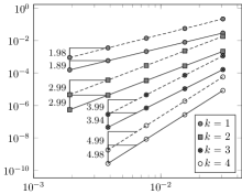
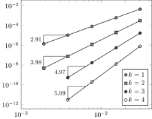
Figure 1: Convergence results in the energy-norm (left) and $L^{2}$-norm (right) for the solution to (10) (solid lines) and its post-processing based on $\underline{\vec{\mathsf{c}}}_{T}^{k}$ (dashed lines). The right panel shows that the post-processing has no sizable effect on element unknowns.

The estimate (20) then follows squaring the above inequality, summing over $T\in\mathcal{T}_{h}$, and using (11) and (9), respectively, to bound the terms in the right-hand side. ∎

To assess the estimate (20), we have numerically solved the pure displacement problem with exact solution $\vec{u}=\big{(}\sin(\pi x_{1})\sin(\pi x_{2})+\nicefrac{{1}}{{2}}x_{1},\cos(\pi x_{1})\cos(\pi x_{2})+\nicefrac{{1}}{{2}}x_{2}\big{)}$ for $\mu=\lambda=1$ on a $h$-refined sequence of triangular meshes. The corresponding convergence results are presented in Figure 1. In the left panel, we compare the quantities on the left-hand side of estimates (11) and (20). Although the order of convergence is the same, the original solution $\underline{\vec{\mathsf{u}}}_{h}$ displays better accuracy in the energy-norm. This is essentially due to face unknowns, as confirmed in the right panel, where the square roots of the quantities $\sum_{T\in\mathcal{T}_{h}}\|\vec{\mathsf{u}}_{T}-\vec{\widehat{\mathsf{u}}}_{T}\|_{T}^{2}$ and $\sum_{T\in\mathcal{T}_{h}}\|\underline{\vec{\mathsf{c}}}_{T}^{k}\underline{\vec{\mathsf{u}}}_{T}-\vec{\widehat{\mathsf{u}}}_{T}\|_{T}^{2}$ (both of which are discrete $L^{2}$-norms of the error) are plotted.

References

• [1] D. A. Di Pietro, A. Ern, A hybrid high-order locking-free method for linear elasticity on general meshes, Comput. Meth. Appl. Mech. Engrg. 283 (2015) 1–21.
• [2] D. A. Di Pietro, A. Ern, Mathematical aspects of discontinuous Galerkin methods, Vol. 69 of Mathématiques & Applications, Springer-Verlag, Berlin, 2012.