Prior Support Knowledge-Aided Sparse Bayesian Learning with Partly Erroneous Support Information

Abstract

It has been shown both experimentally and theoretically that sparse signal recovery can be significantly improved given that part of the signal’s support is known a priori. In practice, however, such prior knowledge is usually inaccurate and contains errors. Using such knowledge may result in severe performance degradation or even recovery failure. In this paper, we study the problem of sparse signal recovery when partial but partly erroneous prior knowledge of the signal’s support is available. Based on the conventional sparse Bayesian learning framework, we propose a modified two-layer Gaussian-inverse Gamma hierarchical prior model and, moreover, an improved three-layer hierarchical prior model. The modified two-layer model employs an individual parameter $b_{i}$ for each sparsity-controlling hyperparameter $\alpha_{i}$, and has the ability to place non-sparsity-encouraging priors to those coefficients that are believed in the support set. The three-layer hierarchical model is built on the modified two-layer prior model, with a prior placed on the parameters $\{b_{i}\}$ in the third layer. Such a model enables to automatically learn the true support from partly erroneous information through learning the values of the parameters $\{b_{i}\}$. Variational Bayesian algorithms are developed based on the proposed hierarchical prior models. Numerical results are provided to illustrate the performance of the proposed algorithms.

I Introduction

Compressed sensing is a recently emerged technique for signal sampling and data acquisition which enables to recover sparse signals from much fewer linear measurements [1, 2, 3, 4, 5]. In this paper, we study the problem of sparse signal recovery when prior information on the signal’s partial support is available. In practice, prior information about the support region of the sparse signal may come from the support estimate obtained during a previous time instant. This is particularly the case for time-varying sparse signals whose support changes slowly over time. For example, in the real-time dynamic magnetic resonance imaging (MRI) reconstruction, it was shown that the support of a medical image sequence undergoes small variations with support changes (number of additions and removals) less than $2\%$ of the support size [6]. Also, in the source localization problem, the locations of sources may vary slowly over time. Thus the previous estimate of locations can be used as prior knowledge to enhance the accuracy of the current estimate.

The problem of sparse signal recovery with partial support information was studied in several independent and parallel works [7, 6, 8, 9]. In [7], the partly known support is utilized to obtain a least-squares residual and compressed sensing is then performed on the least-squares residual instead of the original observation. When the partly known support is accurate, it is expected that the sparse signal associated with the residual has much fewer large nonzero components. Hence the least-squares residual-based compressed sensing can improve the recovery performance. Later in [6], a weighted $\ell_{1}$-minimization (modified basis pursuit) method was proposed, where the partially known support is excluded from the $\ell_{1}$-minimization (equivalent to setting the corresponding weights to zero). Sufficient conditions for exact reconstruction were derived, and it was shown that when a fairly accurate estimate of the true support is available, the exact reconstruction conditions are much weaker than the sufficient conditions for compressed sensing without utilizing the prior information [6]. This work was later extended to the noisy case [10], where a regularized modified basis pursuit denoising method was introduced and a computable bound on the reconstruction error was obtained. The weighted $\ell_{1}$-minimization approach was also studied in [8] by assuming a probabilistic support model which assigns a probability of being zero or nonzero to each entry of the sparse signal. The choice of the weights and the associated exact recovery conditions were investigated. In [9], a modified iterative reweighted method which incorporates the prior support information was proposed. Similar to [6], those weights corresponding to the a priori known support are assigned a very small value (close to zero), whereas other weights are recursively updated like conventional iterative reweighted methods. The problem of support knowledge-aided sparse signal recovery was also studied in a time-varying compressed sensing framework, e.g. [11, 12], where the temporal support correlation was modeled by a Markov chain [11] or a pattern-coupled structure [12]. Nevertheless, both works need to specify the inherent support correlation structure between two consecutive time steps, whereas our work here deals with a more general scenario involving no particular correlation structure between the prior support and the current support.

It has been observed [7, 6, 8, 9] that the sparse recovery performance can be significantly improved through exploiting the prior support knowledge. Nevertheless, this improvement can only be achieved when the prior knowledge is fairly accurate. Existing methods, e.g. [7, 6, 8, 9], may suffer from severe recovery performance degradation or even recovery failure in the presence of inaccurate prior knowledge. In practice, however, signal support estimation inevitably incurs errors, and in some cases, due to the support variation across time, the prior knowledge may contain a considerable amount of errors. In this paper, we first introduce a modified two-layer Gaussian-inverse Gamma prior model, where an individual parameter $b_{i}$, instead of a common parameter $b$ used in the conventional framework, is employed to characterize each sparsity-controlling hyperparameter $\alpha_{i}$. Through assigning different values to the parameters $\{b_{i}\}$, our new prior model has the flexibility to place non-sparsity-encouraging priors to those coefficients that are believed in the support set. Nevertheless, the above modified two-layer hierarchical model does not have a mechanism to learn the true support from the partly erroneous knowledge. To address this issue, we propose an improved hierarchical prior model which constitutes a three-layer hierarchical form, where a new layer is proposed in addition to the above modified two-layer hierarchical model. The new layer places a prior on the parameters $\{b_{i}\}$. Such an approach is capable of distinguishing the true support from erroneous support through learning the values of $\{b_{i}\}$. By resorting to the variational inference methodology, we develop a new sparse Bayesian learning method which has the ability to learn the true support from the erroneous information.

The rest of the paper is organized as follows. In Section II, we introduce a modified two-layer Gaussian-inverse Gamma hierarchical prior model and an improved three-layer hierarchical prior model which enables to learn the true support from partly erroneous knowledge. Variational Bayesian methods are developed in Section III. Simulation results are provided in Section IV, followed by concluding remarks in Section V.

II Hierarchical Prior Model

We consider the problem of recovering a sparse signal $\boldsymbol{x}\in\mathbb{R}^{n}$ from noise-corrupted measurements

$$\boldsymbol{y}=\boldsymbol{A}\boldsymbol{x}+\boldsymbol{w}$$ (1)

where $\boldsymbol{A}\in\mathbb{R}^{m\times n}$ ($m<n$) is the measurement matrix, and $\boldsymbol{w}$ is the additive multivariate Gaussian noise with zero mean and covariance matrix $\sigma^{2}\boldsymbol{I}$. Suppose we have partial but partly erroneous knowledge of the support of the sparse signal $\boldsymbol{x}$. The prior knowledge $P$ can be divided into two parts: $P=S\cup E$, where $S$ denotes the subset containing correct information and $E$ denotes the error subset. If we let $T$ denote the true support of $\boldsymbol{x}$ and $T^{c}$ denote the complement of the set $T$, i.e. $T\cup T^{c}=\{1,2,\ldots,n\}$, then we have $S\subset T$, and $E\subset T^{c}$. Note that the only prior information we have is $P$. The partition of $S$ and $E$ is unknown to us.

The prior support information can certainly be utilized to improve signal recovery. In the following, based on the conventional sparse Bayesian learning (SBL) framework, we first introduce a modified SBL hierarchical prior model which has the flexibility to place non-sparsity-encouraging priors to those coefficients that are believed in the support set. Furthermore, we propose an improved three-layer hierarchical prior model which enables to learn the true support from the erroneous information and thus exploits the prior support information in a more constructive manner. To facilitate discussions and comparisons, we first provide a brief overview of the conventional SBL hierarchical model.

II-A Overview of Conventional SBL

Sparse Bayesian learning was originally developed by Tipping in [13] to address regression and classification problems. Later on in [14, 15, 16, 17], sparse Bayesian learning was adapted to solve the sparse recovery problem and obtained superior performance for sparse signal recovery in a series of experiments. In the conventional sparse Bayesian learning framework, a two-layer hierarchical prior model was proposed to promote the sparsity of the solution. In the first layer, $\boldsymbol{x}$ is assigned a Gaussian prior distribution

$$p(\boldsymbol{x}|\boldsymbol{\alpha})=\prod_{i=1}^{n}p(x_{i}|\alpha_{i})$$ (2)

where $p(x_{i}|\alpha_{i})=\mathcal{N}(x_{i}|0,\alpha_{i}^{-1})$, and $\boldsymbol{\alpha}\triangleq\{\alpha_{i}\}$, the inverse variance (precision) of the Gaussian distribution, are non-negative sparsity-controlling hyperparameters. The second layer specifies Gamma distributions as hyperpriors over the hyperparameters $\{\alpha_{i}\}$, i.e.

$$p(\boldsymbol{\alpha})=\prod_{i=1}^{n}\text{Gamma}(\alpha_{i}|a,b)=\prod_{i=1}^{n}\Gamma(a)^{-1}b^{a}\alpha_{i}^{a-1}e^{-b\alpha_{i}}$$ (3)

where $\Gamma(a)=\int_{0}^{\infty}t^{a-1}e^{-t}dt$ is the Gamma function, the parameters $a$ and $b$ used to characterize the Gamma distribution are chosen to be very small values, e.g. $10^{-4}$, in order to provide non-informative/uniform (over a logarithmic scale) hyperpriors over $\{\alpha_{i}\}$. As discussed in [13], a broad hyperprior allows the posterior mean of $\alpha_{i}$ to become arbitrarily large. As a consequence, the associated coefficient $x_{i}$ will be driven to zero, thus yielding a sparse solution. This mechanism is also referred to as the “automatic relevance determination” mechanism which tends to switch off most of the coefficients that are deemed to be irrelevant, and only keep very few relevant coefficients to explain the data.

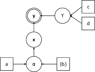
(a) A modified two-layer hierarchical prior model

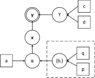
(b) A three-layer hierarchical prior model.

Figure 1: Hierarchical models for support knowledge-aided sparse Bayesian learning.

II-B Modified Two-Layer Hierarchical Model

When the value of the parameter $b$ is relatively large, e.g. $b=0.5$, it can be readily observed from (3) that the hyperpriors are no longer uniform and now they encourage small values of $\{\alpha_{i}\}$. In this case, an arbitrarily large value of the posterior mean of $\alpha_{i}$ is prohibited. As a result, the two-layer hierarchical model no longer results in a sparsity-encouraging prior and therefore does not necessarily lead to a sparse solution. This fact inspires us to develop a new way to incorporate the prior support information into the sparse Bayesian learning framework. Specifically, instead of using a common parameter $b$ for all sparsity-controlling hyperparameters $\{\alpha_{i}\}$, we hereby employ an individual parameter $b_{i}$ for each hyperparameter $\alpha_{i}$, i.e.

$$p(\boldsymbol{\alpha})=\prod_{i=1}^{n}\text{Gamma}(\alpha_{i}|a,b_{i})=\prod_{i=1}^{n}\Gamma(a)^{-1}b_{i}^{a}\alpha_{i}^{a-1}e^{-b_{i}\alpha_{i}}$$ (4)

Such a formulation allows us to assign different priors to different coefficients. If the partial knowledge of the signal’s support, $P$, is available, then the associated parameters of $\{b_{i}\}$ can be set to a relatively large value, say $0.5$, in order to place a non-sparsity-encouraging prior on the corresponding coefficients, whereas the rest parameters of $\{b_{i}\}$ are still assigned a small value, say $10^{-4}$, to encourage sparse coefficients, that is,

$$b_{i}=\begin{cases}0.5&i\in P\\ 10^{-4}&i\in P^{c}\end{cases}$$ (5)

where $P^{c}$ denotes the complement of $P$, i.e. $P\cup P^{c}=\{1,2\ldots,n\}$. The above modified hierarchical model seamlessly integrates the prior support information into the sparse Bayesian learning framework. Nevertheless, the modified two-layer hierarchical model which assigns fixed values to $\{b_{i}\}$ still lacks the flexibility to learn and adapt to the true situation. When the prior information contains a considerable portion of errors, this approach may suffer from significant performance loss and even recovery failure.

II-C Proposed Three-Layer Hierarchical Model

To address the above issue, we partition the parameters $\{b_{i}\}$ into two subsets: $\{b_{i},\forall i\in P\}$, and $\{b_{i},\forall i\in P^{c}\}$. For $\{b_{i},\forall i\in P^{c}\}$, the parameters are still considered to be deterministic and assigned a very small value, e.g. $10^{-4}$; while for $\{b_{i},\forall i\in P\}$, instead of assigning a fixed large value, we model them as random parameters and place hyperpriors over these parameters. Since $\{b_{i},\forall i\in P\}$ are positive values, suitable priors over $\{b_{i},\forall i\in P\}$ are also Gamma distributions. In summary, we have

$$p(b_{i})=\begin{cases}\text{Gamma}(b_{i}|p,q)=\Gamma(p)^{-1}q^{p}b_{i}^{p-1}e^{-qb_{i}}&i\in P\\ \delta(b_{i}-10^{-4})&i\in P^{c}\end{cases}$$ (6)

where $\delta(\cdot)$ denotes the Dirac delta function, $p$ and $q$ are parameters characterizing the Gamma distribution and their choice will be discussed in Section III. We see that the proposed model constitutes a three-layer hierarchical form which allows to learn the parameters $\{b_{i},\forall i\in P\}$ in an automatic manner from the data. The proposed algorithm based on this prior model therefore has the ability to identify the correct support from erroneous information.

III Variational Bayesian Inference

We now proceed to perform variational Bayesian inference for the proposed hierarchical models. Throughout this paper, the noise variance $\sigma^{2}$ is assumed unknown, and needs to be estimated along with other parameters. For notational convenience, define

$$\gamma\triangleq\sigma^{-2}$$

Following the conventional sparse Bayesian learning framework [13], we place a Gamma hyperprior over $\gamma$:

$$p(\gamma)=\text{Gamma}(\gamma|c,d)=\Gamma(c)^{-1}d^{c}\gamma^{c-1}e^{-d\gamma}$$ (7)

where the parameters $c$ and $d$ are set to small values, e.g. $c=d=10^{-4}$. Before proceeding, we firstly provide a brief review of the variational Bayesian methodology.

III-A Review of The Variational Bayesian Methodology

In a probabilistic model, let $\boldsymbol{y}$ and $\boldsymbol{\theta}$ denote the observed data and the hidden variables, respectively. It is straightforward to show that the marginal probability of the observed data can be decomposed into two terms

$$\ln p(\boldsymbol{y})=L(q)+\text{KL}(q||p)$$ (8)

where

$$L(q)=\int q(\boldsymbol{\theta})\ln\frac{p(\boldsymbol{y},\boldsymbol{\theta})}{q(\boldsymbol{\theta})}d\boldsymbol{\theta}$$ (9)

and

$$\text{KL}(q||p)=-\int q(\boldsymbol{\theta})\ln\frac{p(\boldsymbol{\theta}|\boldsymbol{y})}{q(\boldsymbol{\theta})}d\boldsymbol{\theta}$$ (10)

where $q(\boldsymbol{\theta})$ is any probability density function, $\text{KL}(q||p)$ is the Kullback-Leibler divergence between $p(\boldsymbol{\theta}|\boldsymbol{y})$ and $q(\boldsymbol{\theta})$. Since $\text{KL}(q||p)\geq 0$, it follows that $L(q)$ is a rigorous lower bound on $\ln p(\boldsymbol{y})$. Moreover, notice that the left hand side of (8) is independent of $q(\boldsymbol{\theta})$. Therefore maximizing $L(q)$ is equivalent to minimizing $\text{KL}(q||p)$, and thus the posterior distribution $p(\boldsymbol{\theta}|\boldsymbol{y})$ can be approximated by $q(\boldsymbol{\theta})$ through maximizing $L(q)$.

The significance of the above transformation is that it circumvents the difficulty of computing the posterior probability $p(\boldsymbol{\theta}|\boldsymbol{y})$ directly (which is usually computationally intractable). For a suitable choice for the distribution $q(\boldsymbol{\theta})$, the quantity $L(q)$ may be more amiable to compute. Specifically, we could assume some specific parameterized functional form for $q$ and then maximize $L(q)$ with respect to the parameters of the distribution. A particular form of $q(\boldsymbol{\theta})$ that has been widely used with great success is the factorized form over the component variables $\{\theta_{i}\}$ in $\boldsymbol{\theta}$, i.e.

$$q(\boldsymbol{\theta})=\prod_{i}q_{i}(\theta_{i})$$ (11)

We therefore can compute the posterior distribution approximation by finding $q(\boldsymbol{\theta})$ of the form (11) that maximizes the lower bound $L(q)$. The maximization can be conducted in an alternating fashion for each latent variable, which leads to [18]

$$q_{i}(\theta_{i})=\frac{\exp(\langle\ln p(\boldsymbol{y},\boldsymbol{\theta})\rangle_{k\neq i})}{\int\exp(\langle\ln p(\boldsymbol{y},\boldsymbol{\theta})\rangle_{k\neq i})d\theta_{i}}$$ (12)

where $\langle\cdot\rangle_{k\neq i}$ denotes an expectation with respect to the distributions $q(\theta_{i})$ for all $k\neq i$.

III-B Bayesian Inference for Modified Two-Layer Model

Let $\boldsymbol{\theta}\triangleq\{\boldsymbol{x},\boldsymbol{\alpha},\boldsymbol{\gamma}\}$ denote all hidden variables. We assume posterior independence among the variables $\boldsymbol{x}$, $\boldsymbol{\alpha}$, and $\gamma$, i.e.

$$p(\boldsymbol{\theta}|\boldsymbol{y})\approx q(\boldsymbol{x},\boldsymbol{\alpha},\gamma)$$

$$= q_{x}(\boldsymbol{x})q_{\alpha}(\boldsymbol{\alpha})q_{\gamma}(\gamma)$$ (13)

With this mean field approximation, the posterior distribution of each hidden variable can be computed by maximizing $L(q)$ while keeping other variables fixed using their most recent distributions, which gives

$$\ln q_{x}(\boldsymbol{x})= \langle\ln p(\boldsymbol{y},\boldsymbol{x},\boldsymbol{\alpha},\gamma)\rangle_{q_{\alpha}(\boldsymbol{\alpha})q_{\gamma}(\gamma)}+\text{constant}$$

$$\ln q_{\alpha}(\boldsymbol{\alpha})= \langle\ln p(\boldsymbol{y},\boldsymbol{x},\boldsymbol{\alpha},\gamma)\rangle_{q_{x}(\boldsymbol{x})q_{\gamma}(\gamma)}+\text{constant}$$

$$\ln q_{\gamma}(\gamma)= \langle\ln p(\boldsymbol{y},\boldsymbol{x},\boldsymbol{\alpha},\gamma)\rangle_{q_{x}(\boldsymbol{x})q_{\alpha}(\boldsymbol{\alpha})}+\text{constant}$$

where $\langle\rangle_{q(\cdot)}$ denotes the expectation with respect to (w.r.t.) the distribution $q(\cdot)$. In summary, the posterior distribution approximations are computed in an alternating fashion for each hidden variable, with other variables fixed. Details of this Bayesian inference scheme are provided below.

1). Update of $q_{x}(\boldsymbol{x})$: Keeping only the terms that depend on $\boldsymbol{x}$, the variational optimization of $q_{x}(\boldsymbol{x})$ yields

$$\ln q_{x}(\boldsymbol{x})\propto \langle\ln p(\boldsymbol{y}|\boldsymbol{x},\gamma)+\ln p(\boldsymbol{x}|\boldsymbol{\alpha})\rangle_{q_{\alpha}(\boldsymbol{\alpha})q_{\gamma}(\gamma)}$$

$$\propto -\frac{\langle\gamma\rangle}{2}(\boldsymbol{y}-\boldsymbol{A}\boldsymbol{x})^{T}(\boldsymbol{y}-\boldsymbol{A}\boldsymbol{x})-\frac{1}{2}\boldsymbol{x}^{T}\langle\boldsymbol{D}\rangle\boldsymbol{x}$$ (14)

where $\langle\gamma\rangle$ denotes the expectation w.r.t. $q_{\gamma}(\gamma)$, and $\langle\boldsymbol{D}\rangle\triangleq\text{diag}(\langle\alpha_{1}\rangle,\ldots,\langle\alpha_{n}\rangle)$, in which $\langle\alpha_{i}\rangle$ represents the expectation w.r.t. $q_{\alpha}(\alpha)$. It can be readily verified that $q_{x}(\boldsymbol{x})$ follows a Gaussian distribution with its mean $\boldsymbol{\mu}$ and covariance matrix $\boldsymbol{\Phi}$ given respectively as

$$\boldsymbol{\mu}= \langle\gamma\rangle\boldsymbol{\Phi}\boldsymbol{A}^{T}\boldsymbol{y}$$

$$\boldsymbol{\Phi}= \left(\langle\gamma\rangle\boldsymbol{A}^{T}\boldsymbol{A}+\langle\boldsymbol{D}\rangle\right)^{-1}$$ (15)

2). Update of $q_{\alpha}(\boldsymbol{\alpha})$: Similarly, the approximate posterior $q_{\alpha}(\boldsymbol{\alpha})$ can be obtained by computing

$$\ln q_{\alpha}(\boldsymbol{\alpha})\propto \langle\ln p(\boldsymbol{x}|\boldsymbol{\alpha})+\ln p(\boldsymbol{\alpha}|a,\boldsymbol{b})\rangle_{q_{x}(\boldsymbol{x})}$$

$$\propto \sum_{i=1}^{n}\left\{\left(a-\frac{1}{2}\right)\ln\alpha_{i}-\left(b_{i}+\frac{\langle x_{i}^{2}\rangle}{2}\right)\alpha_{i}\right\}$$ (16)

where $\langle x_{i}^{2}\rangle$ denotes the expectation w.r.t. $q_{x}(\boldsymbol{x})$. Thus $\boldsymbol{\alpha}$ has a form of a product of Gamma distributions

$$q_{\alpha}(\boldsymbol{\alpha})=\prod_{i=1}^{n}\text{Gamma}(\alpha_{i};\tilde{a},\tilde{b}_{i})$$ (17)

in which the parameters $\tilde{a}$ and $\tilde{b}_{i}$ are respectively given as

$$\tilde{a}=a+\frac{1}{2}\qquad\tilde{b}_{i}=b+\frac{1}{2}\langle x_{i}^{2}\rangle$$ (18)

3). Update of $q_{\gamma}(\boldsymbol{\gamma})$: The approximate posterior distribution $q_{\gamma}(\boldsymbol{\gamma})$ can be computed as

$$\ln q_{\gamma}(\boldsymbol{\gamma})\propto \langle\ln p(\boldsymbol{y}|\boldsymbol{x},\gamma)+\ln p(\gamma|c,d)\rangle_{q_{x}(\boldsymbol{x})}$$

$$\propto \left(\frac{m}{2}+c\right)\ln\gamma$$

$$-\left(\frac{1}{2}\langle(\boldsymbol{y}-\boldsymbol{A}\boldsymbol{x})^{T}(\boldsymbol{y}-\boldsymbol{A}\boldsymbol{x})\rangle_{q_{x}(\boldsymbol{x})}+d\right)\gamma$$ (19)

We can easily see that $q(\gamma)$ follows a Gamma distribution

$$q(\gamma)=\text{Gamma}(\gamma|\tilde{c},\tilde{d})$$ (20)

with the parameters $\tilde{c}$ and $\tilde{d}$ given respectively by

$$\tilde{c}= \frac{m}{2}+c$$

$$\tilde{d}= d+\frac{1}{2}\langle(\boldsymbol{y}-\boldsymbol{A}\boldsymbol{x})^{T}(\boldsymbol{y}-\boldsymbol{A}\boldsymbol{x})\rangle_{q_{x}(\boldsymbol{x})}$$ (21)

where

$$\langle(\boldsymbol{y}-\boldsymbol{A}\boldsymbol{x})^{T}(\boldsymbol{y}-\boldsymbol{A}\boldsymbol{x})\rangle_{q_{x}(\boldsymbol{x})}=\|\boldsymbol{y}-\boldsymbol{A}\boldsymbol{\mu}\|_{2}^{2}+\text{tr}\left\{\boldsymbol{A}^{T}\boldsymbol{A}\boldsymbol{\Phi}\right\}$$

In summary, the variational Bayesian inference involves updates of the approximate posterior distributions for hidden variables $\boldsymbol{x}$, $\boldsymbol{\alpha}$, and $\gamma$. Some of the expectations and moments used during the update are summarized as

$$\langle\alpha_{i}\rangle= \frac{\tilde{a}}{\tilde{b}_{i}}\quad\langle\gamma\rangle=\frac{\tilde{c}}{\tilde{d}}$$

$$\langle x_{i}^{2}\rangle= \mu_{i}^{2}+\phi_{i,i}$$

where $\mu_{i}$ denotes the $i$th element of $\boldsymbol{\mu}$, and $\phi_{i,i}$ denotes the $i$th diagonal element of $\boldsymbol{\Phi}$. For clarity, we summarize our algorithm as follows.

Support Aided-SBL with No Support Learning

1.	Given the current approximate posterior distributions $q_{\alpha}(\boldsymbol{\alpha})$ and $q_{\gamma}(\gamma)$, update the posterior distribution $q_{x}(\boldsymbol{x})$ according to (15).
2.	Given $q_{\gamma}(\gamma)$ and $q_{x}(\boldsymbol{x})$, update $q_{\alpha}(\boldsymbol{\alpha})$ according to (18).
3.	Given $q_{\alpha}(\boldsymbol{\alpha})$ and $q_{x}(\boldsymbol{x})$, update $q_{\gamma}(\gamma)$ according to (21).
4.	Continue the above iterations until $\|\boldsymbol{\mu}^{(t+1)}-\boldsymbol{\mu}^{(t)}\|_{2}\leq\epsilon$, where $\epsilon$ is a prescribed tolerance value.

The update for $\langle\alpha_{i}\rangle$ can be written as

$$\langle\alpha_{i}\rangle=\frac{1+2a}{\langle x_{i}^{2}\rangle+2b_{i}}$$ (22)

We observe that this update rule is similar to that of the conventional SBL, except that the common parameter $b$ is now replaced by a set of individual parameters $\{b_{i}\}$. When $b_{i}$ is very small, e.g. $10^{-4}$, the update for $\langle\alpha_{i}\rangle$ is exactly the same as the conventional rule. Hence the Bayesian Occam’s razor which contributes to the success of the conventional SBL also works here for those coefficients whose corresponding parameters $\{b_{i}\}$ are small. To see this, note that when computing the posterior mean and covariance matrix, a large $\langle\alpha_{i}\rangle$ tends to suppress the values of the corresponding components $\{\mu_{i},\phi_{i,i}\}$ (c.f. (15)), which in turn leads to a larger $\langle\alpha_{i}\rangle$ (c.f. (22)). This negative feedback mechanism keeps decreasing most of the coefficients until they become negligible, while leaving only a few prominent nonzero entries survived to explain the data. On the other hand, when $b_{i}$ is set to be relatively large, e.g. $0.5$, from (22) we know that $\langle\alpha_{i}\rangle$ cannot be arbitrarily large and thus the automatic relevance determination mechanism is disabled. In other words, for those coefficients whose corresponding parameters $\{b_{i}\}$ are large, the priors assigned to these coefficients are no longer sparsity-encouraging. Hence the prior support information is seamlessly incorporated into the proposed algorithm by assigning different values to $\{b_{i}\}$.

III-C Bayesian Inference for Proposed Three-Layer Model

When the prior support set $P$ contains a considerable portion of errors, the above proposed algorithm may incur a significant performance loss because those parameters $\{b_{i},\forall i\in E\}$ supposed to be very small are assigned large values. Instead, the proposed three-layer hierarchical model provides a flexible framework for adaptively learning values of $\{b_{i},\forall i\in P\}$.

Let $\boldsymbol{\theta}\triangleq\{\boldsymbol{x},\boldsymbol{\alpha},\gamma,\boldsymbol{\bar{b}}\}$, where $\boldsymbol{\bar{b}}\triangleq\{b_{i},\forall i\in P\}$ are hidden variables as well since they are assigned hyperpriors and need to be learned. We assume posterior independence among the hidden variables $\boldsymbol{x}$, $\boldsymbol{\alpha}$, $\gamma$, and $\boldsymbol{\bar{b}}$, i.e.

$$p(\boldsymbol{x},\boldsymbol{\alpha},\gamma,\boldsymbol{\bar{b}}|\boldsymbol{y})\approx q(\boldsymbol{x},\boldsymbol{\alpha},\gamma,\boldsymbol{\bar{b}})$$

$$= q_{x}(\boldsymbol{x})q_{\alpha}(\boldsymbol{\alpha})q_{\gamma}(\gamma)q_{\bar{b}}(\boldsymbol{\bar{b}})$$ (23)

With this mean field approximation, the posterior distribution of each hidden variable can be computed by minimizing the Kullback-Leibler (KL) divergence while keeping other variables fixed using their most recent distributions, which gives

$$\ln q_{x}(\boldsymbol{x})= \langle\ln p(\boldsymbol{y},\boldsymbol{x},\boldsymbol{\alpha},\gamma,\boldsymbol{\bar{b}})\rangle_{q_{\alpha}(\boldsymbol{\alpha})q_{\gamma}(\gamma)q_{\bar{b}}(\boldsymbol{\bar{b}})}+\text{constant}$$

$$\ln q_{\alpha}(\boldsymbol{\alpha})= \langle\ln p(\boldsymbol{y},\boldsymbol{x},\boldsymbol{\alpha},\gamma,\boldsymbol{\bar{b}})\rangle_{q_{x}(\boldsymbol{x})q_{\gamma}(\gamma)q_{\bar{b}}(\boldsymbol{\bar{b}})}+\text{constant}$$

$$\ln q_{\gamma}(\gamma)= \langle\ln p(\boldsymbol{y},\boldsymbol{x},\boldsymbol{\alpha},\gamma,\boldsymbol{\bar{b}})\rangle_{q_{x}(\boldsymbol{x})q_{\alpha}(\boldsymbol{\alpha})q_{\bar{b}}(\boldsymbol{\bar{b}})}+\text{constant}$$

$$\ln q_{\bar{b}}(\boldsymbol{\bar{b}})= \langle\ln p(\boldsymbol{y},\boldsymbol{x},\boldsymbol{\alpha},\gamma,\boldsymbol{\bar{b}})\rangle_{q_{x}(\boldsymbol{x})q_{\alpha}(\boldsymbol{\alpha})q_{\gamma}(\gamma)}+\text{constant}$$

Details of this Bayesian inference scheme are provided below.

1). Update of $q_{x}(\boldsymbol{x})$: The variational optimization of $q_{x}(\boldsymbol{x})$ can be calculated as follows by ignoring the terms that are independent of $\boldsymbol{x}$:

$$\ln q(\boldsymbol{x})\propto \langle\ln p(\boldsymbol{y}|\boldsymbol{x},\gamma)+\ln p(\boldsymbol{x}|\boldsymbol{\alpha})\rangle_{q_{\alpha}(\boldsymbol{\alpha})q_{\gamma}(\gamma)}$$

$$\propto -\frac{\langle\gamma\rangle}{2}(\boldsymbol{y}-\boldsymbol{A}\boldsymbol{x})^{T}(\boldsymbol{y}-\boldsymbol{A}\boldsymbol{x})-\frac{1}{2}\boldsymbol{x}^{T}\langle\boldsymbol{D}\rangle\boldsymbol{x}$$ (24)

We can easily verify that $q(\boldsymbol{x})$ follows a Gaussian distribution with its mean $\boldsymbol{\mu}$ and covariance matrix $\boldsymbol{\Phi}$ given respectively as

$$\boldsymbol{\mu}= \langle\gamma\rangle\boldsymbol{\Phi}\boldsymbol{A}^{T}\boldsymbol{y}$$

$$\boldsymbol{\Phi}= \left(\langle\gamma\rangle\boldsymbol{A}^{T}\boldsymbol{A}+\langle\boldsymbol{D}\rangle\right)^{-1}$$ (25)

2). Update of $q_{\alpha}(\boldsymbol{\alpha})$: Similarly, the approximate posterior $q_{\alpha}(\boldsymbol{\alpha})$ can be computed as

$$\ln q_{\alpha}(\boldsymbol{\alpha})\propto \langle\ln p(\boldsymbol{x}|\boldsymbol{\alpha})+\ln p(\boldsymbol{\alpha}|a,\boldsymbol{b})\rangle_{q_{x}(\boldsymbol{x})q_{\bar{b}}(\boldsymbol{\bar{b}})}$$

$$= \sum_{i}^{n}\left\langle(a-0.5)\ln\alpha_{i}-(0.5x_{i}^{2}+b_{i})\alpha_{i}\right\rangle_{q_{x}(\boldsymbol{x})q_{\bar{b}}(\boldsymbol{\bar{b}})}$$

$$\stackrel{{\scriptstyle(a)}}{{=}} \sum_{i\in P}\left\{(a+0.5)\ln\alpha_{i}-(\langle b_{i}\rangle+0.5\langle x_{i}^{2}\rangle)\alpha_{i}\right\}$$

$$+\sum_{i\in P^{c}}\left\{(a+0.5)\ln\alpha_{i}-(b_{i}+0.5\langle x_{i}^{2}\rangle)\alpha_{i}\right\}$$ (26)

where in $(a)$, the terms inside the summation are partitioned into two subsets $P$ and $P^{c}$ because $\{b_{i},i\in P^{c}\}$ are deterministic parameters, while $\{b_{i},i\in P\}$ are latent variables and thus we need to perform the expectation over these hidden variables. The posterior $q(\boldsymbol{\alpha})$ has a form of a product of Gamma distributions

$$q(\boldsymbol{\alpha})=\prod_{i=1}^{n}\text{Gamma}(\alpha_{i}|\tilde{a},\tilde{b}_{i})$$ (27)

with the parameters $\tilde{a}$ and $\tilde{b}_{i}$ given by

$$\tilde{a}=a+0.5$$ (28)

$$\tilde{b}_{i}=\begin{cases}\langle b_{i}\rangle+0.5\langle x_{i}^{2}\rangle&i\in P\\ b_{i}+0.5\langle x_{i}^{2}\rangle&i\in P^{c}\end{cases}$$ (29)

3). Update of $q_{\gamma}(\gamma)$: The approximate posterior $q_{\gamma}(\gamma)$ can be computed as

$$\ln q_{\gamma}(\gamma)\propto \langle\ln p(\boldsymbol{y}|\boldsymbol{x},\gamma)+\ln p(\gamma|c,d)\rangle_{q_{x}(\boldsymbol{x})}$$

$$\propto \left(\frac{m}{2}+c-1\right)\ln\gamma$$

$$-\left(\frac{1}{2}\langle(\boldsymbol{y}-\boldsymbol{A}\boldsymbol{x})^{T}(\boldsymbol{y}-\boldsymbol{A}\boldsymbol{x})\rangle_{q_{x}(\boldsymbol{x})}+d\right)\gamma$$ (30)

It can be easily verified that $q(\gamma)$ follows a Gamma distribution

$$q(\gamma)=\text{Gamma}(\gamma|\tilde{c},\tilde{d})$$ (31)

where

$$\tilde{c}= \frac{m}{2}+c$$

$$\tilde{d}= d+\frac{1}{2}\langle(\boldsymbol{y}-\boldsymbol{A}\boldsymbol{x})^{T}(\boldsymbol{y}-\boldsymbol{A}\boldsymbol{x})\rangle_{q_{x}(\boldsymbol{x})}$$ (32)

in which

$$\langle(\boldsymbol{y}-\boldsymbol{A}\boldsymbol{x})^{T}(\boldsymbol{y}-\boldsymbol{A}\boldsymbol{x})\rangle_{q_{x}(\boldsymbol{x})}=\|\boldsymbol{y}-\boldsymbol{A}\boldsymbol{\mu}\|_{2}^{2}+\text{tr}\left\{\boldsymbol{A}^{T}\boldsymbol{A}\boldsymbol{\Phi}\right\}$$

4). Update of $q_{\bar{b}}(\boldsymbol{\bar{b}})$: The variational optimization of $q_{\bar{b}}(\boldsymbol{\bar{b}})$ yields:

$$\ln q_{\bar{b}}(\boldsymbol{\bar{b}})\propto \langle\ln p(\boldsymbol{\alpha}|a,\boldsymbol{b})+\ln p(\boldsymbol{\bar{b}}|p,q)\rangle_{q_{\alpha}(\boldsymbol{\alpha})}$$

$$\propto \sum_{i\in P}\{-b_{i}\langle\alpha_{i}\rangle+(p-1)\ln b_{i}-qb_{i}\}$$ (33)

from which we can readily arrive at

$$q(\boldsymbol{\bar{b}})=\prod_{i\in P}\text{Gamma}(b_{i}|p,\tilde{q}_{i})$$ (34)

where

$$\tilde{q}_{i}=q+\langle\alpha_{i}\rangle$$

In summary, the variational Bayesian inference consists of successive updates of the approximate posterior distributions for hidden variables $\boldsymbol{x}$, $\boldsymbol{\alpha}$, $\gamma$, and $\boldsymbol{\bar{b}}$. Some of the expectations and moments used during the update are summarized as

$$\langle\alpha_{i}\rangle=\frac{\tilde{a}}{\tilde{b}_{i}}\quad \langle\gamma\rangle=\frac{\tilde{c}}{\tilde{d}}$$

$$\langle x_{i}^{2}\rangle=\mu_{i}^{2}+\phi_{i,i}\quad \langle b_{i}\rangle=\frac{p}{\tilde{q}_{i}}$$

where $\mu_{i}$ denotes the $i$th element of $\boldsymbol{\mu}$, and $\phi_{i,i}$ denotes the $i$th diagonal element of $\boldsymbol{\Phi}$. We now summarize our algorithm as follows.

Partial Support Aided-SBL with Support Learning

1.	Given the current approximate posterior distributions of $q_{\alpha}(\boldsymbol{\alpha})$, $q_{\gamma}(\gamma)$ and $q_{\bar{b}}(\boldsymbol{\bar{b}})$, update $q_{x}(\boldsymbol{x})$ according to (25).
2.	Given $q_{x}(\boldsymbol{x})$, $q_{\gamma}(\gamma)$ and $q_{\bar{b}}(\boldsymbol{\bar{b}})$, update $q_{\alpha}(\boldsymbol{\alpha})$ according to (27)–(29).
3.	Given $q_{x}(\boldsymbol{x})$, $q_{\alpha}(\boldsymbol{\alpha})$, and $q_{\bar{b}}(\boldsymbol{\bar{b}})$, update $q_{\gamma}(\gamma)$ according to (31)–(32).
4.	Given $q_{x}(\boldsymbol{x})$, $q_{\alpha}(\boldsymbol{\alpha})$ and $q_{\gamma}(\gamma)$, update $q_{\bar{b}}(\boldsymbol{\bar{b}})$ according to (34).
5.	Continue the above iterations until $\|\boldsymbol{\mu}^{(t)}-\boldsymbol{\mu}^{(t-1)}\|_{2}\leq\epsilon$, where $\epsilon$ is a prescribed tolerance value. Choose $\boldsymbol{\hat{\mu}}^{(t)}$ as the estimate of the sparse signal.

The above proposed algorithm has the ability to adaptively learn the values of $\{b_{i},\forall i\in P\}$, and thus has the potential to distinguish the correct support from erroneous information. To gain insight into the algorithm, we examine the update rules for $\langle\alpha_{i}\rangle$ and $\langle b_{i}\rangle$, i.e. the posterior means of $\alpha_{i}$ and $b_{i}$. The update rules are given by

$$\langle\alpha_{i}\rangle=\begin{cases}\frac{1+2a}{\langle x_{i}^{2}\rangle+2\langle b_{i}\rangle}&i\in P\\ \frac{1+2a}{\langle x_{i}^{2}\rangle+2b_{i}}&i\in P^{c}\end{cases}$$ (35)

and

$$\langle b_{i}\rangle=\frac{p}{q+\langle\alpha_{i}\rangle}$$ (36)

respectively. We see that the two update rules are related to each other, with $\langle b_{i}\rangle$ used in updating $\langle\alpha_{i}\rangle$ and $\langle\alpha_{i}\rangle$ used in obtaning a new $\langle b_{i}\rangle$. A closer examination reveals that $\langle\alpha_{i}\rangle$ and $\langle b_{i}\rangle$ are inversely proportional to each other in their respective update rules. Specifically, a smaller $\langle b_{i}\rangle$ results in a larger $\langle\alpha_{i}\rangle$ (c.f. (35)), which in turn leads to a smaller $\langle b_{i}\rangle$ (c.f. (36)). This negative feedback mechanism could keep decreasing $\langle b_{i}\rangle$ until it becomes negligible, and eventually lead to an arbitrarily large $\langle\alpha_{i}\rangle$. Nevertheless, the interaction between $\langle b_{i}\rangle$ and $\langle\alpha_{i}\rangle$ could go the other way around, i.e. a larger $\langle b_{i}\rangle$ results in a smaller $\langle\alpha_{i}\rangle$, which in turn leads to a larger $\langle b_{i}\rangle$. In this case, $\langle\alpha_{i}\rangle$ will eventually converge to a finite value. The behavior of $\langle x_{i}^{2}\rangle$ plays a key role in determining the course of the evolution, and in turn has an impact on the dynamic behavior of $\langle x_{i}^{2}\rangle$ itself. With a proper choice of $p$ and $q$, if $\langle x_{i}^{2}\rangle$ becomes sufficiently small during the iterative process, then the process could evolve towards the $\langle\alpha_{i}\rangle\rightarrow\infty$ (that is, $\langle x_{i}^{2}\rangle\rightarrow 0$) direction, otherwise the process will converge to a finite $\langle\alpha_{i}\rangle$, in which case a non-sparsity-encouraging prior is imposed on the coefficient $x_{i}$. This, clearly, is a sensible strategy to learn the parameters $\{b_{i}\}$. We now discuss the choice of the parameters $p$ and $q$. To enable an efficient interaction between $\langle b_{i}\rangle$ and $\langle\alpha_{i}\rangle$, we hope $\langle\alpha_{i}\rangle$ plays a critical role in determining the value of $\langle b_{i}\rangle$. To this goal, the values of $p$ and $q$ should be set sufficiently small. Our experiments suggest that $p=q=0.1$ is a suitable choice which enables effective support learning.

IV Simulation Results

We now carry out experiments to illustrate the performance of our proposed algorithms and compare with other existing methods. The proposed algorithm in Section III-B is referred to as the support knowledge-aided sparse Bayesian learning with no support learning (SA-SBL-NSL), and the one in Section III-C as the support knowledge-aided sparse Bayesian learning with support learning (SA-SBL-SL), respectively. The performance of the proposed algorithms will be examined using both synthetic and real data. Throughout our experiments, the parameters $p$ and $q$ for our proposed algorithm are set equal to $p=q=0.1$.

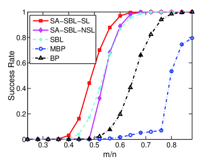
Figure 2: Success rates of respective algorithms vs. the ratio $m/n$.

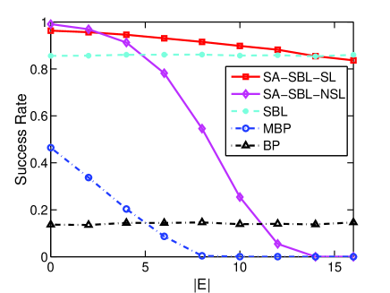
Figure 3: Success rates of respective algorithms vs. the size of the error subset.

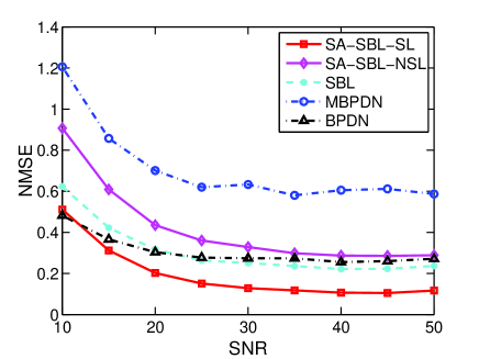
Figure 4: Normalized mean-squared errors of respective algorithms vs. the signal-to-noise ratio.

IV-A Synthetic Data

Suppose a $K$-sparse signal is randomly generated with the support set of the sparse signal randomly chosen according to a uniform distribution. The signals on the support set are independent and identically distributed (i.i.d.) Gaussian random variables with zero mean and unit variance. The measurement matrix $\boldsymbol{A}\in\mathbb{R}^{m\times n}$ is randomly generated with each entry independently drawn from Gaussian distribution with zero mean and unit variance. The prior support information $P$ consists of two subsets: $P=S\cup E$, where $S\subset T$ denotes the subset containing the correct information, and $E\subset T^{c}$ is a subset comprised of false information. In our simulations, only the prior knowledge $P$ is available, the exact partition of $P$ into $S$ and $E$ is unknown. We compare our proposed algorithms with the conventional sparse Bayesian learning (SBL), the basis pursuit (BP) method, and the modified basis pursuit (MBP) method [6] which incorporates the partial support information by assigning different $\ell_{1}$-minimization weights to different coefficients.

We first consider the noiseless case. Fig. 2 plots the success rates of respective algorithms vs. the ratio $m/n$, where we set $K=16$, $n=50$, $|S|=12$ and $|E|=8$, $|S|$ and $|E|$ denote the cardinality (size) of the set $S$ and $E$, respectively. The success rate is computed as the ratio of the number of successful trials to the total number of independent runs. A trial is considered successful if the normalized recovery error, i.e. $\|\boldsymbol{x}-\boldsymbol{\hat{x}}\|_{2}^{2}/\|\boldsymbol{x}\|_{2}^{2}$, is no greater than $10^{-6}$, where $\boldsymbol{\hat{x}}$ denotes the estimate of the true signal $\boldsymbol{x}$. Results are averaged over 1000 independent runs, with the measurement matrix and the sparse signal randomly generated for each run. It can be seen that our proposed SA-SBL-SL method presents a substantial performance advantage over the SA-SBL-NSL and the SBL methods. The performance gain is primarily due to the fact that the SA-SBL-SL method is able to learn the true support from the partly erroneous knowledge and thus make more effective use of the prior support information. We also observe that when a considerable number of errors are present in the prior knowledge, the methods SA-SBL-NSL and MBP present no advantage over their respective counterparts SBL and BP. To examine the behavior of the SA-SBL-SL method more thoroughly, we fix the number of elements in the set $S$ and increase the number of elements in the error set $E$. Fig. 3 depicts the success rates vs. the number of elements in the error set $E$, where we set $m=25$, $K=16$, $|S|=12$ and $|E|$ varies from $1$ to $15$. As can be seen from Fig. 3, when a fairly accurate knowledge is available, i.e. the number of errors is negligible or small, the SA-SBL-NSL achieves the best performance. This is an expected result since little learning is required at this point. Nevertheless, as the number of elements, $|E|$, increases, the SA-SBL-NSL suffers from substantial performance degradation. As compared with the SA-SBL-NSL, the SA-SBL-SL method provides stable recovery performance through learning the values of $\{b_{i}\}$, and outperforms all other algorithms when prior knowledge contains a considerable number of errors. We, however, notice that the proposed SA-SBL-SL method is surpassed by the conventional SBL method when inaccurate information becomes dominant (e.g. $|E|=15$), in which case even learning brings limited benefits and simply ignoring the error-corrupted prior knowledge seems the best strategy.

We now consider the noisy case where the measurements are contaminated by additive noise. The observation noise is assumed multivariate Gaussian with zero mean and covariance matrix $\sigma^{2}\boldsymbol{I}$. The normalized mean-squared errors (NMSEs) of respective algorithms as a function of signal-to-noise ratio (SNR) are plotted in Fig. 4, where we set $m=25$, $n=50$, $K=16$, $|S|=12$, and $|E|=6$. The NMSE is calculated by averaging normalized squared errors over $10^{3}$ independent runs. The SNR is defined as $\text{SNR(dB)}\triangleq 20\log_{10}(\|\boldsymbol{Ax}\|_{2}/\|\boldsymbol{w}\|_{2})$. The MBP-DN is a noisy version of the MBP method [10]. We observe that the conventional SBL and BP-DN methods outperform their respective counterparts: SA-SBL-NSL and MBP-DN. This, again, demonstrates that SA-SBL-NSL and MBP-DN methods are sensitive to prior knowledge inaccuracies. On the other hand, the proposed SA-SBL-SL method which takes advantage of the support learning presents superiority over both the conventional SBL as well as the SA-SBL-NSL method.

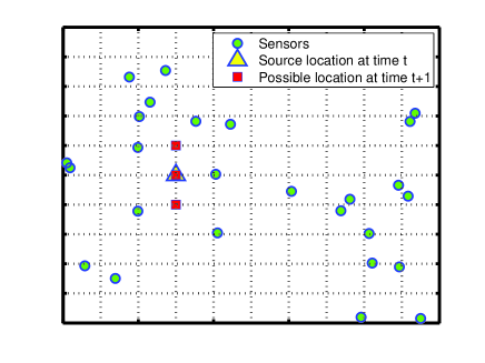
Figure 5: A schematic diagram for source localization.

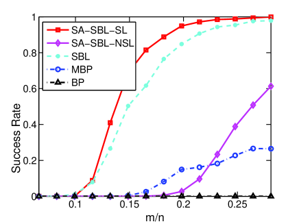
Figure 6: Success rates of respective algorithms vs. the ratio $m/n$ for the noiseless case.

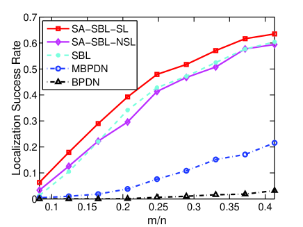
Figure 7: Localization success rates of respective algorithms vs. the ratio $m/n$, $\text{SNR}=20\text{dB}$.

IV-B Source Localization

We consider the problem of intensity-based source localization in sensor networks. The sensing field is partitioned into two-dimensional $n=121$-point virtual grid (Fig. 5) which is used to represent possible locations of the $K=4$ sources. We have $m$ randomly distributed sensors. The measurement collected at sensors can be written as

$$\boldsymbol{y}(t)=\boldsymbol{A}\boldsymbol{x}(t)+\boldsymbol{w}(t)$$

where $\boldsymbol{x}(t)\triangleq[x_{1}(t)\phantom{0}\ldots\phantom{0}x_{n}(t)]^{T}$ is a sparse vector whose entry $x_{i}(t)$ denotes the intensity associated with the $i$th grid point, $\boldsymbol{A}\triangleq[\boldsymbol{a}_{1}\phantom{0}\ldots\phantom{0}\boldsymbol{a}_{m}]^{T}$, $\boldsymbol{a}_{i}^{T}\triangleq[d_{1i}^{-\alpha}\phantom{0}d_{2i}^{-\alpha}\phantom{0}\cdots\phantom{0}d_{ni}^{-\alpha}]$, $d_{ij}$ denotes the distance between the grid point $i$ and the sensor $j$, and $\alpha=2$ is the energy-decay factor.

In practice, sources may keep moving but the current locations’ estimate could still be useful for the future localization. For example, we can expect that some sources may move to grid points close to their previous locations given that the interval between two time instants is sufficiently small. In our simulations, we assume that $K_{1}=3$ sources move slowly such that their next locations are partially predictable based on their current locations. Specifically, for these $K_{1}$ sources, each source either stays at its current position or moves to two of its immediate neighboring grid points at the next time point (see Fig. 5). For simplicity, suppose $\hat{S}=\{\hat{s}_{1},\ldots,\hat{s}_{K_{1}}\}$ is the set of locations associated with the $K_{1}$ sources at time instant $t$, then the set of possible locations of these $K_{1}$ sources at time instant $t+1$ is given by $P=\{\hat{s}_{1}-1,\hat{s}_{1},\hat{s}_{1}+1,\ldots,\hat{s}_{K_{1}}-1,\hat{s}_{K_{1}},\hat{s}_{K_{1}}+1\}$. The set $P$ can serve as prior support knowledge for source localization at time instant $t+1$. Nevertheless, the knowledge $P$ is partly erroneous since all possible locations of these $K_{1}$ sources in the next move are included. For the rest $K-K_{1}$ sources, their locations are randomly chosen from the rest $n-|P|$ grid points. To test the effectiveness of respective algorithms in utilizing the prior knowledge, we assume the locations of these $K_{1}$ sources at time instant $t$ are perfectly known to us and examine the recovery performance at time instant $t+1$. Fig. 6 depicts the success rates vs. the ratio $m/n$ for the noiseless case. Results are averaged over 1000 independent runs, with sensors and locations of sources at time instant $t$ randomly generated for each run. From Fig. 6, we see that the SA-SBL-NSL method yields performance much worse than the conventional SBL method. This is not surprising since the prior knowledge contains a substantial amount of erroneous information. It is also observed that the proposed SA-SBL-SL method which has the ability to learn the true support from erroneous information achieves a significant performance improvement over the SA-SBL-NSL method. We now consider a noisy case where the measurements are corrupted by additive Gaussian noise. When noise is present, exact recovery of sparse signals is impossible. Nevertheless, accurate localization can still be achieved since reliable recovery of the support of sparse signals in the presence of noise is possible. In our simulations, locations of sources are estimated as the grid points associated with the largest $K$ nonzero coefficients of the estimated signal. Fig. 7 plots the localization success rates as a function of the ratio $m/n$, where the signal-to-noise ratio (SNR) is set to $20\text{dB}$. The localization success rate is calculated as the the ratio of the number of successful trials to the total number of independent runs. A trial is considered successful if all $K$ sources’ locations are estimated correctly. Fig. 7, again, demonstrates the superiority of the proposed SA-SBL-SL method over the SA-SBL-NSL and the conventional SBL methods.

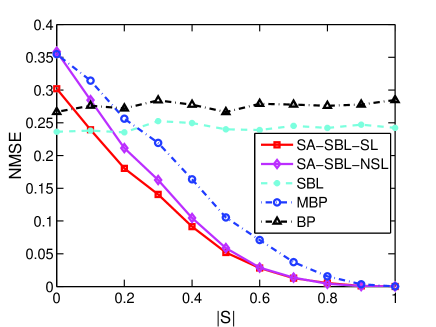
Figure 8: Normalized mean squared errors of respective algorithms vs. the cardinality of the subset $|S|$.

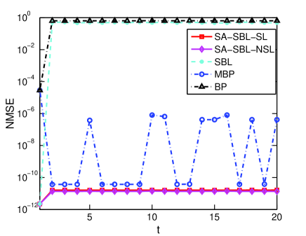
Figure 9: Reconstruction of the sparsified $32\times 32$ larynx sequence. Normalized mean squared errors vs. $t$.

IV-C MRI Data

In this subsection, we carry out experiments on MRI images and sequences. Images have sparse (or approximately sparse) structures in discrete wavelet transform (DWT) basis. By representing an image as a one-dimensional vector, the two-dimensional DWT (a two-level Daubechies-4 wavelet is used) of an image can be expressed as a product of an orthonormal matrix $\boldsymbol{\Psi}$ and the image vector $\boldsymbol{x}$. The sensing matrix $\boldsymbol{A}$ is therefore equal to $\boldsymbol{A}=\boldsymbol{Q}\boldsymbol{\Psi}$, where $\boldsymbol{Q}$ denotes the measurement acquisition matrix and its entries are i.i.d. normal random variables. We test all algorithms on sparsified images. Similar to [6], the image is sparsified by computing its 2D-DWT, retaining the coefficients from the $99\%$-energy support while setting others to zero and taking the inverse DWT.

We first evaluate the reconstruction performance of respective algorithms for a sparsified image. The image is a $32\times 32$ larynx image obtained by resizing the $256\times 256$ larynx image, i.e. $n=1024$. For this image, its support size is $|T|=70$. In our experiments, we fix the size of the set $E$ to be $|E|=0.4|T|$, and gradually increase the size of the set $S$. Fig. 8 depicts the NMSEs of respective algorithms vs. the size of $S$, where $m=0.55n$ and $|S|$ varies from $0$ to $0.9|T|$. Results are averaged over 500 independent runs, with the acquisition matrix $\boldsymbol{Q}$, the sets $E$ and $S$ randomly generated for each run. From Fig. 8, we see that when the prior support knowledge is dominated by the error set $E$, the SBL and BP methods outperform their respective “support-aided” counterparts SA-SBL-NSL and MBP. Nevertheless, the SA-SBL-NSL and the MBP methods surpass and eventually achieve a significant performance improvement over the SBL and BP methods as the prior knowledge becomes more and more accurate. It can also be observed the SA-SBL-SL method presents uniform superiority over SA-SBL-NSL and MBP for different values of $|S|$, and the performance gap is wider in the small $|S|$’s region since learning in this region apparently brings more significant benefits as compared with learning in the large $|S|$’s region.

We also conduct a comparison for the sparsified $32\times 32$ larynx sequence in Fig. 9. Since the support of the sequence undergoes a small variation, the prior support knowledge can be obtained as the estimate of the previous time instant. At the very beginning, i.e. $t=0$, the prior knowledge set $P$ is empty. Conventional SBL and BP methods are then used to obtain an initial support estimate for their respective support-aided methods. We set $m_{0}=0.6n$ in order to ensure a fairly accurate initial estimate is obtained. For $t>0$, only $m_{t}=0.3n$ measurements are collected for the signal reconstruction. From Fig. 9, we see that the all support-aided methods including SA-SBL-SL, SA-SBL-NSL and MBP are able to achieve exact reconstruction with only as few as $m=0.3n$ measurements, whereas the conventional SBL and BP fail to recover the signal with these few measurements. Also, since the prior support knowledge is fairly accurate, support learning does not bring any additional benefits, and thus both the SA-SBL-SL and SA-SBL-NSL methods attain similar recovery performance.

V Conclusions

We studied the problem of sparse signal recovery given that part of the signal’s support is known a priori. The prior knowledge, however, may not be accurate and could contain erroneous information. This knowledge inaccuracy may result considerable performance degradation or even recovery failure. To address this issue, we first introduced a modified two-layer Gaussian-inverse Gamma hierarchical prior model. The modified two-layer model employs an individual parameter $b_{i}$ for each sparsity-controlling hyperparameter $\alpha_{i}$, and therefore has the ability to place non-sparsity-encouraging priors to those coefficients that are believed in the support set. Based on this two-layer mode, we then proposed an improved three-layer hierarchical prior model, with a prior placed on the parameters $\{b_{i}\}$ in the third layer. Such a model enables to automatically learn the true support from partly erroneous information through learning the values of $\{b_{i}\}$. Bayesian algorithms are developed by resorting to the mean field variational Bayes. Simulation results show that substantial performance improvement can be achieved through support learning since it allows us to make more effective use of the partly erroneous information.

References

- [1] S. S. Chen, D. L. Donoho, and M. A. Saunders, “Atomic decomposition by basis pursuit,” SIAM J. Sci. Comput., vol. 20, no. 1, pp. 33–61, 1998.
- [2] E. Candés and T. Tao, “Decoding by linear programming,” IEEE Trans. Information Theory, no. 12, pp. 4203–4215, Dec. 2005.
- [3] D. L. Donoho, “Compressive sensing,” IEEE Trans. Inform. Theory, vol. 52, pp. 1289–1306, 2006.
- [4] J. A. Tropp and A. C. Gilbert, “Signal recovery from random measurements via orthogonal matching pursuit,” IEEE Trans. Information Theory, vol. 53, no. 12, pp. 4655–4666, Dec. 2007.
- [5] M. J. Wainwright, “Information-theoretic limits on sparsity recovery in the high-dimensional and noisy setting,” IEEE Trans. Information Theory, vol. 55, no. 12, pp. 5728–5741, Dec. 2009.
- [6] N. Vaswani and W. Lu, “Modified-CS: modifying compressive sensing for problems with partially known support,” IEEE Trans. Signal Processing, no. 9, pp. 4595–4607, September 2010.
- [7] N. Vaswani, “LS-CS-residual (LS-CS): compressive sensing on least squares residual,” IEEE Trans. Signal Processing, no. 8, pp. 4108–4120, August 2010.
- [8] M. A. Khajehnejad, W. Xu, A. S. Avestimehr, and B. Hassibi, “Weighted minimization for sparse recovery with prior information,” in Proc. IEEE Int. Symp. Information Theory, Seoul, Korea, June 28–July 3 2009.
- [9] C. J. Miosso, R. von Borries, M. Argaez, L. Velazquez, C. Quintero, and C. M. Potes, “Compressive sensing reconstruction with prior information by iteratively reweighted least-squares,” IEEE Trans. Signal Processing, no. 6, pp. 2424–2431, June 2009.
- [10] W. Lu and N. Vaswani, “Regularized modified BPDN for noisy sparse reconstruction with partial erroneous support and signal value knowledge,” IEEE Trans. Signal Processing, no. 1, pp. 182–196, January 2012.
- [11] J. Ziniel and P. Schniter, “Dynamic compressive sensing of time-varying signals via approximate message passing,” IEEE Trans. Signal Processing, no. 21, pp. 5270–5284, Nov. 2013.
- [12] J. Fang, Y. Shen, and H. Li, “Pattern coupled sparse bayesian learning for recovery of time-varying sparse signals,” in 19th International Conference on Digital Signal Processing, Hong Kong, August 20–23 2014.
- [13] M. Tipping, “Sparse Bayesian learning and the relevance vector machine,” Journal of Machine Learning Research, vol. 1, pp. 211–244, 2001.
- [14] D. P. Wipf, “Bayesian methods for finding sparse representations,” Ph.D. dissertation, University of California, San Diego, 2006.
- [15] S. Ji, Y. Xue, and L. Carin, “Bayesian compressive sensing,” IEEE Trans. Signal Processing, vol. 56, no. 6, pp. 2346–2356, June 2008.
- [16] D. P. Wipf and B. D. Rao, “An empirical Bayesian strategy for solving the simultaneous sparse approximation problem,” IEEE Trans. Signal Processing, vol. 55, no. 7, pp. 3704–3716, July 2007.
- [17] Z. Zhang and B. D. Rao, “Sparse signal recovery with temporally correlated source vectors using sparse Bayesian learning,” IEEE Journal of Selected Topics in Signal Processing, vol. 5, no. 5, pp. 912–926, Sept. 2011.
- [18] D. G. Tzikas, A. C. Likas, and N. P. Galatsanos, “The variational approximation for Bayesian inference,” IEEE Signal Processing Magazine, pp. 131–146, Nov. 2008.