Analytical solutions of a fractional diffusion-advection equation for solar cosmic-ray transport

Abstract

Motivated by recent applications of superdiffusive transport models to shock-accelerated particle distributions in the heliosphere, we solve analytically a one-dimensional fractional diffusion-advection equation for the particle density. We derive an exact Fourier transform solution, simplify it in a weak diffusion approximation, and compare the new solution with previously available analytical results and with a semi-numerical solution based on a Fourier series expansion. We apply the results to the problem of describing the transport of energetic particles, accelerated at a traveling heliospheric shock. Our analysis shows that significant errors may result from assuming an infinite initial distance between the shock and the observer. We argue that the shock travel time should be a parameter of a realistic superdiffusive transport model.

1. Introduction

When energetic particles, accelerated in the solar corona or the solar wind, propagate in a turbulent heliospheric medium, the particle transport is often diffusive (Parker, 1965). The diffusion approximation is a standard tool in the description of evolving cosmic-ray distributions (e.g. Schlickeiser & Shalchi, 2008; Artmann et al., 2011, and references therein).

A generalization of the diffusion equation is obtained by replacing the usual derivatives by fractional derivatives. Formally, standard diffusion, characterized by a linear growth of the variance of a particle displacement, separates the processes of faster superdiffusion and slower subdiffusion (e.g., Saichev & Zaslavsky, 1997). These processes are governed by partial differential equations with fractional operators (Samko et al., 1993). Physically, fractional differential equations conveniently describe stochastic transport when an effective mean free path is comparable with a macroscopic length scale. The corresponding diffusive process is non-local: it is described by an integral equation that can be rewritten in terms of fractional derivatives (for a clear discussion, see Chukbar, 1995).

In sharp contrast to classical diffusion, solutions to fractional diffusion equations typically are not Gaussian but rather have power-law tails. The key question in concrete applications is whether the approach only provides a phenomenological parametrization for the data or the postulated anomalous diffusion is based on physical processes that can be described by a fractional evolution equation (see, e.g., Metzler & Klafter, 2000; Perrone et al., 2013, for numerous potential applications).

Observed solar cosmic-ray particle distributions often appear to exhibit power-law tails, suggesting an interpretation in terms of superdiffusion. Distributions of electrons and protons, accelerated both in the solar corona and at interplanetary shocks, have recently been analyzed in terms of superdiffusive transport models (Perri & Zimbardo, 2007, 2009; Sugiyama & Shiota, 2011; Trotta & Zimbardo, 2011; Zimbardo & Perri, 2013). Notably, those studies relied on an asymptotic expression for a non-Gaussian propagator (equivalent to the Green’s function of a fractional diffusion equation), which has a limited validity range.

In this paper we develop more accurate analytical solutions and argue that they should be used to put the superdiffusive particle transport in the heliosphere on a firmer footing. As a concrete example, we examine a prototypical transport problem, described by a one-dimensional fractional diffusion-advection equation (Section 2). We derive an exact solution by the Fourier transform (Section 3), and we obtain an approximate solution in terms of elementary functions in a weak diffusion approximation (Section 4). We demonstrate the accuracy of the approximation by comparing the new solution with a semi-numerical solution based on a formally exact Fourier series expansion (Section 5), and we discuss what our results imply for the interpretation of the observed particle distributions as evidence of superdiffusive transport in the heliosphere (Section 6).

2. Formulation of the problem

Consider first the usual diffusion-advection equation for a one-dimensional particle distribution function $f(x,t)$ that depends on position $x$ and time $t>0$:

$$\frac{\partial f}{\partial t}=\kappa\frac{\partial^{2}f}{\partial x^{2}}+a\frac{\partial f}{\partial x}+\delta(x).$$ (1)

Here $a$ is a constant advection speed, and $\kappa$ is a constant diffusion coefficient. This transport equation follows from the Fokker–Planck equation for energetic particles if their energy losses are neglected and pitch-angle scattering is strong (e.g., Schlickeiser & Shalchi, 2008; Litvinenko & Schlickeiser, 2013, and references therein). A delta-functional source term on the right may correspond to energetic particles injected at a shock, and $a$ can be interpreted as the background solar wind speed.

Standard methods (e.g., Carslaw & Jaeger, 1959) give the solution of the initial value problem $f(x,0)=0$ on the interval $-\infty<x<\infty$:

$$f(x,t)=\int_{0}^{t}(4\pi\kappa t^{\prime})^{-1/2}\exp\left[-\frac{(x+at^{\prime})^{2}}{4\kappa t^{\prime}}\right]dt^{\prime}.$$ (2)

A steady distribution is established in the limit $t\to\infty$:

$$f(x,\infty)=\frac{1}{a}\exp\left(-\frac{a}{\kappa}x\right),\quad x>0,$$ (3)

$$f(x,\infty)=a^{-1},\quad x<0.$$ (4)

In the remainder of the paper, we investigate the following fractional differential equation that generalizes the usual diffusion-advection equation:

$$\frac{\partial f}{\partial t}=\kappa\frac{\partial^{\alpha}f}{\partial|x|^{\alpha}}+a\frac{\partial f}{\partial x}+\delta(x)$$ (5)

(e.g., Stern et al., 2014). The equation governs the evolution of a distribution function $f(x,t)$ for $t>0$ and $-\infty<x<\infty$. For simplicity, we assume the initial condition

$$f(x,0)=0.$$ (6)

The advection speed $a$ and diffusion coefficient $\kappa$ (now with dimensions length^α/time) are positive constants. We use the Riesz derivative to define a fractional spatial derivative:

$$\frac{\partial^{\alpha}f(x,t)}{\partial|x|^{\alpha}} =\frac{1}{\pi}\sin\left(\frac{\pi}{2}\alpha\right)\Gamma(1+\alpha)$$

$$\times\int_{0}^{\infty}\frac{f(x+\xi)-2f(x)+f(x-\xi)}{\xi^{1+\alpha}}d\xi$$ (7)

(Samko et al., 1993; Saichev & Zaslavsky, 1997). Because the derivative corresponds to a fractional Laplacian operator in higher dimensions, an alternative notation $-(-\Delta)^{\alpha/2}f$ is also used (Mainardi et al., 2001). Although the regularized form above is defined for $0<\alpha<2$, in what follows we are mainly interested in the superdiffusive case $1<\alpha<2$.

3. Fourier transform solution and asymptotics

The Fourier transform gives a convenient method of solving the fractional diffusion-advection equation on the interval $-\infty<x<\infty$. Taking the Fourier transform of equation (5) yields

$$\frac{\partial\tilde{f}}{\partial t}=-\kappa|k|^{\alpha}\tilde{f}+iak\tilde{f}+\frac{1}{2\pi},$$ (8)

where

$$\tilde{f}(k,t)=\frac{1}{2\pi}\int_{-\infty}^{\infty}f(x,t)\exp(-ikx)dx.$$ (9)

Integration of the first-order equation for $\tilde{f}$ yields

$$\tilde{f}(k,t)=\frac{1}{2\pi}\frac{1-\exp[(iak-\kappa|k|^{\alpha})t]}{\kappa|k|^{\alpha}-iak},$$ (10)

where an integration constant is specified by the initial condition $\tilde{f}(k,0)=0$. Now the inverse Fourier transform gives the solution

$$f(x,t)=\frac{1}{2\pi}\int_{-\infty}^{\infty}\frac{1-\exp[(iak-\kappa|k|^{\alpha})t]}{\kappa|k|^{\alpha}-iak}\exp(ikx)dk.$$ (11)

In the non-diffusive case, $\kappa=0$ and the integral is evaluated to give an expanding “top-hat” solution

$$\left.f(x,t)\right|_{\kappa=0}=f_{0}(x,t)=\frac{1}{2a}\left[\mbox{sgn}(x+at)-\mbox{sgn}(x)\right].$$ (12)

The solution of equation (5) can also be expressed as

$$f(x,t)=\int_{0}^{t}G(x+at^{\prime},t^{\prime})dt^{\prime},$$ (13)

where the Green’s function $G(x,t)$ satisfies the fractional diffusion equation

$$\frac{\partial G}{\partial t}=\kappa\frac{\partial^{\alpha}G}{\partial|x|^{\alpha}}+\delta(x)\delta(t).$$ (14)

Its Fourier transform is given by

$$\frac{\partial\tilde{G}}{\partial t}=-\kappa|k|^{\alpha}\tilde{G}+\frac{1}{2\pi}\delta(t).$$ (15)

It follows that

$$\tilde{G}(k,t)=\frac{1}{2\pi}\exp(-\kappa|k|^{\alpha}t),$$ (16)

and the inverse Fourier transform yields

$$G(x,t)=\frac{1}{\pi}\int_{0}^{\infty}\exp(-\kappa k^{\alpha}t)\cos(kx)dk$$ (17)

(e.g., Chukbar, 1995).

An asymptotic expression for $G(x,t)$ is obtained by integrating equation (17) by parts and applying an analogue of Watson’s lemma for Fourier type integrals (e.g., Ablowitz & Fokas, 1997). For $x\gg(\kappa t)^{1/\alpha}$, the result is

$$G(x,t)\approx\frac{1}{\pi}\sin\left(\frac{\pi}{2}\alpha\right)\Gamma(1+\alpha)\frac{\kappa t}{|x|^{1+\alpha}}.$$ (18)

For $x>0$, substitution into equation (13) yields

$$f(x,t)\approx\frac{1}{\pi}\sin\left(\frac{\pi}{2}\alpha\right)\Gamma(1+\alpha)\int_{0}^{t}\frac{\kappa t^{\prime}}{(x+at^{\prime})^{1+\alpha}}dt^{\prime},$$ (19)

and so the distribution function $f(x,t)$ is given by

$$f(x,t)\approx\frac{1}{\pi}\sin\left(\frac{\pi}{2}\alpha\right)\Gamma(\alpha-1)\frac{\kappa}{a^{2}}\left[x^{1-\alpha}-\frac{x+\alpha at}{(x+at)^{\alpha}}\right]$$ (20)

as long as $x+at\gg(\kappa t)^{1/\alpha}$ and $1<\alpha<2$. Two limiting cases are as follows:

$$f(x,t) \approx\frac{1}{2\pi}\sin\left(\frac{\pi}{2}\alpha\right)\Gamma(1+\alpha)\frac{\kappa t^{2}}{x^{1+\alpha}},\quad x\gg at,$$ (21)

$$f(x,t) \approx\frac{1}{\pi}\sin\left(\frac{\pi}{2}\alpha\right)\Gamma(\alpha-1)\frac{\kappa}{a^{2}}x^{1-\alpha},\quad 0<x\ll at.$$ (22)

Equation (22) is essentially the asymptotic power-law that was previously used in the data analysis of energetic particles, accelerated in the solar corona (Trotta & Zimbardo, 2011) and at interplanetary shocks (Perri & Zimbardo, 2007, 2009; Sugiyama & Shiota, 2011). For instance, Perri & Zimbardo (2007, 2009) used a formula for the particle density at a fixed point due to a shock-associated source moving with a speed $V_{\rm sh}$. The formula follows from our analysis by changing the reference frame. Suppose a shock, initially located at $x_{0}=-V_{\rm sh}t_{0}$, moves at speed $V_{\rm sh}$ and arrives at $x=0$ when $t=0$. On changing variables, equation (20) yields

$$f(x,t) \approx\frac{1}{\pi}\sin\left(\frac{\pi}{2}\alpha\right)\Gamma(\alpha-1)\frac{\kappa}{V_{\rm sh}^{2}}$$ (23)

$$\times\left[(x-V_{\rm sh}t)^{1-\alpha}-\frac{x+(\alpha-1)V_{\rm sh}t+\alpha V_{\rm sh}t_{0}}{(x+V_{\rm sh}t_{0})^{\alpha}}\right]\,,$$

which reduces to equation (4) in Perri & Zimbardo (2007) on assuming that the shock is coming from a very large distance, $t_{0}\to\infty$. Note for clarity that Perri & Zimbardo (2007) do not specify a normalization constant $b$ in their equation (1), and their notation is different: their $\mu$ is our $1+\alpha$, and their $\alpha$ is our $3-\alpha$. The latter expression appears in the dependence of the variance of a particle displacement on time $\sim t^{3-\alpha}$ when a finite particle speed is taken into account.

4. A weak diffusion approximation

A limitation of the analysis in the previous section is that we used a short-time asymptotic (18) for the Green’s function $G(x,t)$ to derive equation (20) for the particle distribution function $f(x,t)$, and so it is not clear whether the results are valid for $at\gg x$. In addition, the results are only valid for $x>0$ because the integral in equation (13) diverges for $x<0$ if equation (18) is used to evaluate the integral. To remove these limitations of the analysis, we solve for $f(x,t)$ in a weak diffusion approximation that allows us to evaluate the integral in equation (11) for both $x>0$ and $x<0$.

The superdiffusive term in equation (5) can be treated as a perturbation sufficiently far from the locations where the advective solution (12) predicts jumps in $f(x,t)$. Suppose $l_{d}$ is the distance from a jump where the diffusive and advective terms in equation (5) are comparable. To an order of magnitude, $\kappa\partial^{\alpha}f/\partial|x|^{\alpha}\sim\kappa f/l_{d}^{\alpha}$ and $a\partial f/\partial x\sim af/l_{d}$. The diffusion length is thus defined as

$$l_{d}=(\kappa/a)^{1/(\alpha-1)}.$$ (24)

Now assuming that

$$l_{d}\ll|x|,|x+at|,at,$$ (25)

we can formally treat $\kappa$ as a small parameter, and so

$$f(x,t)\approx f_{0}(x,t)+\kappa\left.\frac{df(x,t)}{d\kappa}\right|_{\kappa=0},$$ (26)

where $f_{0}(x,t)$ is given by equation (12). Differentiation of equation (11) with respect to $\kappa$ yields

$$f(x,t) \approx f_{0}(x,t)$$

$$+\frac{\kappa}{\pi a^{2}}\int_{0}^{\infty}\biggl{[}\frac{\cos kx-\cos k(x+at)}{k^{2-\alpha}}$$

$$-\frac{(\alpha-1)at}{(x+at)}\frac{\cos k(x+at)}{k^{2-\alpha}}\biggr{]}dk,$$ (27)

where the last term in the integrand is obtained by integrating by parts and neglecting a rapidly varying term containing $\exp[ik(x+at)]$ at the upper integration limit. On simplifying and using Watson’s lemma, we get

$$f(x,t) \approx f_{0}(x,t)+\frac{1}{\pi}\sin\left(\frac{\pi}{2}\alpha\right)\Gamma(\alpha-1)\frac{\kappa}{a^{2}}$$

$$\times\left[|x|^{1-\alpha}-\frac{x+\alpha at}{(x+at)|x+at|^{\alpha-1}}\right].$$ (28)

For $x>0$, we recover equation (20) and its limiting cases, confirming the analysis of the previous section. For $x<0$, we have

$$f(x,t)\approx\frac{1}{2\pi}\sin\left(\frac{\pi}{2}\alpha\right)\Gamma(1+\alpha)\frac{\kappa t^{2}}{|x|^{1+\alpha}},\quad|x|\gg at,$$ (29)

$$f(x,t)\approx\frac{1}{a}+\frac{1}{\pi}\sin\left(\frac{\pi}{2}\alpha\right)\Gamma(\alpha-1)\frac{\kappa}{a^{2}}|x|^{1-\alpha},\quad|x|\ll at.$$ (30)

The discontinuity at $x=-at$ broadens into a smoother transition. The solution is inapplicable in the vicinity of the jump at $|x+at|\approx 0$, however, because the weak diffusion approximation is valid only as long as $|x|$, $|x+at|$, and $at$ are large in comparison with the diffusion length $l_{d}$,

5. Accuracy of the approximation

Stern et al. (2014) gave the following exact Fourier series solution to equation (5) on a domain of length $L$:

$$f(x,t) =\sum_{n=1}^{\infty}\Biggl{\{}(1+(-1)^{n+1})\biggl{[}\left(\frac{n\pi}{L}\right)^{\alpha}\kappa L\cos\left(\frac{n\pi x}{L}\right)$$

$$-n\pi a\sin\left(\frac{n\pi}{L}x\right)$$

$$-\left(\frac{n\pi}{L}\right)^{\alpha}\kappa L\cos\left(\frac{n\pi}{L}(x+at)\right)\exp\left(-\left(\frac{n\pi}{L}\right)^{\alpha}\kappa t\right)$$

$$+n\pi a\sin\left(\frac{n\pi}{L}(x+at)\right)\exp\left(-\left(\frac{n\pi}{L}\right)^{\alpha}\kappa t\right)\biggr{]}\text{\Huge{/}}$$

$$\left(\left(\frac{n\pi}{L}\right)^{2\alpha}\kappa^{2}L^{2}+n^{2}\pi^{2}a^{2}\right)\Biggr{\}}\,.$$ (31)

Because $f(x,t)=f(x+2L,t)$, the series does not represent the solution of an initial-value problem on an infinite interval for $t\rightarrow\infty$. For a localized source and finite $t$, however, the series solution accurately represents $f(x,t)$ on an infinite interval if $L$ is sufficiently large. In practice, we achieve accuracy by choosing $L\gg at$.

We compare the new analytical solutions of the previous sections with a semi-numerical solution based on the Fourier series expansion. We use equation (5) and sum up $N=10^{6}$ terms with $L=1000$ to achieve high accuracy. We set $a=1$, which simply means that in what follows we measure speeds in units of the solar wind speed. We choose $\alpha=1.5$ in agreement with the range of values inferred from the heliospheric particle data (Perri & Zimbardo, 2007, 2009; Sugiyama & Shiota, 2011). The superdiffusion coefficient $\kappa$ is a key parameter of the theory. Work is underway to estimate $\kappa$ from the data (Perri et al., in preparation). We adopt $\kappa=0.5$ as an illustration and investigate how the particle distribution evolves over a few hundred advection times.

Figure 1 shows the results in a semi-logarithmic plot at time $t=10$. We find a good agreement between the analytical (solid black line) and semi-numerical (black symbols) solutions, except for the region around $x=-at$ where the weak diffusion approximation is not valid. The red box in the figure illustrates the non-diffusive solution given by equation (12). We have truncated the analytical solution in the vicinity of $x=-at$ over a length $l$ of ten times the diffusion length ($l=10\,l_{d}=2.5$). The green and blue lines give the steady-state solution for the Gaussian diffusion case, given by equation (3), and the approximate steady-state solution, given by equation (30).

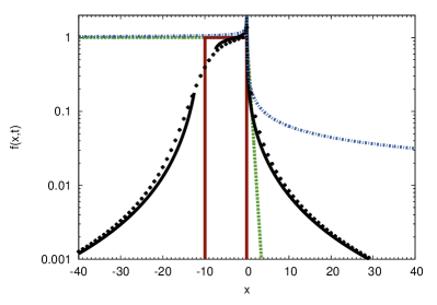
Figure 1.— The Fourier transform solution in a weak diffusion limit (equation (28), solid black line) and the series solution (equation (5), black symbols) at time $t=10$. The dot-dashed blue line gives the approximate steady solution in equation (22) for $x>0$ and equation (30) for $x<0$. For reference, the dashed green line shows the steady state Gaussian diffusion solution in equation (3), and the red box shows the expanding top-hat non-diffusive solution in equation (12). Parameters are $\alpha=1.5$, $\kappa=0.5$, $a=1$.

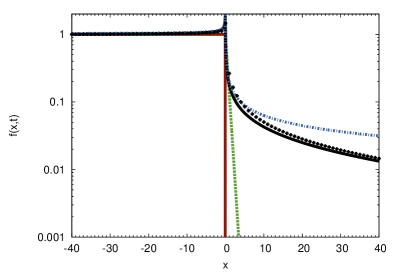
Figure 2.— Same as Figure 1 but now at time $t=200$.

Figure 2 gives the same solutions as in Figure 1 at a later time $t=200$. The weak diffusion solution and the Fourier series remain in good agreement as they slowly approach the steady state. The downstream region in Figure 2 is already completely filled since $|x|\ll at$. An interesting feature of the solution is a peak at the injection site $x=0$, which is not present for Gaussian diffusion.

6. Discussion

We used the Fourier transform to solve analytically a fractional diffusion-advection equation for cosmic ray transport, and we applied the solution to the problem of describing the transport of energetic particles, accelerated at a traveling heliospheric shock. We also developed a weak diffusion approximation, based on the exact Fourier transform solution. We confirmed the validity of the approximation for both early and late times by comparing it with an exact Fourier series solution. Our analysis is motivated by recent applications of superdiffusive transport models to the observed shock-accelerated particle distributions (Perri & Zimbardo, 2007, 2009; Sugiyama & Shiota, 2011).

Our new solution quantifies the limited validity of the asymptotic expressions, used previously to interpret the particle data. Specifically, the formula used by Perri & Zimbardo (2007, 2009) and Sugiyama & Shiota (2011) is basically our equation (23) in the limit $t_{0}\to\infty$, corresponding to a shock approaching an observer from a very large distance $V_{\rm sh}t_{0}$. As our results show, however, it may take a very long time for the asymptotic expression to become accurate. The ratio of the second term in equation (23) to the first one is $(-t/t_{0})^{\alpha-1}(\alpha+(\alpha-1)t/t_{0})$ at $x=0$, and so our more accurate solution differs from the $t_{0}=\infty$ asymptotic expression by about a factor of 2 when the distance between the observer and the shock is as short as one tenth of the initial distance $V_{\rm sh}t_{0}$ between them.

To sum up, solar cosmic-ray data in various settings appear to be consistent with asymptotic propagator solutions to a fractional diffusion equation or more general continuous-time random-walk models (Zimbardo & Perri, 2013). We argued, however, that more accurate solutions of an appropriate transport equation should be used for validating the superdiffusive transport of energetic particles in the heliosphere. In the context of the transport of particles, accelerated at a traveling heliospheric shock, our analysis strongly suggests that we should not assume the initial distance $V_{\rm sh}t_{0}$ of the shock from the observer to be infinite. The shock travel time $t_{0}$ should be a parameter of the superdiffusive transport model.

References

- Ablowitz & Fokas (1997) Ablowitz, M. J., & Fokas, A. S. 1997, Complex Variables: Introduction and Applications (Cambridge University Press)
- Artmann et al. (2011) Artmann, S., Schlickeiser, R., Agueda, N., Krucker, S., & Lin, R. P. 2011, A&A, 535, A92
- Carslaw & Jaeger (1959) Carslaw, H. S., & Jaeger, J. C. 1959, Conduction of Heat in Solids (Oxford: Clarendon Press)
- Chukbar (1995) Chukbar, K. V. 1995, Soviet Journal of Experimental and Theoretical Physics, 81, 1025
- Litvinenko & Schlickeiser (2013) Litvinenko, Y. E., & Schlickeiser, R. 2013, A&A, 554, A59
- Mainardi et al. (2001) Mainardi, F., Luchko, Y., & Pagnini, G. 2001, Fract. Calc. Appl. Analys., 4, 153
- Metzler & Klafter (2000) Metzler, R., & Klafter, J. 2000, Phys. Rep., 339, 1
- Parker (1965) Parker, E. N. 1965, Planet. Space Sci., 13, 9
- Perri & Zimbardo (2007) Perri, S., & Zimbardo, G. 2007, ApJ, 671, L177
- Perri & Zimbardo (2009) —. 2009, ApJ, 693, L118
- Perrone et al. (2013) Perrone, D., et al. 2013, Space Sci. Rev., 178, 233
- Saichev & Zaslavsky (1997) Saichev, A. I., & Zaslavsky, G. M. 1997, Chaos, 7, 753
- Samko et al. (1993) Samko, S., Kilbas, A., & Marichev, O. 1993, Fractional Integrals and Derivatives: Theory and Applications (Gordon and Breach Science Publishers)
- Schlickeiser & Shalchi (2008) Schlickeiser, R., & Shalchi, A. 2008, ApJ, 686, 292
- Stern et al. (2014) Stern, R., Effenberger, F., Fichtner, H., & Schäfer, T. 2014, Fract. Calc. Appl. Analys., 17, 171
- Sugiyama & Shiota (2011) Sugiyama, T., & Shiota, D. 2011, ApJ, 731, L34
- Trotta & Zimbardo (2011) Trotta, E. M., & Zimbardo, G. 2011, A&A, 530, A130
- Zimbardo & Perri (2013) Zimbardo, G., & Perri, S. 2013, ApJ, 778, 35