Of chain–based order and quantum spin liquids in dipolar spin ice

Abstract

Recent experiments on the spin–ice material Dy₂Ti₂O₇ suggest that the Pauling “ice entropy”, characteristic of its classical Coulombic spin-liquid state, may be lost at low temperatures [D. Pomaranski et al., Nature Phys. 9, 353 (2013)]. However, despite nearly two decades of intensive study, the nature of the equilibrium ground state of spin ice remains uncertain. Here we explore how long-range dipolar interactions $D$, short-range exchange interactions, and quantum fluctuations combine to determine the ground state of dipolar spin ice. We identify a new organisational principle, namely that ordered ground states are selected from a set of “chain states” in which dipolar interactions are exponentially screened. Using both quantum and classical Monte Carlo simulation, we establish phase diagrams as a function of quantum tunneling $g$, and temperature $T$, and find that only a very small $g_{c}\ll D$ is needed to stabilize a quantum spin-liquid ground state. We discuss the implications of these results for Dy₂Ti₂O₇.

I Introduction

The search for materials which realize a spin-liquid state, in which magnetic moments interact strongly, and yet fail to order, has become something of a cause célèbre.fazekas74 ; lee08 ; balents10 A rare three-dimensional example of a spin liquid is provided by the “spin–ice” materials, a family of rare–earth pycrochlore oxides exemplified by Ho₂Ti₂O₇ and Dy₂Ti₂O₇, which exhibit a “Coulombic” phase — a classical spin liquid, exhibiting an emergent $U(1)$ gauge field, whose excitations famously take the form of magnetic monopoles.bramwell01-Science294 ; castelnovo12 The fate of this spin liquid at low temperatures is an important question, touching on the limits of our understanding of phase transitions,powell11 and the tantalising possibility of finding a quantum spin-liquid in three dimensions. Nonetheless, after nearly two decades of intensive study, the nature of the quantum ground state of spin-ice materials remains a mystery.

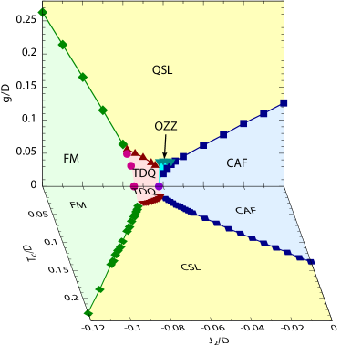
Figure 1: (Color online) Quantum and classical phase diagrams for a spin ice with long-range dipolar interactions $D$, as a function of second-neighbour exchange $J_{2}$. Quantum tunneling $g$, and temperature $T$, drive quantum (QSL) and classical (CSL) spin-liquid phases. These compete with four distinct ordered phases based on ferromagnetically–polarised chains of spins, illustrated in Fig. 2. Results are taken from quantum and classical Monte Carlo simulations of $\mathcal{H_{\sf QDSI}}$ [Eq. (12)], for a cubic cluster of 128 spins, with exchange $J_{k}=0$ for $k\neq 2$.

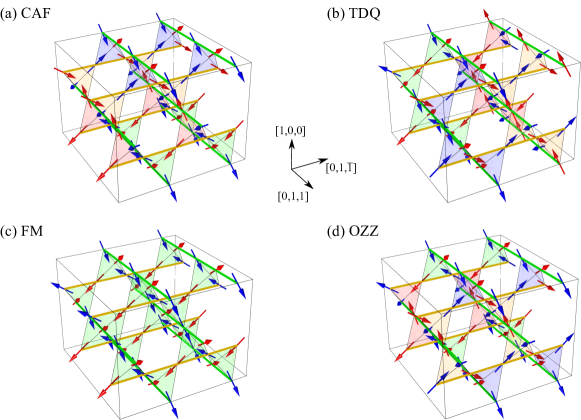
Figure 2: (Color online) Chain–based ordered ground states found in a dipolar spin–ice with competing exchange interactions. (a) cubic antiferromagnet (CAF); (b) tetragonal double-Q state (TDQ); (c) ferromagnet (FM); (d) orthorhombic “zig-zag” (OZZ) state stabilised by quantum fluctuations. All states obey the ice rules, and are composed of chains of spins with net ferromagnetic polarisation (green and yellow lines). Tetrahedra of the same color have the same spin–configuration. Animated images of these ordered states can be found in the supplemental materials.supplemental

This question gains fresh urgency from recent experiments on the spin ice Dy₂Ti₂O₇, pomaranski13 which suggest that the Pauling ice entropy, associated with an extensive number of states obeying the “two-in, two-out” ice rules,ramirez99 ; klemke11 is lost at the lowest temperatures. Such a loss of entropy could herald the onset of a long-range ordered state siddharthan99 ; siddharthan-arXiv ; denHertog00 ; bramwell01-PRL87 ; melko01 , in which magnetic monopoles would be confined. Alternatively, it could signal the emergence of a three-dimensional quantum spin-liquid, in which monopoles would remain deconfined. The theoretical possibility of such a spin-liquid has been widely discussed, hermele04 ; banerjee08 ; savary12 ; shannon12 ; benton12 ; lee12 ; savary13 ; gingras14 ; hao-arXiv ; kato-arXiv and is now well-established through quantum Monte Carlo simulations of models with anisotropic nearest-neighbour exchange. banerjee08 ; shannon12 ; benton12 ; kato-arXiv These results have generated considerable excitement in the context of recent experiments on “quantum spin ice” systems such as Yb₂Ti₂O₇, thompson11 ; ross11-PRX1 ; chang12 , Tb₂Ti₂O₇, molovian07 ; fennell12 ; fennell14 and Pr₂Zr₂O₇. kimura13 However they leave unanswered the question of what happens in a realistic model of a spin ice such as Dy₂Ti₂O₇. Moreover, the long equilibration time–scales encountered in both simulation melko01 and experiment pomaranski13 suggests that it is difficult to access one low–energy spin configuration from another. It is therefore important to understand the nature of the different low–energy spin configurations in a realistic model — could a new organisational principle be in play ?

In this Article we address the question : “What determines the equilibrium ground state of spin ice, once quantum effects are taken into account ?” We start from a realistic model, directly motivated by experiment, which treats both short-range exchange and long-range dipolar interactions, as well as quantum tunneling between different spin–ice configurations. Our main theoretical results are summarized in the combined quantum and classical phase diagram Fig. 1, with illustrations of possible ordered ground states given in Fig. 2.

We first consider the classical ground state of dipolar spin ice, in the absence of quantum fluctuations. We find that long–range dipolar interactions are minimised by spin–configurations composed of chains of spins with net ferromagnetic polarisation. We show that, within these “chain states”, dipolar interactions are exponentially screened and that all potential classical ground states can be described by a mapping onto an effective Ising model on a two-dimensional, anisotropic triangular lattice. Within this mapping, the role of exchange interactions is to select between three different competing ordered ground states, a cubic antiferromagnet (CAF), a ferromagnet (FM) and tetragonal double–Q (TDQ) state. Classical Monte Carlo simulation is used to confirm this picture, and to assess the temperature at which the classical ground state “melts” into a classical spin liquid (CSL), of the type observed in spin ice.

We then turn to the problem of determining the ground state of dipolar spin ice in the presence of quantum fluctuations. Using zero–temperature quantum Monte Carlo simulation, we establish that even a small amount of quantum tunneling between different spin–ice configurations can “melt” chain states into a three-dimensional quantum spin-liquid (QSL) ground state. For small tunneling, $g$, quantum fluctuations also stabilise a new, ordered “orthogonal zig–zag” (OZZ) ground state, at the boundary between CAF and TDQ states.

We conclude the Article with a discussion of the application of these results to real materials, paying particular attention to Dy₂Ti₂O₇. Based on published parameters [yavorskii08, ], we find that the ground state of Dy₂Ti₂O₇ should either be a quantum spin liquid, or an ordered CAF state, depending on the strength of quantum tunneling. We also provide estimates of the quantum tunneling needed to stabillize a quantum spin liquid in Dy₂Ti₂O₇, and a range of other materials.

The remainder of the Article is structured as follows :

In Section II we define the models studied in this Article, first reviewing with the standard, classical, model for dipolar spin ice (DSI) with competing exchange interactions [Section II.1], and then introduce a minimal model for quantum tunneling between different spin–ice configurations [Section II.2].

In Section III we use a mean–field theory to establish the ground state phase diagram for classical dipolar spin ice in the presence of competing second–neighbour exchange interaction $J_{2}$.

In Section IV we show how the ground state phase diagram for very general competing exchange interactions can be found from a mapping on to an effective, two–dimensional Ising model, describing exponentially–screened interactions between ferromagnetically—polarised chains of spins.

In Section V we use classical Monte Carlo simulation to establish a the finite–temperature phase diagram for dipolar spin ice in the presence of competing exchange interactions.

In Section VI we use Green’s function Monte Carlo simulation (GFMC) to study the zero–temperature quantum phase diagram of dipolar spin ice, taking into account quantum tunneling between different spin–ice configurations, in the presence of competing exchange interactions.

In Section VII we discuss the application of these results to spin ice and quantum spin–ice materials, including Dy₂Ti₂O₇.

Finally, in Section VIII we conclude with a summary of the results and discussion of some of the remaining open issues.

The Article concludes with a number of technical appendices.

In Appendix A the Ewald sum used to treat long–range dipolar interactions is defined.

In Appendix B it is shown that second–neighbour exchange $J_{2}$, and third–neighbour exchange along $[110]$ chains, $J_{3c}$, have the same effect when acting on spin–ice configurations.

In Appendix C technical details are given of classical Monte Carlo simulations.

In Appendix D technical details are given of quantum Monte Carlo simulations.

In Appendix E a perturbarion theory is developed in the quantum tunneling between spin ice states and used to explore how the OZZ ground state emerges at the boundary between CAF and TDQ states.

II Model

II.1 The classical “dipolar spin ice” model

After almost twenty years of study, it is generally accepted that the finite–temperature properties of spin–ice materials are well-described by an effective Ising model with both short-range exchange and long–range dipolar interactions — the so-called “dipolar spin ice” (DSI) model siddharthan99 ; siddharthan-arXiv ; denHertog00 ; bramwell01-PRL87 ; melko01 ; yavorskii08 . The basic building blocks of this model are magnetic rare–earth ions, occupying the sites of a pyrochlore lattice.

This pyrochlore lattice is built of corner–sharing tetrahedra, and has the same cubic space group $Fd\overline{3}m$ as the diamond lattice. It is convenient to represent this lattice in terms of its 4–site primitive unit cell — a tetrahedron. The corresponding Bravais lattice is FCC, with sites

$$\mathbf{R}_{{\bf m}} =\frac{a}{2}(m_{x},m_{y},m_{z})\quad,\quad m_{x,y,z}\in\mathbb{Z}\;,$$ (1)

where $a$ is the linear dimension of the chemical unit cell (which is cubic, and contains 16 magnetic ions), and $m_{x}+m_{y}+m_{z}$ is an even integer. Magnetic ions then occupy sites belonging to one of the four sublattices $a$, $b$, $c$, $d$, with position

$$\mathbf{r}_{i} =\mathbf{R}_{{\bf m}_{i}}+\frac{a}{8}(1,1,1)\;, i\in a\;;$$ (2a)

$$\mathbf{r}_{i} =\mathbf{R}_{{\bf m}_{i}}+\frac{a}{8}(1,-1,-1)\;, i\in b\;;$$ (2b)

$$\mathbf{r}_{i} =\mathbf{R}_{{\bf m}_{i}}+\frac{a}{8}(-1,1,-1)\;, i\in c\;;$$ (2c)

$$\mathbf{r}_{i} =\mathbf{R}_{{\bf m}_{i}}+\frac{a}{8}(-1,-1,1)\;, i\in d\;.$$ (2d)

In spin ice, a cubic the crystal field lifts the degeneracy of the 4$f$ multiplets of the rare–earth ions, such that the ground state of each ion is a high–spin doublet. This doublet acts like an Ising moment

$$\mathbf{M}_{i}=2\mu_{\sf eff}\mathsf{S}^{z}_{i}\mathbf{\hat{z}}_{i}\,,$$ (3)

where

$$\mbox{$\mathsf{S}^{z}_{i}=\pm 1/2$}\,.$$ (4)

and the magnitude of the moment is given by

$$\mu_{\sf eff}=g_{\sf L}\mu_{B}\langle\mathsf{J}^{z}\rangle\;.$$ (5)

The Ising moment on a given site is tied to a local easy–axis, parallel to the unit-vector $\mathbf{\hat{z}}_{i}$, where

$$\mathbf{\hat{z}}_{i} =\frac{1}{\sqrt{3}}(1,1,1)\;, \quad i\in a\;;$$ (6a)

$$\mathbf{\hat{z}}_{i} =\frac{1}{\sqrt{3}}(1,-1,-1)\;, \quad i\in b\;;$$ (6b)

$$\mathbf{\hat{z}}_{i} =\frac{1}{\sqrt{3}}(-1,1,-1)\;, \quad i\in c\;;$$ (6c)

$$\mathbf{\hat{z}}_{i} =\frac{1}{\sqrt{3}}(-1,-1,1)\;, \quad i\in d\;.$$ (6d)

It follows that the Ising spins $\mathbf{M}_{i}$ point into, or out of, the tetrahedron to which they belong [cf. Eqs. (6) and Eqs. (2)].

Figure 3: (Color online) Exchange interactions up to 3${}^{\text{rd}}$–neighbour on the pyrochlore lattice. The interactions $J_{k}$ appearing in ${\mathcal{H}}_{\sf exchange}$ [Eq. (11)] are color-coded $J_{1}$ (blue), $J_{2}$ (green), $J_{3c}$ (red), and $J_{3d}$ (purple).

The dipolar spin–ice model takes into account both dipolar and exchange interactions between these Ising spins

$$\mathcal{H_{\sf DSI}}=\mathcal{H}_{\sf dipolar}+\mathcal{H}_{\sf exchange}\;.$$ (7)

Dipolar interactions are long–ranged, and have the form

$${\mathcal{H}}_{\sf dipolar} = 4D\sum_{i<j}\left(\frac{r_{1}}{r_{ij}}\right)^{3}\left[\mathbf{\hat{z}}_{i}\cdot\mathbf{\hat{z}}_{j}\right.$$ (8)

$$\qquad\left.-3\left(\mathbf{\hat{z}}_{i}\cdot\hat{\mathbf{r}}_{ij}\right)\left(\mathbf{\hat{z}}_{j}\cdot\hat{\mathbf{r}}_{ij}\right)\right]\,\mathsf{S}^{z}_{i}\,\mathsf{S}^{z}_{j}\,,$$

where $\mathbf{r}_{ij}$ is the vector connecting sites $i$ and $j$ (with $r_{ij}=|\mathbf{r}_{ij}|$ and $\hat{\mathbf{r}}_{ij}=\mathbf{r}_{ij}/r_{ij}$);

$$r_{1}=\frac{a}{2\sqrt{2}}$$ (9)

is the distance between neighbouring magnetic ions; and

$$D=\frac{\mu_{0}\mu_{\sf eff}^{2}}{16\pi r_{1}^{3}}$$ (10)

is the strength of dipolar interactions at distance $r_{1}$. To keep the definition of $D$ consistent with Refs. [siddharthan99, ; siddharthan-arXiv, ; denHertog00, ; bramwell01-PRL87, ; melko01, ; yavorskii08, ], where spins have unit length $\mathsf{S}^{z}_{i}=\pm 1$, an overall factor of $4$ has been introduced in ${\mathcal{H}}_{\sf dipolar}$ [Eq. (8)]. Dipolar interactions have an infinite range, so where we simulate finite–size clusters, with periodic boundary conditions we employ the Ewald resumption described in Appendix A.

The dipolar spin–ice model also allows for competing exchange interactions

$${\mathcal{H}}_{\sf exchange} = \sum_{k}4J_{k}\sum_{\langle ij\rangle_{k}}\left(\mathbf{\hat{z}}_{i}\cdot\mathbf{\hat{z}}_{j}\right)\,\mathsf{S}^{z}_{i}\,\mathsf{S}^{z}_{j}\,,$$ (11)

where $k$ counts equivalent pairs of sites on the pyrochlore lattice and, once again, an overall factor of $4$ has been introduced in ${\mathcal{H}}_{\sf exchange}$ [11] to keep the definition of $J_{k}$ consistent with Refs. [siddharthan99, ; siddharthan-arXiv, ; denHertog00, ; bramwell01-PRL87, ; melko01, ; yavorskii08, ]. All possible exchange interactions up to 3${}^{\text{rd}}$–neighbour, including the two distinct forms of 3${}^{\text{rd}}$–neighbour exchange $J_{3d}$ and $J_{3c}$, are illustrated in Fig. 3.

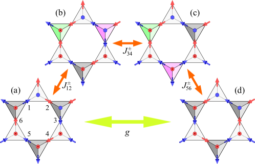
Figure 4: (Color online) An example of quantum tunnelling between two different spin configurations obeying the ice rules, mediated by the virtual excitation of a pair of magnetic monopoles. (a) spin–configuration obeying the ice rules, containing a closed loop of spins, numbered 1…6. (b) excited state containing a pair of magnetic monopoles (green and magnenta tetrahedra). (c) degenerate excited state, in which one of the monopoles has moved. (d) spin–configuration obeying the ice rules, in which the closed loop of spin has been reversed. For the anisotropic exchange model ${\mathcal{H}}_{\sf xxz}$ [Eq. (14)], this process corresponds to 3${}^{\text{rd}}$–order degenerate perturbation in $J_{\pm}$, and leads to the tunneling amplitude $g=12J_{\pm}^{3}/J_{z}^{2}$ [Eq. (16)].

The defining property of spin ice is that at low temperatures spin–configurations obey the “ice rules”, which require that two spins point into, and two spins point out of, every tetrahedron on the lattice. The simplest model leading to the ice rules contains only ferromagnetic exchange $J_{1}<0$, between nearest–neighbour Ising spins. harris97 In this case, all spin configurations obeying the ice rules are degenerate.

The presence of long–range dipolar interactions, and further–neighbour exchanges, lifts this degeneracy, giving rise to the possibility of ordered ground states. However the differences in energy from dipolar interactions alone are smaller than might be excepted, since dipolar interactions are “self-screened” gingras01 ; enjalran04 ; melko04 within spin-ice configurations, decaying as $1/r^{5}$.isakov05 And, as discussed below, there exist a subset of spin-ice configurations, the “chain states”, in which dipolar interactions are even better screened, with interactions decaying exponentially with distance.

II.2 Quantum tunneling between spin-ice states

The minimal change in a spin ice, once quantum effects are taken into account, is the possibility of the system tunneling from one spin–configuration obeying the ice rules to another. Tunnelling matrix elements arise where it is possible to reverse closed loops of spins, with the shortest loop occurring on the hexagonal plaquette shown in Fig. 3.

The natural quantum generalisation of the dipolar spin–ice model is therefore

$$\mathcal{H_{\sf QDSI}}=\mathcal{H}_{\sf dipolar}+\mathcal{H}_{\sf exchange}+\mathcal{H}_{\sf tunneling}\,.$$ (12)

where

$$\mathcal{H}_{\sf tunneling}=-g\sum_{\hexagon}|\!\circlearrowright\rangle\langle\circlearrowleft\!|+|\!\circlearrowleft\rangle\langle\circlearrowright\!|\,.$$ (13)

and the sum upon $\hexagon$ runs over the hexagonal plaquettes of the pyrochlore lattice. In the absence of long–range dipolar or exchange interactions, quantum tunneling of the form $\mathcal{H}_{\sf tunneling}$ [Eq. (13)] is known to stabilize a quantum spin liquid described by a quantum $U(1)$ lattice gauge theory. hermele04 ; banerjee08 ; shannon12 ; benton12

Due to their relative smallness, it is hard even to estimate the strength of quantum tunnelling in spin-ice materials such as Dy₂Ti₂O₇, and the microscopic aspects of the quantum dynamics are only beginning to be understood rau-arXiv ; tomasello-arXiv . However, the form of the tunnelling matrix element $\mathcal{H}_{\sf tunneling}$ [Eq. (13)] is uniquely determined by the ice rules and the geometry of the pyrochlore lattice, so estimates of $g$ can be taken from any quantum model which supports a spin–ice ground state.

The simplest example is an anisotropic exchange model with interactions of “XY” type,

$${\mathcal{H}}_{\sf xxz}=J_{zz}\sum_{\langle ij\rangle}\mathsf{S}_{i}^{z}\mathsf{S}_{j}^{z}-J_{\pm}\sum_{\langle ij\rangle}(\mathsf{S}_{i}^{+}\mathsf{S}_{j}^{-}+\mathsf{S}_{i}^{-}\mathsf{S}_{j}^{+})\,,$$ (14)

with $\mathsf{S}_{i}^{z}$ promoted to a (pseudo) spin-1/2 operator such that

$$[\mathsf{S}_{i}^{+},\mathsf{S}_{j}^{-}]=2\mathsf{S}^{z}_{i}\delta_{ij}\,.$$ (15)

In this case $\mathcal{H}_{\sf tunneling}$ [Eq. (13)] can be derived in degenerate perturbation theory about classical states obeying the ice rules. The tunneling process shown in Fig. 4 can be thought of as the spontaneous creation of a (virtual) pair of magnetic monopoles, which annihilate after one has traversed the hexagon, leading to an effective tunneling

$$g=\frac{12J_{\pm}^{3}}{J_{zz}^{2}}\,.$$ (16)

A more general starting point for describing a quantum spin ice is the anisotropic nearest-neighbour exchange model onoda11 ; savary12-PRL108 ; lee12

$$\mathcal{H}_{\sf S=1/2}= \sum_{\langle ij\rangle}\Big{\{}J_{zz}\mathsf{S}_{i}^{z}\mathsf{S}_{j}^{z}-J_{\pm}(\mathsf{S}_{i}^{+}\mathsf{S}_{j}^{-}+\mathsf{S}_{i}^{-}\mathsf{S}_{j}^{+})$$

$$+J_{\pm\pm}\left[\gamma_{ij}\mathsf{S}_{i}^{+}\mathsf{S}_{j}^{+}+\gamma_{ij}^{*}\mathsf{S}_{i}^{-}\mathsf{S}_{j}^{-}\right]$$

$$+J_{z\pm}\left[\mathsf{S}_{i}^{z}(\zeta_{ij}\mathsf{S}_{j}^{+}+\zeta^{*}_{ij}\mathsf{S}_{j}^{-})+{i\leftrightarrow j}\right]\Big{\}}\,,$$ (17)

where the sum $\langle ij\rangle$ runs over the nearest-neighbour bonds of the pyrochlore lattice; and $\gamma_{ij}$ and $\zeta_{ij}$ are $4\times 4$ complex unimodular matrices encoding the rotations between the local axes $\mathbf{\hat{z}}_{i}$ and the cubic axes of crystal. curnoe08 ; ross11-PRX1

The (pseudo) spin-1/2 model $\mathcal{H}_{\sf S=1/2}$ [Eq. (17)], has been shown to give a quantitative description of spin excitations in both the “quantum spin ice” Yb₂Ti₂O₇ [ross11-PRX1, ] and quantum order-by-disorder system Er₂Ti₂O₇ [savary12-PRL109, ]. The parameterization of $\mathcal{H}_{\sf S=1/2}$ [Eq. (17)], and its mean-field phase diagram have been explored in Refs. [onoda11, ; savary12-PRL108, ; savary13, ; lee12, ]. We will not develop this topic further here, but note that the additional terms, $J_{z\pm}$ and $J_{\pm\pm}$, can also contribute to the tunneling $g$, but do so in higher orders of perturbation theory than $J_{\pm}$ [Eq. (16)].

II.3 Choice of parameters

Like other spin ices, Dy₂Ti₂O₇ is believed to be well–described by the dipolar spin–ice model $\mathcal{H_{\sf DSI}}$ [Eq. (7)], and the values of the parameters $D$ and $J_{k}$ have been estimated by Yavors’kii et al. in Ref. [yavorskii08, ]. In this case, the lattice constant $a=10.124\ \AA$ [fukazawa02, ], and the Dy³⁺ ions have a Landé factor $g_{\sf L}=4/3$ associated with an Ising moment $\langle\mathsf{J}^{z}\rangle=7.40\ \mu_{B}$. It follows from Eq. (10) that

$$D=1.3224\ \text{K}\,.\qquad[\text{Dy${}_{2}$Ti${}_{2}$O${}_{7}$}]$$ (18)

Competing exchange interactions were estimated on the basis of fits of classical Monte Carlo simulation to the structure factor $S({\bf q})$ measured in (diffuse) neutron scattering. Working within the simplifying assumption

$$J_{3c}=J_{3d}=J_{3}\;,\qquad[\text{Ref.~{}{{\cite[citep]{\@@bibref{AuthorsPhrase1Year}{yavorskii08}{\@@citephrase{, }}{}}}}}]$$ (19)

Yavors’kii et al. [yavorskii08, ] find

$$J_{1}= 3.41\ \text{K}\,,$$

$$J_{2}= - 0.14\ \text{K}\,,\qquad[\text{Dy${}_{2}$Ti${}_{2}$O${}_{7}$}]$$ (20)

$$J_{3}= 0.03\ \text{K}\,,$$

For the purposes of this Article, we work with parameters $D$ and $J_{k}$ chosen such that the net effect of the interactions in $\mathcal{H_{\sf DSI}}$ [Eq. (7)] is to enforce the ice–rules constraint. We consider all possible exchanges up to 3${}^{\text{rd}}$–neighbour, as illustrated in Fig. 3, maintaining the distinction $J_{3c}\neq J_{3d}$. However, since $J_{1}$ plays no part in selecting ordered ground states we set $J_{1}\equiv 0$, except where needed for comparison with the finite–temperature properties of real materials.

A further simplication arises since, within spin–configurations obeying the ice rules, the effect of the 3${}^{\text{rd}}$–neighbour exchange $J_{3c}$ is simply to renormalise the 2${}^{\text{nd}}$–neighbour exchange,

$$J_{2}\to J_{2}+3J_{3c}\;,$$ (21)

leaving only $J_{2}$ and $J_{3d}$ as independent parameters. This equivalence is proved in Appendix B.

Mindful of Dy₂Ti₂O₇ [cf. Eq. (II.3)], we will generally assume that $J_{2}$ is the leading form of exchange interaction. And for the purposes of soft–spin mean–field theory [Sec. III], classical Monte Carlo simulation [Sec. V], and quantum Monte Carlo simulation [Sec. VI], we will generally consider ferromagnetic $J_{2}<0$, setting all other exchange interactions to zero.

III Mean–field ground states of dipolar spin ice

Many of the properties of spin-ice materials [denHertog00, ; isakov05, ] can be successfully described using a “soft–spin” mean field theory, in which the “hard–spin” constraint of fixed spin-length

$$({\sf S}^{z}_{i})^{2}=\frac{1}{4}\;,$$ (22)

is relaxed, and spins are treated as continuous variables.

In what follows, we use such a soft–spin mean–field theory to explore the classical ground state–phase diagram of $\mathcal{H_{\sf DSI}}$ [Eq. (7)]. We focus on the competition between long–range dipolar interactions $D$ and second–neighbour exchange $J_{2}$, and construct a mean–field phase diagram as a function of $J_{2}/D$.

The starting point for our mean–field theory is the Fourier transform of the combined dipolar and exchange interactions, $\mathcal{J}^{ab}_{\bf q}$, where the index

$$a,b=0,1,2,3$$ (23)

counts the 4 sites of the tetrahedron $i$ as defined in Eq. (2) (which is the primitive unit cell), with the local axis given by Eq. (6). Following Reimers et al. [reimers91, ], den Hertog et al. [denHertog00, ], and Isakov et al. [isakov05, ], we write

$$\mathcal{H_{\sf DSI}}\approx\overline{\mathcal{H}}_{\sf DSI}=\sum_{\bf q}^{a,b}\mathcal{J}^{ab}_{\bf q}m^{a}_{\bf q}m^{b}_{\bf-q}\;,$$ (24)

where

$$m^{a}_{\bf q}=\frac{1}{\sqrt{N}}\sum_{i\in a}{\sf S}^{z}_{i}e^{i{\bf q}\cdot{\bf r}_{i}}\;,$$ (25)

and similar equations hold for sublattice $b$, $c$, $d$. The contribution to $\mathcal{J}^{ab}_{\bf q}$ from long–range dipolar interactions is determined by an Ewald summation, as described in Ref. [enjalran04, ].

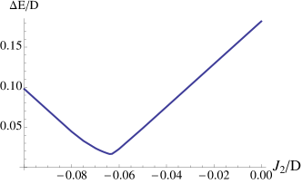
Figure 5: (Color online) Band-width $\Delta E$ [Eq. (29)] of spin-ice states in the presence of long-range dipolar interactions $D$, as a function of second-neighbour exchange $J_{2}<0$, within the soft spin-mean field theory $\overline{\mathcal{H}}_{\sf DSI}$ [Eq. (24)]. For small $|J_{2}|/D$, the competing exchange interaction leads to a reduction in the bandwidth of spin-ice states, which takes on a minimum value for $J_{2}/D=-0.062$.

The eigenvalues of the matrix $\mathcal{J}^{ab}_{\bf q}$,

$$\mathcal{J}_{\bf q}\cdot\boldsymbol{\mathcal{E}}_{\mathbf{q}}^{\mu}=\epsilon_{\mathbf{q}}^{\mu}\boldsymbol{\mathcal{E}}_{\mathbf{q}}^{\mu}\,,$$ (26)

form four dispersing bands $\epsilon_{\mathbf{q}}^{\mu}$, labeled by $\mu$. The eigenvector $\boldsymbol{\mathcal{E}}_{\mathbf{q}_{\sf min}}^{\mu_{\sf min}}$ with the lowest eigenvalue(s)

$$\mathcal{J}_{\bf q}\cdot\boldsymbol{\mathcal{E}}_{\mathbf{q}_{\sf min}}^{\mu_{\sf min}}=\epsilon_{\mathbf{q}_{\sf min}}^{\mu_{\sf min}}\boldsymbol{\mathcal{E}}_{\mathbf{q}_{\sf min}}^{\mu_{\sf min}}\,.$$ (27)

is(are) a ground state of $\overline{\mathcal{H}}_{\sf DSI}$ [Eq. (24)]. As long as the associated eigenvector $\boldsymbol{\mathcal{E}}_{\mathbf{q}_{\sf min}}^{\mu_{\sf min}}$ satisfies the “hard-spin” constraint Eq. (22), this state is also a valid ground state of original dipolar spin–ice model $\mathcal{H_{\sf DSI}}$ [Eq. (7)]. Once this constraint is (re)imposed, the soft–spin approximation becomes equivalent to the well-known Luttinger–Tisza method. luttinger46

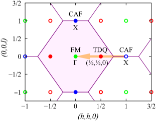
Figure 6: (Color online) Wave vectors associated with ordered ground states in a dipolar spin ice described by $\mathcal{H}_{\sf DSI}$ [Eq. (7)]. The cubic antiferromagnet (CAF) has ordering vector ${\bf Q}^{\sf CAF}=(0,0,1)$ [Eq. (31)], and symmetry–related points [including the (1,1,0)], here labelled “$X$” (blue points). The tetragonal double-Q state (TDQ) has is based on pairs of ordering vectors of the form ${\bf Q}^{\sf TDQ}=\pm(1/2,1/2,0)$ [Eq. (37)], shown with red points. The ferromagnet (FM) has ordering vector ${\bf Q}^{\sf FM}=(0,0,0)$ [Eq. (35)], here labelled “$\Gamma$” (green points). The evolution of the ordering vector within the soft–spin mean field–theory $\overline{\mathcal{H}}_{\sf DSI}$ [Eq. (24)] is shown with an orange arrow.

In the simplest model of a spin–ice, in which only nearest–neighbour interactions are taken into account, there is no unique eigenvector $\boldsymbol{\mathcal{E}}_{\mathbf{q}_{\sf min}}^{\mu_{\sf min}}$ with a minimum energy. Instead the two lowest-lying eigenstates form “flat” bands with

$$\epsilon_{\mathbf{q}}^{\sf 1}=\epsilon_{\mathbf{q}}^{\sf 2}\equiv 0.$$ (28)

These bands describe the (extensively degenerate) set of spin configurations which obey the two-in two-out “ice rules” [denHertog00, ; melko01, ; isakov05, ].

The degeneracy of the spin–ice configurations is lifted by long–range dipolar interactions, causing these flat bands to acquire a dispersion. However dipolar interactions, despite being long-range, are effectively “self-screened” within the spin-ice states, denHertog00 a fact known as “projective equivalence” [isakov05, ]. The overall bandwidth of spin-ice states in the presence of dipolar interactions

$$\Delta E=\text{Max}(\epsilon_{\mathbf{q}}^{\sf 1},\epsilon_{\mathbf{q}}^{\sf 2})-\text{Min}(\epsilon_{\mathbf{q}}^{\sf 1},\epsilon_{\mathbf{q}}^{\sf 2})\approx 0.17D$$ (29)

and is significantly smaller than the bare scale of dipolar interactions $D$. None the less, dipolar interactions do select an ordered ground state, as described below.

We now turn to question of finding the ground state of $\mathcal{H}_{\sf DSI}$ [Eq. (7)] as function of $J_{2}/D$. Within the soft-spin approximation $\overline{\mathcal{H}}_{\sf DSI}$ [Eq. (24)], for $J_{2}<0$, there are three distinct regimes, corresponding to different ordering vectors

$${\bf q}_{\sf min}=\frac{2\pi}{a}\;{\bf Q}_{\sf min}\;,$$ (30)

where $a$ is the (cubic) lattice spacing, and ordering vectors are measured relative to the usual, cubic, crystallographic coordinates. We consider each of these regimes in turn, below.

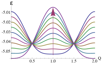
Figure 7: (Color online) Evolution of the dispersion of lowest-lying eigenvalue of $\overline{\mathcal{H}}_{\sf DSI}$ [Eq. (24)], as a function of second-neighbour exchange $J_{2}<0$, for wave vector ${\bf Q}=(Q,Q,0)$. For $J_{2}/D=-0.057$, (blue curve) the minimum of the dispersion is found at ${\bf Q}^{\sf CAF}=\left(1,1,0\right)$. For $J_{2}/D=-0.08$, (purple curve) the minimum of the dispersion is found at ${\bf Q}^{\sf FM}=\left(0,0,0\right)$. The direction of decreasing $J_{2}/D$ is shown with an arrow. The mean field energy at $Q=1/2$ and $3/2$ does not depend on $J_{2}/D$, this is the origin of the line crossings.

Table 1: Chain–based ordered ground states of dipolar spin ice, $\mathcal{H_{\sf QDSI}}$ [Eq. (12)]. The ordering wave vector $\mathbf{Q}$, [cf. Fig. 6], is measured in reciprocal lattice units [cf. Eq. (30)]. Also listed are the corresponding spin eigenvector [cf. Eq. (26)], the chain directions associated with each eignvector, and the degeneracy of the state. The cubic antiferromagnet (CAF), tetragonal double–Q (TDQ) and ferromagnet (FM) are all found in classical treatments of dipolar spin ice [Sec III,IV,V]. In contrast, the orthorhombic zig-zag (OZZ) is only stabilised by quantum effects [Sec. VI]. All four ordered states are illustrated in Fig. 2.

state	ordering wavevector ${\bf Q}$	eigenvectors $\boldsymbol{\mathcal{E}}_{\mathbf{Q}}$	chain directions	degen.	figure
	$\begin{array}[]{c}(1,0,0)\end{array}$	$\begin{array}[]{rl}\frac{1}{2}(-1)^{j}\left(1,-1,0,0\right),&j=1,2\\ \frac{1}{2}(-1)^{j^{\prime}}\left(0,0,1,-1\right),&j^{\prime}=1,2\end{array}$	$\begin{array}[]{c}[0,1,1]\\ {}[0,1,\bar{1}]\end{array}$	4	Fig. 2(a)
CAF	$\begin{array}[]{c}(0,1,0)\end{array}$	$\begin{array}[]{rl}\frac{1}{2}(-1)^{j}\left(1,0,-1,0\right),&j=1,2\\ \frac{1}{2}(-1)^{j^{\prime}}\left(0,1,0,-1\right),&j^{\prime}=1,2\end{array}$	$\begin{array}[]{c}[1,0,1]\\ {}[1,0,\bar{1}]\end{array}$	4
	$\begin{array}[]{c}(0,0,1)\end{array}$	$\begin{array}[]{rl}\frac{1}{2}(-1)^{j}\left(1,0,0,-1\right),&j=1,2\\ \frac{1}{2}(-1)^{j^{\prime}}\left(0,1,-1,0\right),&j^{\prime}=1,2\end{array}$	$\begin{array}[]{c}[1,1,0]\\ {}[1,\bar{1},0]\end{array}$	4
	$\begin{array}[]{c}\left(0,\frac{1}{2},-\frac{1}{2}\right)\\ \left(0,\frac{1}{2},\frac{1}{2}\right)\end{array}$	$\begin{array}[]{rl}\frac{1}{\sqrt{2}}e^{i(2j+1)\pi/4}\left(1,-1,0,0\right),&j=1,2,3,4\\ \frac{1}{\sqrt{2}}e^{i(2j^{\prime}+1)\pi/4}\left(0,0,1,-1\right),&j^{\prime}=1,2,3,4\end{array}$	$\begin{array}[]{c}[0,1,1]\\ {}[0,1,\bar{1}]\end{array}$	16	Fig. 2(b)
TDQ	$\begin{array}[]{c}\left(\frac{1}{2},0,-\frac{1}{2}\right)\\ \left(\frac{1}{2},0,\frac{1}{2}\right)\end{array}$	$\begin{array}[]{rl}\frac{1}{\sqrt{2}}e^{i(2j+1)\pi/4}\left(1,0,-1,0\right),&j=1,2,3,4\\ \frac{1}{\sqrt{2}}e^{i(2j^{\prime}+1)\pi/4}\left(0,1,0,-1\right),&j^{\prime}=1,2,3,4\end{array}$	$\begin{array}[]{c}[1,0,1]\\ {}[1,0,\bar{1}]\end{array}$	16
	$\begin{array}[]{c}\left(\frac{1}{2},-\frac{1}{2},0\right)\\ \left(\frac{1}{2},\frac{1}{2},0\right)\end{array}$	$\begin{array}[]{rl}\frac{1}{\sqrt{2}}e^{i(2j+1)\pi/4}\left(1,0,0,-1\right),&j=1,2,3,4\\ \frac{1}{\sqrt{2}}e^{i(2j^{\prime}+1)\pi/4}\left(0,1,-1,0\right),&j^{\prime}=1,2,3,4\end{array}$	$\begin{array}[]{c}[1,1,0]\\ {}[1,\bar{1},0]\end{array}$	16
	$\begin{array}[]{c}(0,0,0)\\ {}\hfil\end{array}$	$\begin{array}[]{c}\pm\frac{1}{2}\left(1,-1,-1,1\right)\\ {}\hfil\end{array}$	$\begin{array}[]{c}[0,1,1]\;\&\;[0,1,\bar{1}]\\ \text{}[1,0,1]\;\&\;[1,0,\bar{1}]\end{array}$	$\begin{array}[]{c}2\\ {}\hfil\end{array}$	$\begin{array}[]{c}\text{Fig.~{}\ref{fig:ordered.phases}(c)}\\ {}\hfil\end{array}$
FM	$\begin{array}[]{c}(0,0,0)\\ {}\hfil\end{array}$	$\begin{array}[]{c}\pm\frac{1}{2}\left(1,-1,1,-1\right)\\ {}\hfil\end{array}$	$\begin{array}[]{c}[0,1,1]\;\&\;[0,1,\bar{1}]\\ \text{}[1,1,0]\;\&\;[1,\bar{1},0]\end{array}$	$\begin{array}[]{c}2\\ {}\hfil\end{array}$
	$\begin{array}[]{c}(0,0,0)\\ {}\hfil\end{array}$	$\begin{array}[]{c}\pm\frac{1}{2}\left(1,1,-1,-1\right)\\ {}\hfil\end{array}$	$\begin{array}[]{c}[1,0,1]\;\&\;[1,0,\bar{1}]\\ \text{}[1,1,0]\;\&\;[1,\bar{1},0]\end{array}$	$\begin{array}[]{c}2\\ {}\hfil\end{array}$
	$\begin{array}[]{c}\left(0,\frac{1}{2},-\frac{1}{2}\right)\\ \left(1,0,0\right)\end{array}$	$\begin{array}[]{rl}\frac{1}{\sqrt{2}}e^{i(2j+1)\pi/4}\left(1,-1,0,0\right),&j=1,2,3,4\\ \frac{1}{2}(-1)^{j^{\prime}}\left(0,0,1,-1\right),&j^{\prime}=1,2\end{array}$	$\begin{array}[]{c}[0,1,1]\\ {}[0,1,\bar{1}]\end{array}$	8	Fig. 2(d)
	$\begin{array}[]{c}\left(1,0,0\right)\\ \left(0,\frac{1}{2},\frac{1}{2}\right)\end{array}$	$\begin{array}[]{rl}\frac{1}{2}(-1)^{j}\left(1,-1,0,0\right),&j=1,2\\ \frac{1}{\sqrt{2}}e^{i(2j^{\prime}+1)\pi/4}\left(0,0,1,-1\right),&j^{\prime}=1,2,3,4\end{array}$	$\begin{array}[]{c}[0,1,1]\\ {}[0,1,\bar{1}]\end{array}$	8
OZZ	$\begin{array}[]{c}\left(\frac{1}{2},0,-\frac{1}{2}\right)\\ \left(0,1,0\right)\end{array}$	$\begin{array}[]{rl}\frac{1}{\sqrt{2}}e^{i(2j+1)\pi/4}\left(1,0,-1,0\right),&j=1,2,3,4\\ \frac{1}{2}(-1)^{j^{\prime}}\left(0,1,0,-1\right),&j^{\prime}=1,2\end{array}$	$\begin{array}[]{c}[1,0,1]\\ {}[1,0,\bar{1}]\end{array}$	8
	$\begin{array}[]{c}\left(0,1,0\right)\\ \left(\frac{1}{2},0,\frac{1}{2}\right)\end{array}$	$\begin{array}[]{rl}\frac{1}{2}(-1)^{j}\left(1,0,-1,0\right),&j=1,2\\ \frac{1}{\sqrt{2}}e^{i(2j^{\prime}+1)\pi/4}\left(0,1,0,-1\right),&j^{\prime}=1,2,3,4\end{array}$	$\begin{array}[]{c}[1,0,1]\\ {}[1,0,\bar{1}]\end{array}$	8
	$\begin{array}[]{c}\left(\frac{1}{2},-\frac{1}{2},0\right)\\ \left(0,0,1\right)\end{array}$	$\begin{array}[]{rl}\frac{1}{\sqrt{2}}e^{i(2j+1)\pi/4}\left(1,0,0,-1\right),&j=1,2,3,4\\ \frac{1}{2}(-1)^{j^{\prime}}\left(0,1,-1,0\right),&j^{\prime}=1,2\end{array}$	$\begin{array}[]{c}[1,1,0]\\ {}[1,\bar{1},0]\end{array}$	8
	$\begin{array}[]{c}\left(0,0,1\right)\\ \left(\frac{1}{2},\frac{1}{2},0\right)\end{array}$	$\begin{array}[]{rl}\frac{1}{2}(-1)^{j}\left(1,0,0,-1\right),&j=1,2\\ \frac{1}{\sqrt{2}}e^{i(2j^{\prime}+1)\pi/4}\left(0,1,-1,0\right),&j^{\prime}=1,2,3,4\end{array}$	$\begin{array}[]{c}[1,1,0]\\ {}[1,\bar{1},0]\end{array}$	8

III.1 Cubic antiferromagnet (CAF)

For purely dipolar interactions ${\mathcal{H}}_{\sf dipolar}$ [Eq. (8)], the minimum of the lowest lying (nearly-flat) band $\epsilon_{\mathbf{q}}^{\mu}$ lies at

$${\bf Q}^{\sf CAF}=\left(0,0,1\right)$$ (31)

— the X point in Fig. 6, and two other wave vectors related by cubic symmetry.

The spectrum of $\overline{\mathcal{H}}_{\sf DSI}$ [Eq. (24)] is doubly–degenerate at these wavevectors, with associated eigenvectors

$$\boldsymbol{\mathcal{E}}_{\mathbf{Q}^{\sf CAF}}^{1^{\prime}} = \frac{1}{\sqrt{2}}\left(1,0,0,-1\right)\,,$$

$$\boldsymbol{\mathcal{E}}_{\mathbf{Q}^{\sf CAF}}^{2^{\prime}} = \frac{1}{\sqrt{2}}\left(0,1,-1,0\right)\,.$$ (32)

These eigenvectors satisfy the hard–spin constraint Eq. (22), and correspond to the CAF — an antiferromagnet ground state with cubic symmetry, studied extensively by Melko et al. [melko01, ]. Competing second-neighbour exchange, $J_{2}<0$, leads a reduction in the bandwidth of spin-ice configurations $\Delta E$, as illustrated in Fig. 5. However the CAF remains a mean-field ground state for

$$J_{2}/D>-0.057(1)\;,$$ (33)

where the bracket indicates the uncertainty in the final digit.

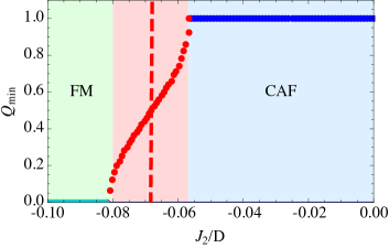
Figure 8: (Color online) Evolution of the mean–field ordering wave vector, ${\bf Q}_{\sf min}=(Q,Q,0)$ as a function of second–neighbour exchange $J_{2}<0$, within a dipolar spin ice described by the soft–spin mean–field theory $\overline{\mathcal{H}}_{\sf DSI}$ [Eq. (24)]. ${\bf Q}_{\sf min}$ interpolates smoothly from ${\bf Q}^{\sf CAF}=(1,1,0)$ [labelled $X$ in Fig. (6)], through incommensurate values, to ${\bf Q}^{\sf FM}=(0,0,0)$, [labelled $\Gamma$ in Fig. (6)]. The wave vectors associated with the tetragonal double-Q (TDQ) state, including ${\bf Q}^{\sf TDQ}=(1/2,1/2,0)$ [cf. Table 1], occur for $J_{2}/D=-0.068$ (red dashed line), within the incommensurate region.

The CAF ground state is illustrated in Fig. 2(a). (An equivalent animated figure is provided in the supplemental materials). It has the same 16–site cubic unit cell as the pyrochlore lattice. Once time–reversal symmetry is taken into account, each of the three possible ordering vectors ${\bf Q}^{\sf CAF}$ contributes four possible ground states, leading to an overall 12–fold degeneracy.

In Fig. 2(a), the CAF is shown within a tetragonal 32–site cell, aligned with the $[110]$ and $[1\overline{1}0]$ axes of the lattice. Plotted in this way, it becomes clear that the CAF is built of alternating chains of spins (coloured blue and red, respectively), running parallel to the $[110]$ and $[1\overline{1}0]$ axes (green and yellow lines, respectively), corresponding to the $\boldsymbol{\mathcal{E}}_{\mathbf{Q}^{\sf CAF}}^{1^{\prime}}$ and $\boldsymbol{\mathcal{E}}_{\mathbf{Q}^{\sf CAF}}^{2^{\prime}}$ eigenvectors [Eqs. (32)], respectively. Each of these chains has a net ferromagnetic polarisation. However, the polarisation of the chains rotates between the different $[001]$ planes of the lattice, to give a state with no net magnetisation.

III.2 Incommensurate states and tetragonal double–Q (TDQ) order

In the intermediate parameter range

$$-0.080<J_{2}/D<-0.057$$ (34)

the dispersion of lowest-lying eigenvalue of $\overline{\mathcal{H}}_{\sf DSI}$, Eq. (24), evolves smoothly from a band with a minimum at ${\bf Q}^{\sf CAF}$ [Eq. (31)] to band with a minimum at

$${\bf Q}^{\sf FM}=(0,0,0)\,,$$ (35)

as illustrated in Fig. 7. The corresponding mean-field ordering wave vector, $\mathbf{Q}_{\sf min}$, interpolates between ${\bf Q}^{\sf CAF}$ and ${\bf Q}^{\sf FM}$, following the path shown in Fig. 6.

In general, the eigenvectors $\boldsymbol{\mathcal{E}}_{\mathbf{Q}_{\sf min}}^{\mu}$ in this range of $J_{2}/D$ [Eq. (34)] do not satisfy the hard–spin constraint Eq. (22). However a special case, occurring for

$$J_{2}/D=-0.068(1)\;,$$ (36)

is the commensurate wavevector

$${\bf Q}^{\sf TDQ} = \left(\frac{1}{2},\frac{1}{2},0\right)\;.$$ (37)

In this case, it is possible to construct to linear combinations of pairs of the 12 eigenvectors $\boldsymbol{\mathcal{E}}_{\mathbf{Q}^{\sf TDQ}}^{\mu}$, listed in Table 1, which do satisfy the hard-spin constraint. These correspond to the 48–fold degenerate, tetragonal, double–Q state (TDQ) illustrated in Fig. 2(b). (An equivalent animated figure is provided in the supplemental materials).

Close examination of Fig. 2(b) reveals that the TDQ state, like the CAF, is built of alternating chains of spins, running parallel to the $[110]$ and $[1\overline{1}0]$ axes. Each alternating chain has a net ferromagnetic polarisation. However the sense of this polarisation alternates between neighbouring chains, to give a state with no net magnetisation.

To rule out the possibility of other mean–field ground states in this parameter range, we have carried out a search of all possible multiple–Q states of the form

$$\Psi^{a}(\mathbf{r}_{i,a}) = \sum_{\eta}\left[z^{a}_{\eta}e^{i\mathbf{q}_{\sf min}^{\eta}\cdot\mathbf{r}_{i,a}}+\text{c.c.}\right]\;.$$ (38)

where $z^{a}_{\eta}$ is a 4–component vector proportional to $\boldsymbol{\mathcal{E}}^{\mu}_{\mathbf{Q}_{\sf min}^{\eta}}$, and the sum $\sum_{\eta}$ runs over the six distinct mean–field ordering wave vectors given in Table 1. We find that the only solutions $\Psi^{a}(\mathbf{r}_{i,a})$ which satisfy the hard–spin constraint [Eq. (22)], are those corresponding to the TDQ states.

III.3 Ferromagnet (FM)

Finally, for parameters

$$J_{2}/D<-0.080(1)$$ (39)

we find $\mathbf{Q}_{\sf min}$ equal to ${\bf Q}^{\sf FM}$ [Eq. (35)], and eigenvectors have unique solutions of the simple “two–in, two–out” form

$$\boldsymbol{\mathcal{E}}_{\mathbf{Q}^{\sf FM}}^{\mu_{\sf min}} = \frac{1}{2}\left(1,1,-1,-1\right)\;.$$ (40)

There are three such eigenvectors up to time reversal and they are listed in Table 1. These eigenvectors trivially satisfy the hard-spin constraint Eq. (22), and correspond to a simple ferromagnet (FM) in which all tetrahedra have the same spin configuration. Since there are six possible “two–in, two–out” spin configurations for a single tetrahedron, the FM is six–fold degenerate.

The FM state is illustrated in Fig. 2(c). (An equivalent animated figure is provided in the supplemental materials). Once again, the FM can be seen to be built of alternating chains of spins, running parallel to the $[110]$ and $[1\overline{1}0]$ axes. However, unlike the CAF or TDQ state, all chains parallel to $[110]$ or $[1\overline{1}0]$ have the same polarisation, and as a result the FM has a net magnetization parallel to the $[100]$ axis.

IV Mapping to an effective triangular–lattice Ising model

The mean–field treatment of dipolar spin ice, developed in Sec. III, reveals three different ordered ground states as a function of second neighbour exchange $J_{2}<0$ — a cubic antiferromagnet (CAF), a tetragonal double–Q (TDQ) state, and a cubic ferromagnet (FM). These three ordered states have a striking common feature — they are all built of alternating chains of spins.

Numerical simulations, described in Sec. V, confirm that the CAF, TDQ and FM states are indeed the classical ground states of $\mathcal{H_{\sf DSI}}$ [Eq. (7)] for $J_{2}<0$. However neither these simulations, nor the mean–field theory, explain why ordered ground states should be built of alternating chains of spins. Moreover, the fact that three different ground states are found within such a small range of $J_{2}/D$ [cf. Fig. 8] suggests that ground state order might also be very sensitive to third neighbour exchanges $J_{3c}$ and $J_{3d}$, not treated in Sec. III.

Taken together, these results suggest that a new ordering principle is at work in dipolar spin ice at low temperatures. In what follows we identify this ordering principle, showing how long–range dipolar interactions between alternating chains of spins can be described by an effective Ising model on an anisotropic triangular lattice, with only weak, short–ranged interactions. The extreme sensitivity of the ground state dipolar spin–ice to competing exchange interactions is shown to follow from the exponential–screening of dipolar interactions within such “chain states”.

We develop, below, the classical, ground-state phase diagram of this Ising model, and show how it can be used to determine the ordered phases of a dipolar spin ice with competing further-neighbour exchange.

IV.1 Effective Ising model

Spin ice is not the only material where long–range interactions arise within an ice–like manifold of states. Another example, famously studied by Anderson is the charged ordered system magnetite, Fe₃O₄. In a seminal paper, anderson56 Anderson argued that Fe²⁺ and Fe³⁺ ions, occupying the sites of a pyrochlore lattice in magnetite, could be equated with the hydrogen bonds in water ice. The tendency to charge order means that they are subject to the same “ice rule”, namely that there should be exactly two Fe²⁺ and two Fe³⁺ in every tetrahedron in the lattice. The degeneracy of these ice–like, locally charge–ordered states is lifted by long–range Coulomb interactions between the Fe²⁺ and Fe³⁺ ions. anderson56 ; mcclarty14 At first sight, evaluating the effect of these long–range interactions is a very challenging problem. However, as Anderson realised, the particular geometry of pyrochlore lattice leads to a significant simplification.

The pyrochlore lattice can be broken down into sites on two sets of chains, running parallel to $[110]$ and $[1\overline{1}0]$, with a tetrahedron at every point where two perpendicular chains cross. States satisfying the “ice rule” can be constructed by populating these chains with alternating Fe²⁺ and Fe³⁺ ions. These chains of alternating charges are charge–neutral objects (relative to the average valence of Fe^2.5+), and so interact only weakly. Moreover, it follows from the symmetry of the lattice that interactions between perpendicular chains vanish. What remains are two, independent, sets of weakly–interacting chains, whose low–energy states can be described by an Ising variable on a triangular lattice. The two states of the Ising variable stand for the two possible states of the ferromagnetic chains.

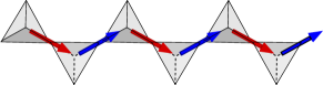
(a)

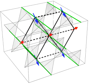
(b)

Figure 9: (Color online) Mapping from spin-ice states to the anisotropic Ising model on a triangular lattice. (a) Alternating chain of spins, with net ferromagnetic magnetisation. (b) Pyrochlore lattice, showing how chains parallel to $[110]$ form a triangular lattice.

All of the same considerations apply in spin-ice, where spins interact through long–range dipolar interactions, and the alternating charges are replaced by alternating spins (blue and red arrows in Fig. 9), to form ferromagnetic chains. We consider the two sets of chains parallel to the $[1,1,0]$ and $[1,\overline{1},0]$ directions. In units of

$$r_{1}^{\prime}=\frac{a}{4}=\frac{r_{1}}{\sqrt{2}}$$ (41)

[cf. Eq. (9)], the coordinates of the spins on these chains are given by

$$(n+l,-n+l,2m) \quad(\text{chain}\parallel[1,1,0])\,,$$ (42)

$$(n+1+l,n-l,2m+1) \quad(\text{chain}\parallel[1,\overline{1},0])\,,$$

where

$$l=-\infty\ldots-2,-1,0,1,2,\ldots\infty$$ (43)

counts the spins on a given chain, while the integers $m$ and $n$ (such that $m+n$ is even) determine the chain in question and at the same time, for $l=0$, define the sites of an anisotropic triangular lattice (solid and dashed black lines in Fig. 9), with coordinates

$$\boldsymbol{\delta} = (\delta_{1},\delta_{2})\equiv(\delta_{1},-\delta_{1},\sqrt{2}\delta_{2})=(n,-n,2m)$$ (44)

$$\qquad\qquad\qquad\qquad(\text{chain}\parallel[1,1,0])\,.$$

In units of $r_{1}$ [Eq. (9)], projecting onto a $(1,1,0)$ plane, these correspond to a lattice with primitive lattice vectors

$$\mathbf{a}=(2,0)\quad,\quad\mathbf{b}=(1,\sqrt{2})\;.$$ (45)

An exactly equivalent triangular lattice can be assigned to chains parallel to $[1,\overline{1},0]$. We note that the local easy–axis of the spins within each of these triangular lattices points in one of two directions, and is the same for all even (odd) $n$ — cf. Fig. 9.

Following Anderson, anderson56 we now consider the specific case of states composed of alternating chains of spins, running parallel to $[1,1,0]$ and $[1,\overline{1},0]$, with net ferromagnetic polarisation. Such states automatically satisfy the “ice rules”, and so are candidates as ground states in a spin ice. Moreover, dipolar interactions between orthogonal ferromagnetic spin–chains vanish by symmetry (by analogy to the charge problem mentioned above), while interactions between parallel chains can be described by an effective Ising model

$${\mathcal{H}}^{\sf 2D}_{\sf Ising} = \frac{1}{2}\sum_{\boldsymbol{\rho},\boldsymbol{\delta}}K_{\boldsymbol{\delta}}\,\sigma_{\boldsymbol{\rho}}\ \sigma_{\boldsymbol{\rho}+\boldsymbol{\delta}}\,,$$ (46)

where the sum $\sum_{\boldsymbol{\rho},\boldsymbol{\delta}}$ runs over all pairs of sites within the triangular lattice defined by Eq. (44), and

$$\sigma_{\boldsymbol{\rho}}\equiv 2\sf\mathsf{S}^{z}_{\boldsymbol{\rho}}=\pm 1\;,$$ (47)

is the Ising variable characterising the state of a given ferromagnetic chain.

What remains is to determine the strength of the interaction $K_{\boldsymbol{\delta}}$ [Eq. (46)] between parallel chains. These will have contributions from both long–range dipolar interaction ${\mathcal{H}}_{\sf dipolar}$ [Eq. (8)], and exchange interactions ${\mathcal{H}}_{\sf exchange}$ [Eq. (11)]. Just as in the problem of charge–order, anderson56 the contribution of the long range dipolar interactions can be calculated through a Madelung sum. We start by considering the dipolar interaction between a test spin at $\boldsymbol{\delta}=(0,0)$ and a chain $\parallel[1,1,0]$, at position $\boldsymbol{\delta}=(\delta_{1},\delta_{2})$

$$K_{\boldsymbol{\delta}}=\frac{D}{3}\sum_{l=-\infty}^{\infty} \left[(-1)^{l}\frac{\left(\delta_{1}^{2}-2\delta_{2}^{2}+l^{2}\right)}{\left(\delta_{1}^{2}+\delta_{2}^{2}+l^{2}\right)^{5/2}}\right.$$

$$\quad\left.+2(-1)^{\delta_{1}}\frac{\left(\delta_{1}^{2}+\delta_{2}^{2}-2l^{2}\right)}{\left(\delta_{1}^{2}+\delta_{2}^{2}+l^{2}\right)^{5/2}}\right]\,,$$ (48)

where the coordinates of the sites on the chain are given by

$$(n+l,-n+l,2m)=(\delta_{1}+l,\delta_{1}-l,\sqrt{2}\delta_{2})\;,$$

The term with alternating sign comes from the alternating spin components perpendicular to the chain, while the uniform term comes from the spin components parallel to the chain.

Table 2: Interactions $K_{\boldsymbol{\delta}}$ of the extended Ising model ${\mathcal{H}}^{\sf 2D}_{\sf Ising}$ [Eq. (46)], written in terms of the microscopic parameters of $\mathcal{H_{\sf DSI}}$ [Eq. (7)]. The contribution of the long-range dipolar interactions $\mathcal{H}_{\sf dipolar}$ [Eq. (8)] shows exponential decay as a function of distance $|{\boldsymbol{\delta}}|$.

$K_{\boldsymbol{\delta}}$	$|\boldsymbol{\delta}|$	${\mathcal{H}}_{\sf dipolar}$	${\mathcal{H}}_{\sf exchange}$
$K_{(1,\sqrt{2})}$	$\sqrt{3}$	$-0.0227426D$	$-J_{2}/3-J_{3c}-J_{3d}$
$K_{(2,0)}$	$2$	$\phantom{-}0.0021957D$	$J_{3d}$
$K_{(0,2\sqrt{2})}$	$2\sqrt{2}$	$-0.0008443D$
$K_{(3,\sqrt{2})}$	$\sqrt{11}$	$-0.0000178D$
$K_{(2,-2\sqrt{2})}$	$2\sqrt{3}$	$-0.0000649D$
$K_{(1,3\sqrt{2})}$	$\sqrt{19}$	$-0.0000051D$
$K_{(4,0)}$	$4$	$\phantom{-}0.0000013D$

Evaluating the sum in Eq. (48) numerically, we find that the interchain couplings $K_{\boldsymbol{\delta}}$ are very small, and decay very rapidly, with the first few interactions given by

$$K_{(1,\sqrt{2})} =-0.0227D\;,$$

$$K_{(2,0)} =\phantom{-}0.0022D\;,$$ (49)

$$K_{(0,2\sqrt{2})} =-0.0008D\;.$$

Interactions up to 7${}^{\text{th}}$–neighbour, including the contribution of ${\mathcal{H}}_{\sf exchange}$ [Eq. (11)], are listed in Table 2.

In fact, $K_{\boldsymbol{\delta}}$ decays exponentially with distance, as can be seen from Fig. 10, where interactions are plotted for the two main lattice directions, $(0,\delta_{2})$ and $(\delta_{1},0)$. The origin of this exponential decay lies in the alternation of the spins, and can be understood by converting the sums on $l$ in Eq. (48) into integrals, using Fourier representations of the Dirac delta function :

$$\sum_{l=-\infty}^{\infty}f(l) =\sum_{q=-\infty}^{\infty}\int\limits_{-\infty}^{\infty}dl\;f(l)\cos 2ql\pi\;,$$ (50a)

$$\sum_{l=-\infty}^{\infty}(-1)^{l}f(l) =\sum_{q=-\infty}^{\infty}\int\limits_{-\infty}^{\infty}dl\;f(l)\cos(2q+1)l\pi\;.$$ (50b)

Doing so, we obtain

$$K_{\boldsymbol{\delta}}= \frac{D}{3}\sum_{q=-\infty}^{\infty}\int\limits_{-\infty}^{\infty}dl\left[\frac{\left(\delta_{1}^{2}-2\delta_{2}^{2}+l^{2}\right)}{\left(\delta_{1}^{2}+\delta_{2}^{2}+l^{2}\right)^{5/2}}\cos(2q+1)l\pi\right.$$

$$\left.+2(-1)^{\delta_{1}}\frac{\left(\delta_{1}^{2}+\delta_{2}^{2}-2l^{2}\right)}{\left(\delta_{1}^{2}+\delta_{2}^{2}+l^{2}\right)^{5/2}}\cos 2ql\pi\right]\,.$$ (51)

The leading contribution to $K_{\boldsymbol{\delta}}$ comes from the first term in Eq. (51) with $q=-1$ and $q=0$, which decays exponentially with distance :

$$\frac{K_{\boldsymbol{\delta}}}{D}\approx \frac{2}{3}\int_{-\infty}^{\infty}dl\,\frac{\left(\delta_{1}^{2}-2\delta_{2}^{2}+l^{2}\right)}{\left(\delta_{1}^{2}+\delta_{2}^{2}+l^{2}\right)^{5/2}}\cos\pi l$$

$$= \frac{4\pi}{3\delta}K_{1}(\pi\delta)-\frac{4\pi^{2}\delta_{2}^{2}}{3\delta^{2}}K_{2}(\pi\delta)$$

$$\approx -\frac{2\sqrt{2}}{3}\left[\pi^{2}\left(\frac{\delta_{2}}{\delta}\right)^{2}\delta^{-1/2}-\pi\delta^{-3/2}+\cdots\right]e^{-\pi\delta}\;,$$ (52)

where $K_{1}(x)$ and $K_{2}(x)$ are modified Bessel functions of the second kind and

$$\delta=\sqrt{\delta_{1}^{2}+\delta_{2}^{2}}\;.$$ (53)

The neglected integrals decay as $e^{-2\pi\delta}$ or faster with the distance (more precisely, the integral with $\cos pl\pi$ decays as $e^{-p\pi\delta}$).

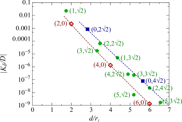
Figure 10: (Color online) Exponential decay of dipolar contributions to the interchain interaction $K_{\boldsymbol{\delta}}$, as a function of the distance between the chains $d/r_{1}=\sqrt{\delta_{1}^{2}+\delta_{2}^{2}}$, where $\boldsymbol{\delta}=(\delta_{1},\delta_{2})$, and $r_{1}$ is defined by Eq. (9). Interactions are measured in units of $D$ [cf. Eq. (10)]. The family of exchanges $K_{(0,\delta_{2})}$ are shown with blue squares, while those for $K_{(\delta_{1},0)}$ are shown with red diamonds. Dashed lines of the same color show the corresponding asymptotic expressions Eqs. (54) and (55). Exchanges for general $(\delta_{1},\delta_{2})$ are plotted as green circles. Interactions denoted with solid symbols are ferrromagnetic ($K_{\boldsymbol{\delta}}<0$); interactions denoted with open symbols are antiferrromagnetic ($K_{\boldsymbol{\delta}}>0$).

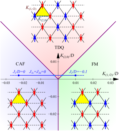
Figure 11: Phase diagram of the extended Ising model ${\mathcal{H}}^{\sf 2D}_{\sf Ising}$ [Eq. (46)], as a function of the leading interchain interactions $K_{(1,\sqrt{2})}$ and $K_{(2,0)}$. In this model, each Ising spin $\sigma_{{\bf r}}$ corresponds to a chain of alternating spins in a dipolar spin–ice described by $\mathcal{H_{\sf DSI}}$ [Eq. (7)], with parameters $K_{\boldsymbol{\delta}}$ given in Table 2. Three ordered ground states are found, a cubic antiferromagnet (CAF), a tetragonal double–Q state (TDQ) and a ferromagnet (FM), illustrated in Fig. 2. The parameters estimated by Ya’vorskii et al. [yavorskii08, ] place Dy₂Ti₂O₇ in the CAF phase. The parameters considered in soft–spin mean–field theory [Sec. III], classical Monte Carlo simulation [Sec. V], and quantum Monte Carlo simulation [Sec. VI], are shown with blue line.

It follows that the assymptotic form of $K_{\boldsymbol{\delta}}$ at large distances is given by

$$K_{(0,\delta_{2})}/D \approx -\frac{\pi^{2}}{3}2^{3/2}\delta_{2}^{-1/2}e^{-\pi\delta_{2}}\;,$$ (54)

$$K_{(\delta_{1},0)}/D \approx \phantom{-}\frac{\pi}{3}2^{3/2}\delta_{1}^{-3/2}e^{-\pi\delta_{1}}\,.$$ (55)

These functions are plotted as dashed lines in Fig. 10.

IV.2 Ground–state phase diagram

Finding the ground state of the dipolar spin–ice model, $\mathcal{H_{\sf DSI}}$ [Eq. (7)], is a daunting task, combining the geometric frustration of the pyrochlore lattice, with long–range interactions and competing exchanges. siddharthan-arXiv ; melko01 ; yavorskii08 In contrast, finding the ground state of the effective two–dimensional Ising model ${\mathcal{H}}^{\sf 2D}_{\sf Ising}$ [Eq. (46)], describing chain states, is relatively easy. In this case, all interactions are short–ranged, and the frustration of the triangular lattice Wannier1950 is lifted by the anisotropy of the leading interactions, $K_{(1,\sqrt{2})}$ and $K_{(2,0)}$. However since dipolar interactions are suppressed by two orders of magnitude within chain state — cf. Table 2 — the behaviour of the model is very sensitive to competing exchange.

Since nearest–neighbour interactions dominate, the ground—state phase diagram of ${\mathcal{H}}^{\sf 2D}_{\sf Ising}$ [Eq. (46)] can be found by examining spin–configurations on the elementary unit of the lattice, a triangle. The resulting phase diagram is shown in Fig. 11, with the parameter set considered in Sec. III shown as a blue line. This phase diagram contains the same three ordered “chain states” as are found in mean–field theory [cf. Table 1] :

1. A cubic antiferromagnet (CAF), with energy per triangle

   $$E^{\sf CAF}_{\triangle}=2K_{(1,\sqrt{2})}+K_{(2,0)}\;.$$ (56)

2. A tetragonal, double-q state (TDQ) with energy per triangle

   $$E^{\sf TDQ}_{\triangle}=-K_{(2,0)}\;.$$ (57)

3. A cubic ferromagnet (FM) with energy per triangle

   $$E^{\sf FM}_{\triangle}=-2K_{(1,\sqrt{2})}+K_{(2,0)}\;.$$ (58)

While the CAF and FM are selected uniquely by the nearest–neighbour interactions $K_{(1,\sqrt{2})}$ and $K_{(2,0)}$, the TDQ state is selected from a larger family of degenerate states by ferromagnetic $K_{(0,2\sqrt{2})}$ [cf. Table 2].

The effective Ising model ${\mathcal{H}}^{\sf 2D}_{\sf Ising}$ Eq. (46), has much in common with the anisotropic next–nearest nieghbour Ising (ANNNI) model, famous for supporting a “Devil’s staircase” of ordered states.bak82 ; selke88 And while the ground state phase diagram, Fig. 11, is dominated by three ordered states, additional degeneracies arise on the boundaries between the CAF and the TDQ state,

$$K_{(2,0)}=-K_{(1,\sqrt{2})}>0\;,$$ (59)

and on the boundary between the TDQ state and the FM,

$$K_{(2,0)}=K_{(1,\sqrt{2})}>0\;.$$ (60)

An example of one these degenerate ground states is the orthorhombic “zig–zag” state (OZZ) shown in Fig. 2(d), which is found on the boundary between the CAF and the TDQ state. Overall, these additional degeneracies are essentially the same as those found in the Ising model on an anisotropic triangular lattice. dublenych13

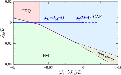
Figure 12: (Color online) Classical ground-state phase diagram of a dipolar spin ice described by $\mathcal{H_{\sf DSI}}$ [Eq. (7)], showing the breakdown of the chain picture of sufficiently strong, ferromagnetic third–neighbour interactions $J_{3d}$. The TDQ, CAF and FM states are composed of “chains” of ferromagnetically polarised spins. For $J_{3d}<-0.018D$, the FM and CAF phases are separated by a small region of non-chain states. Results are taken from a zero-temperature Monte-Carlo search of spin-ice configurations, for a cubic cluster of 128 sites. The parameters considered in soft–spin mean–field theory [Sec. III], classical Monte Carlo simulation [Sec. V], and quantum Monte Carlo simulation [Sec. VI], are indicated with a blue line.

For purpose of comparison with the mean–field theory of $\mathcal{H_{\sf DSI}}$ [Eq. (7)] developed in Sec III, and the numerical simulations described in Sec. V and Sec. VI, it is interesting to express the phase boundaries found from ${\mathcal{H}}^{\sf 2D}_{\sf Ising}$ [Eq. (46)] in terms of second–neighbour exchange $J_{2}$, setting all $J_{k\neq 2}\equiv 0$. Taking into account all $K_{\boldsymbol{\delta}}$ up to 7^th–nieghbour [cf. Table 2],we find that the transition between the CAF and TDQ occurs for

$$J_{2}/D=-0.0621\;,$$ (61)

while the transition between the TDQ and the FM occurs for

$$J_{2}/D=-0.0745\;.$$ (62)

These results are consistent with the results of classical Monte Carlo simulation, described in Sec. V, and in excellent agreement with the numerical values from zero–temperature quantum Monte Carlo simulation, described in Sec. VI, below. Mean field theory, on the other hand, is seen to over-estimate the stability of the TDQ phase, giving values of $J_{2}/D=-0.57$ [Eq. (33)] and $J_{2}/D=-0.80$ [Eq. (39)].

In the light of the recent experiments by Pomaranski et al. [pomaranski13, ], it is also interesting to ask what interchain couplings might arise in the spin–ice Dy₂Ti₂O₇. Taking values for exchange and dipolar interactions from Yavorskii et al. [yavorskii08, ], we find

$$K_{(1,\sqrt{2})}/D = -0.025\,,$$

$$K_{(2,0)}/D = \phantom{-}0.020\,,\qquad[\text{Dy${}_{2}$Ti${}_{2}$O${}_{7}$}]$$ (63)

$$K_{(0,2\sqrt{2})}/D = \phantom{-}0.001\,.$$

These parameters suggest that the classical ground state of Dy₂Ti₂O₇ would be a CAF — cf. Fig. 11. We return to this point in Section VII, below.

IV.3 Breakdown of the of chain–state picture

“Chain states”’ provide an extremely efficient way of minimising dipolar interactions ${\mathcal{H}}_{\sf dipolar}$ [Eq. (8)], but do not necessarily minimise the exchange interactions ${\mathcal{H}}_{\sf exchange}$ [Eq. (11)]. Given this, it is natural to ask how strong competing exchange interactions need to be to invalidate the “chain picture”. This proves to be a somewhat subtle question.

Exchange interactions up to third neighbour (cf. Fig. 3) can be grouped in three classes. First–neighbour interactions $J_{1}$ help determine the stability of the spin–ice manifold, but play no role in selecting an ordered ground state. Second–neighbour interactions $J_{2}$ can be combined with third–neighbour interactions $J_{3c}$ [see Appendix B], to give a combined interaction $J_{2}+3J_{3c}$. This combined interaction selects between different chain states, and does not by itself lead to any breakdown of the chain picture. Third–neighbour interactions $J_{3d}$ also selects between different chain states, but can also lead to a breakdown of the chain picture if ferromagnetic, and sufficiently strong.

To asses the impact of $J_{3d}$, we performed a numerical search for ground states of cubic clusters of 128, 432 and 1024 sites, using a zero-temperature Monte Carlo “worm” algorithm. Results for an 128-site cluster are shown in Fig. 12. Apart from a small window of parameters for $J_{3d}<0$, the ground state is dominated by the chain-based TDQ, CAF and FM states discussed above. The precise range of parameters for which non-chain states occur was found to depend on the geometry of the cluster. We note that no non-chain states were found for $J_{3d}>-0.018D$, in any cluster.

V Classical Monte Carlo simulation

The classical ground–states of dipolar spin ice are based on alternating chains of spins [Sec. III], a fact which can be understood through the mapping onto an effective Ising model [Sec. IV]. However, at finite temperature, a spin–ice can gain an extensive “ice entropy” by fluctuating between different spin–ice configurations. harris97 ; ramirez99 As a result, chain–based ordered ground states will give way to a classical spin liquid (CSL).

To learn more about the nature of this transition, and whether thermal fluctuations stabilise new ordered states, we have performed classical Monte Carlo simulations of $\mathcal{H_{\sf DSI}}$ [Eq. (12)]. Simulations were carried out for cubic clusters of 128 and 1024 spins, using the worm algorithm and parallel–tempering methods described in Appendix C, for 2${}^{\text{nd}}$–neighbour interaction $J_{2}/D$ spanning the cubic antiferromagnet (CAF), tetragonal double-Q (TDQ) and ferromagnetic (FM) ground states [cf. Fig. 11]. All other exchange interactions $J_{k\neq 2}$ were set to zero. The results of these simulations are summarised in Fig. 13.

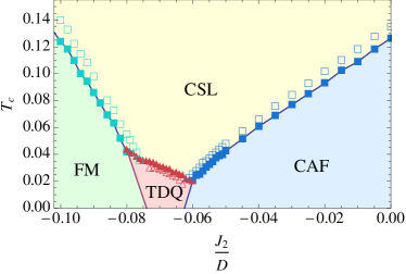
Figure 13: (Color online) Finite-temperature phase diagram of spin ice with long-range dipolar interactions, as a function of competing 2${}^{\text{nd}}$-neighbour exchange $J_{2}/D$. Results are taken from classical Monte Carlo simulation of $\mathcal{H}_{\sf DSI}$ [Eq. (7)] for cubic clusters of 128 (filled symbols) and 1024 spins (open symbols). The error in the estimate of $T_{c}$ is set by the interval between consecutive temperatures in simulations using parallel tempering.

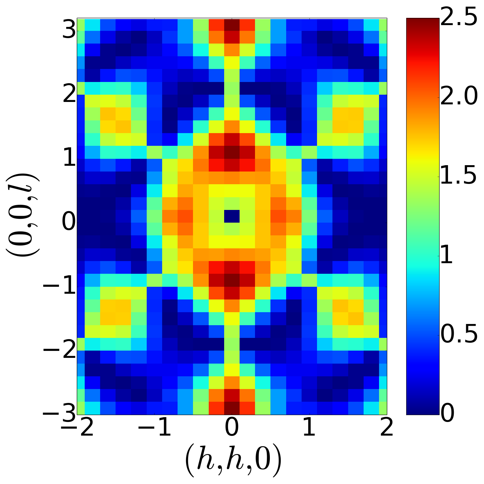
(a) $J_{2}/D=0.000$

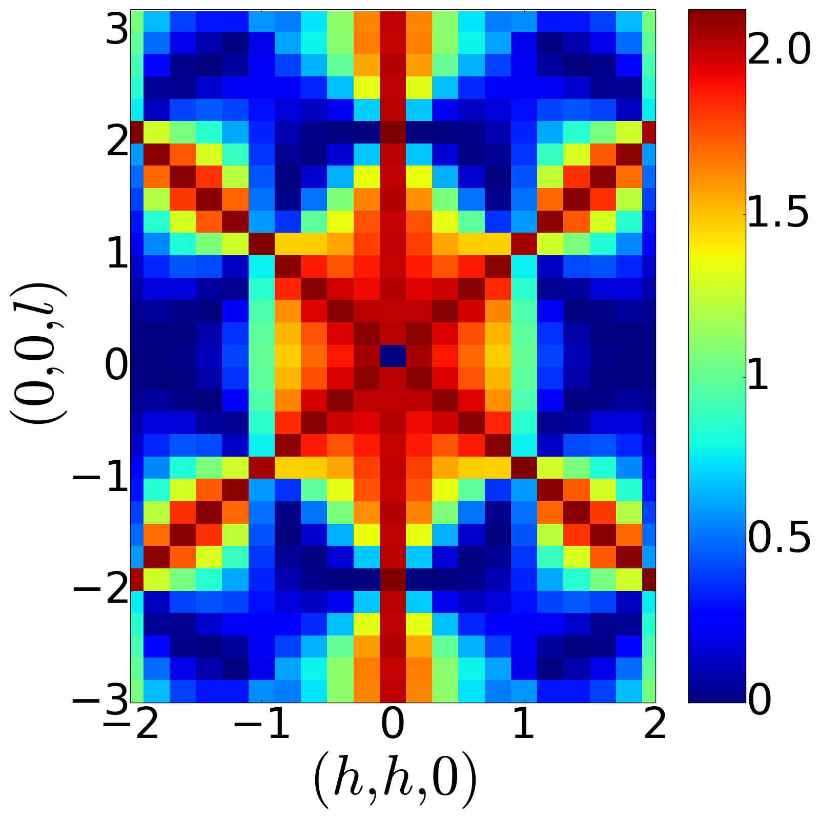
(b) $J_{2}/D=-0.070$

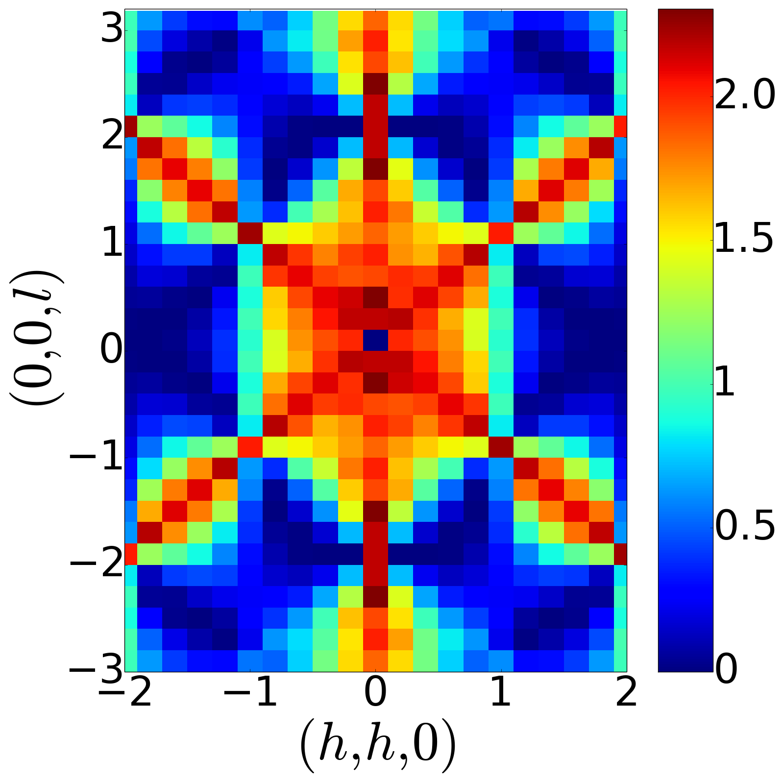
(c) $J_{2}/D=-0.090$

Figure 14: (Color online) Equal-time structure factor $S^{\sf SF}(\mathbf{q})$ [Eq. (66)] for a dipolar spin ice with competing further-neighbour exchange $J_{2}$, as found from classical Monte Carlo simulation of $\mathcal{H_{\sf DSI}}$ [Eq. (7)]. (a) $S^{\sf SF}({\bf q})$ for $J_{2}=0$. (b) $S^{\sf SF}({\bf q})$ for $J_{2}=-0.07D$. (c) $S^{\sf SF}({\bf q})$ for $J_{2}=-0.09D$. Simulations were performed for a cubic cluster of $2000$ spins, for parameters spanning the CAF, TDQ and FM ground states, for a temperature $T=0.5D$ within the disordered spin-ice regime, with $J_{k\neq 2}\equiv 0$. $S^{\sf SF}(\mathbf{q})$ is shown in the $[hhl]$ plane, in the spin-flip channel measured by Fennell et al. [fennell09, ].

V.1 Classical spin liquid

The finite–temperature phase diagram of dipolar spin ice is dominated by a classical spin liquid (CSL), shown in yellow in Fig. 13. This CSL has the character of a classical Coulombic phase, described by a $U(1)$ lattice gauge theory. henley10 For $J_{2}/D=0$, simulations reproduce known results for a purely dipolar spin ice, melko01 with the transition into the spin liquid occuring for $T_{c}/D\approx 0.12$. For ferromagnetic $J_{2}$, this transition temperature is at first suppressed, reaching a minimum value of $T_{c}/D\approx 0.02$ for $J_{2}/D\approx-0.06$. For stronger ferromagnetic $J_{2}$, there is a rise in $T_{c}/D$. These are the same trends as are observed in the overall band-width of spin-ice states [Fig. 5], within the mean–field theory described in Sec. III.

Spin correlations within the CSL phase are dipolar,isakov04 ; henley05 leading to singular “pinch–points”

$$S(\mathbf{q})\sim\left[\delta_{\alpha\beta}-\frac{q^{\alpha}q^{\beta}}{q^{2}}\right]$$ (64)

in the spin structure factor. Pinch–points of exactly this form have been observed in neutron scattering experiments on the spin ice Ho₂Ti₂O₇ by Fennell et al. [fennell09, ].

To characterise the CSL found in the presence of competing exchange interactions, we have used classical Monte Carlo simulation to calculate the (equal–time) structure factor

$$S^{\alpha\beta}(\mathbf{q})=\sum_{i,j=1}^{4}\langle S^{\alpha}_{i}(-{\bf q})S^{\beta}_{j}({\bf q})\rangle\;,$$ (65)

where $i,j$ run over the sites of a tetrahedron and the spin $S^{\alpha}_{i}$ is considered in frame of the cubic crystal axes $\alpha=\{x,y,z\}$. We consider in particular the spin–flip component of scattering, for neutrons polarised $\parallel[1\bar{1}0]$, as measured by Fennell et al. [fennell09, ] :

$$S^{\sf SF}(\mathbf{q}) = \sum_{i,j=1}^{4}\langle\left[{\bf S}_{i}(-{\bf q})\cdot{\bf u}({\bf q})\right]\left[{\bf S}_{j}({\bf q})\cdot{\bf u}({\bf q})\right]\rangle\;,$$ (66)

$${\bf u}({\bf q})=\hat{\bf n}\times{\bf q},\quad\hat{\bf n}=(1,\bar{1},0)/\sqrt{2}\;.$$

Simulation results for $S^{\sf SF}(\mathbf{q})$ in the CSL phase are shown in Fig. 14, for $\mathbf{q}$ in the $[hhl]$ plane, and a range of values of $J_{2}/D$ spanning the three classical ordered ground states. For $J_{2}/D=0$, these simulations reproduce known results for dipolar spin ice, with pinch–points clearly visible at a subset of reciprocal lattice vectors, e.g. $\mathbf{q}=(1,1,2)$ [cf. Fig. 14(a)]. For ferromagnetic $J_{2}/D<0$, there is a progressive redistribution of spectral weight within the $[hhl]$ plane [cf. Fig. 14(b, c)], None the less, pinch–points remain clearly defined.

V.2 Ordered phases

At low temperatures, in the absence of quantum tunnelling, long–range dipolar interactions drive dipolar spin ice into a state with chain–based order. Classical Monte Carlo simulation of $\mathcal{H_{\sf DSI}}$ [Eq. (12)] reveals the same three, chain–based ordered phases as are found in mean–field theory [Sec. III], and through mapping onto an effective Ising model [Sec. IV] : a cubic antiferromagnet (CAF), a tetragonal double-Q (TDQ) state and a cubic ferromagnetic (FM) [cf. Fig. 2]. Transition temperatures for the transition from the classical spin liquid (CSL) into each of these ordered states can be extracted from the susceptibility associated with the appropriate order parameter [cf. Eq. (38)].

The results of this analysis, for clusters of 128 and 1024 spins, are summarised in the finite–temperature phase diagram, Fig. 11, where the error on the estimated ordering temperature $T_{c}$ is indicated by the size of the point. All phase transitions are found to be first–order, with finite-size corrections to $T_{c}$ of order $10\%$ between the 128-site cluster and the 1024-site cluster. Classical Monte Carlo simulations do not reveal any new phases on the (degenerate) phase boundaries between the CAF and the TDQ, or the TDQ and the FM .

VI Quantum Monte Carlo simulation

Just as thermal fluctuations stabilize a classical spin liquid (CSL), so quantum tunneling might be expected to stabilize a quantum spin liquid (QSL), of the type previously studied in idealised models of a quantum spin-ice with nearest-neighbour interactions.hermele04 ; banerjee08 ; savary12 ; shannon12 ; benton12 ; lee12 ; savary13 ; gingras14 There is also the possibility that quantum fluctuations might stabilise new ordered states, not found in classical dipolar spin ice. To address these questions, we have carried out extensive quantum Monte Carlo (QMC) simulations of $\mathcal{H_{\sf QDSI}}$ [12].

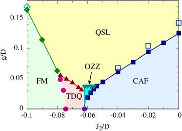
Figure 15: (Color online) Quantum ground-state phase diagram of a dipolar spin ice, as a function of competing 2^nd-neighbour exchange $J_{2}/D$, and quantum tunneling $g/D$. Results are taken from Green’s function Monte Carlo (GFMC) simulation of $\mathcal{H}_{\sf QDSI}$ [Eq. (12)], for cubic clusters of 128 sites (solid symbols) and 1024 spins (open symbols), with $J_{k\neq 2}=0$. Phase boundaries for $g/D=0$ were determined from the solution of the extended Ising model described in Sec. IV. Dashed lines bordering the OZZ state are taken from the degenerate perturbation theory described in Appendix E.

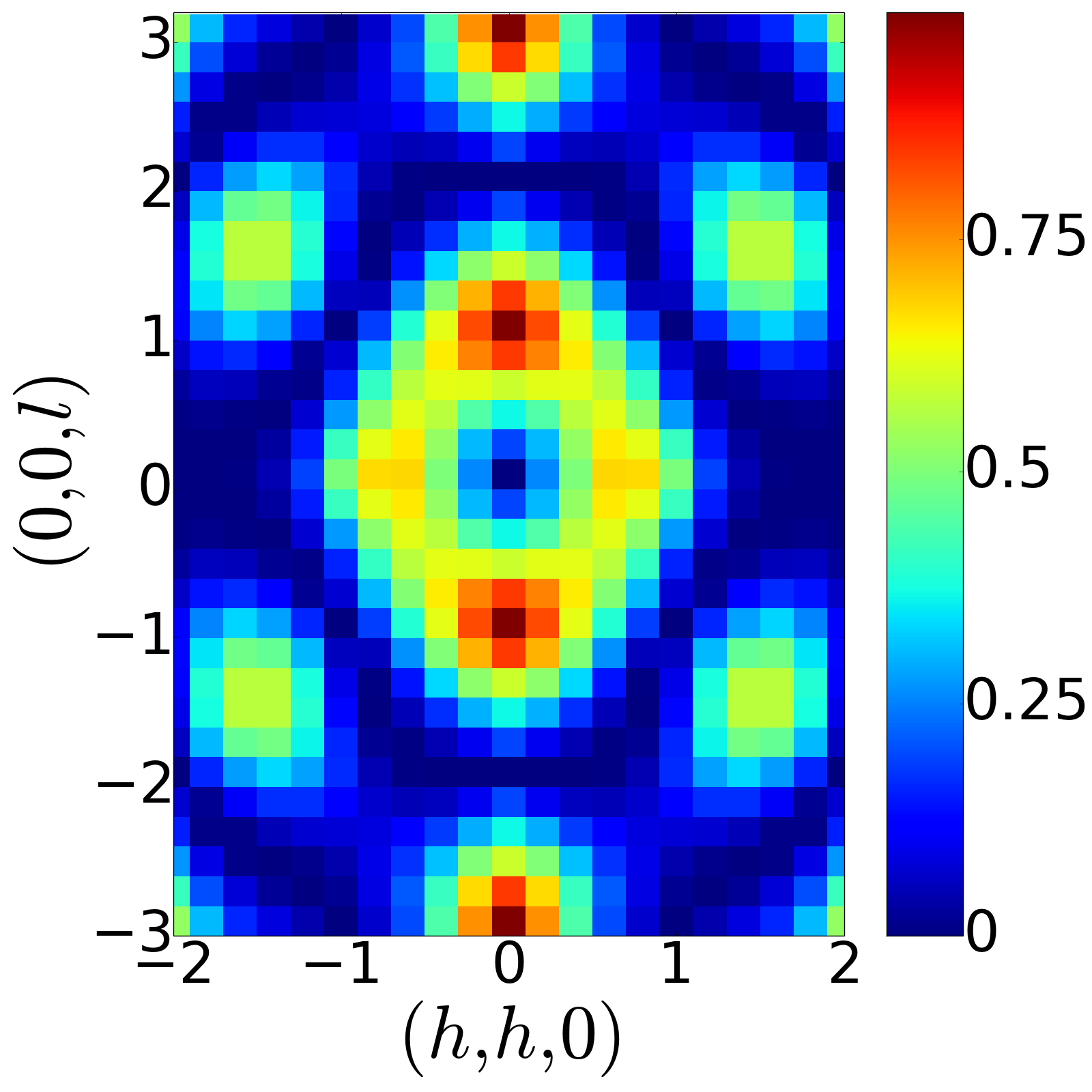
(a) $J_{2}/D=0.00$

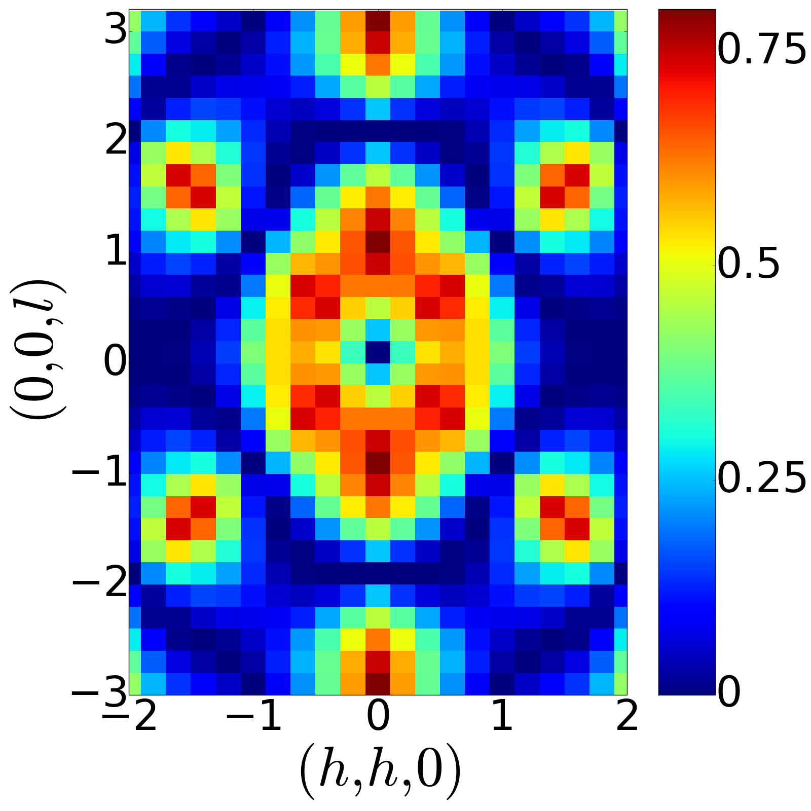
(b) $J_{2}/D=-0.07$

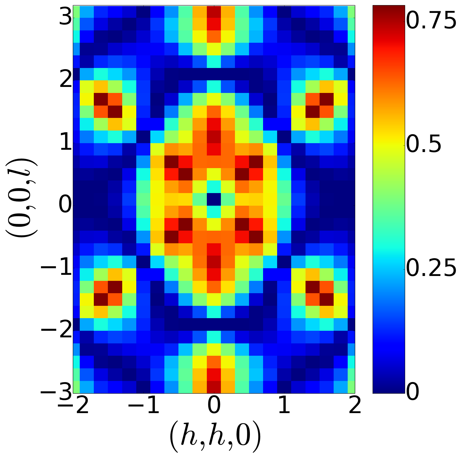
(c) $J_{2}/D=-0.09$

Figure 16: Equal-time structure factor $S^{\sf SF}(\mathbf{q})$ [Eq. (66)] for a dipolar spin ice with competing further-neighbour exchange $J_{2}$, as found from Green’s function Monte Carlo (GFMC) simulation of $\mathcal{H}_{\sf QDSI}$ [Eq. (12)]. (a) $S^{\sf SF}({\bf q})$ for $J_{2}=0$; (b) $S^{\sf SF}({\bf q})$ for $J_{2}=-0.07D$; and (c)$S^{\sf SF}({\bf q})$ for $J_{2}=-0.09D$. The sharp pinch–point structure, characteristic of classical spin ice, and visible in classical Monte Carlo simulations [cf. Fig. 14(a)–(c) at, e.g. ${\bf Q}=(1,1,1)$], is eliminated by quantum fluctuations. shannon12 ; benton12 All simulations were carried out for a cubic cluster of 2000 sites, with quantum tunnelling $g=0.5D$, and $J_{k\neq 2}\equiv 0$. $S^{\sf SF}({\bf q})$ is shown in the $[hhl]$ plane, in the spin-flip channel measured by Fennell et al. [Ref. fennell09, ].

Simulations of cubic clusters of 128 and 1024 spins were performed using the zero-temperature Green’s function Monte Carlo (GFMC) method described in Refs. [shannon12, ; benton12, ; sikora09, ; sikora11, ] and Appendix D. Within this approach, only spin–configurations satisfying the ice–rules are considered, and $\mathcal{H}_{\sf QDSI}$ [Eq. (12)] is taken to act on the space of all possible spin-ice ground states. GFMC simulations were carried out for a range of values of quantum tunnelling $g/D$, for 2${}^{\text{nd}}$–neighbour interaction $J_{2}/D$ spanning all three classical ground states [cf. Fig. 11]. All other exchange interactions $J_{k\neq 2}$ were set to zero. The results of these simulations are summarised in Fig. 15.

VI.1 Quantum spin liquid

The zero–temperature quantum phase diagram is dominated by a QSL phase, shown in yellow in Fig. 15. The minimum value of quantum tunneling $g_{c}$ needed to stabilize a QSL for a given value of $J_{2}/D$, closely tracks the transition temperature $T_{c}$ for $g=0$ [cf. Fig. 1]. Crucially, $g_{c}$ is always very small, being of order $g_{c}\sim 0.1D$ for $J_{2}/D=0$, and decreasing to a few percent of $D$ for $J_{2}/D\sim-0.06$.

Correlations within the QSL can once again be characterised by the equal–time structure factor $S(\bf q)$ [Eq. (65)]. While spin correlations in the CSL are dipolar leading to “pinch–points” in $S({\mathbf{q}})$ [cf. Fig. 14], spin correlations in the QSL decay as $1/r^{4}$ [hermele04, ], eliminating the pinch-points. shannon12 ; benton12 .

Results for $S^{\sf SF}({\mathbf{q}})$ [Eq. (66)], calculated using GFMC simulation, are shown in Fig. 16, for a range of values of $J_{2}/D$ spanning the phase diagram Fig. 15, and $g=0.5\ D>g_{c}$ within the QSL phase. As anticipated, the sharp zone–center pinch-points of the CSL are eliminated by quantum fluctuations [cf. Fig. 14]. Correlations are also suppressed near to ${\mathbf{q}}=0$ [cf. Ref. shannon12, ; benton12, ]. All of these features are universal characteristics of the QSL, and therefore independent of the values of $J_{2}$ and $D$.

Correlations at short wave length, on the other hand, show a marked imprint of the long–range dipolar interactions, when compared with results for $D=0$ [Ref. shannon12, ; benton12, ]. These features are only weakly constrained by the structure of the QSL, and therefore depend strongly on the ratio of $J_{2}/D$ for which the simulations were carried out.

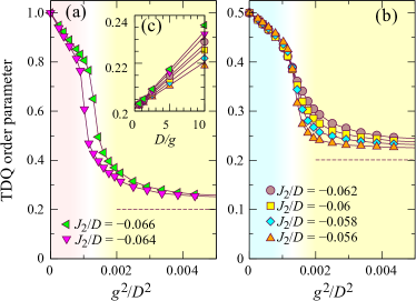
Figure 17: (Color online) Evidence for the transition from the quantum spin liquid (QSL) into ordered tetragonal double–Q (TDQ) and orthorhombic zig-zag (OZZ) ground states, as determined by Green’s function Monte Carlo (GFMC) simulation of $\mathcal{H}_{\sf QDSI}$ [Eq. (12)]. (a) Results for the order parameter ${\mathcal{O}}_{\sf TDQ}$ [Eq. (67)], showing the transition between the Quantum spin liquid (QSL) and TDQ phases. (b) Equivalent results for the transition between the QSL and OZZ phases. (c) [Inset to (a)] Scaling of order parameter within the QSL, showing how, for $D/g\to 0$, ${\mathcal{O}}_{\sf TDQ}\to 0.20(1)$, a finite-size value characteristic of the cluster simulated. Dashed lines in (a) and (c) show the corresponding asymptote for $g/D\to\infty$. Simulations were carried out for a cubic cluster of 128 sites, with $J_{k\neq 2}=0$. Values of $J_{2}/D$ are shown on the legend within the figure.

VI.2 Ordered ground states

For $g<g_{c}$, quantum fluctuations are not sufficient to stabilise a QSL, and the system orders. For $g\to 0$ we find the same three, chain–based states discussed in Sec. III and Sec. IV — a cubic antiferromagnet (CAF), a tetragonal double-Q (TDQ) state and a ferromagnet (FM). However quantum simulations also reveal a new ordered state, the orthorhombic zig–zag (OZZ) state shown in Fig. 2(d). The OZZ occurs at the boundary between the CAF and the TDQ, and is stabilised by quantum fluctuations at finite $g$. We consider each of these ordered states in turn, below.

The FM and CAF are “isolated states”, unconnected to other spin-ice configurations by matrix elements of $\mathcal{H}_{\sf tunneling}$ [Eq. (13)]. Quantum phase transitions between the QSL and the FM and CAF are therefore first-order, and can be determined by a simple comparison of ground state energies. The corresponding values of $g_{c}$, as a function of $J_{2}$, are shown in Fig. 15, for clusters of 128 and 1024 spins. Finite-size effects are relatively small, at least in the range of $J_{2}$ for which is was possible to converge simulations for both clusters.

The TDQ state, in contrast, is directly connected with QSL by matrix elements of $\mathcal{H}_{\sf tunneling}$. In this case $g_{c}$ was determined from a jump in the the order parameter of the TDQ state

$${\mathcal{O}}_{\sf TDQ}=\sum_{\eta=1}^{48}\sum_{j}\left\langle\left({\sf S}^{z,\text{\sf TDQ},\eta}_{j}\sf{S}^{z}_{j}\right)^{2}\right\rangle_{\text{\sf QMC}}$$ (67)

where the spin configurations ${\sf S}^{z,\text{TDQ},\eta}_{j}$ are drawn from the 48 different TDQ ground states enumerated in Table 1.

Results for ${\mathcal{O}}_{\sf TDQ}$ within GFMC simulation are shown in Fig. 17(a), for parameters spanning the TDQ and QSL states. An abrupt change in the order parameter marks the onset of TDQ order, with ${\mathcal{O}}_{\sf TDQ}\to 1$ in the fully ordered state. In the spin liquid, for $g>g_{c}$, ${\mathcal{O}}_{\sf TDQ}\to 0.20$, a finite-size value determined by the cluster used in simulations [cf. Fig. 17(b)].

The OZZ is one of the many degenerate classical ground states found at the border between the CAF and TDQ phases [cf. Sec. IV.2]. Unlike the CAF, the TDQ and OZZ both contain “flippable” hexagonal plaquettes where $\mathcal{H}_{\sf tunneling}$ [Eq. (13)] can act. As a result, both states gain energy from quantum fluctuations,

Besides having flippable plaquettes, the OZZ is also directly connected with the QSL. And, since the spin configurations in the one of the sets of parallel chains which make up the OZZ are identical to those of the TDQ (cf. Table. 1), it is also possible to use ${\mathcal{O}}_{\sf TDQ}$ [Eq. (67)] as an order parameter for the OZZ state. Corresponding results for ${\mathcal{O}}_{\sf TDQ}$ are shown in Fig. 17(b), for parameters spanning the OZZ and QSL states. We note that, in this case, ${\mathcal{O}}_{\sf TDQ}\to 0.5$ in the fully ordered state.

Colllecting all of these results, we obtain the quantum ground state phase shown in Fig. 15. We find that a small fan of OZZ order opens from the highly degenerate point $J_{2}/D=-0.0621$, $g/D=0$, at the expense of the CAF. Detail of this highly frustrated region of the phase diagram is given in Fig. 18.

It is possible to estimate the phase boundaries between the TDQ, OZZ and CAF states from 2${}^{\text{nd}}$–order perturbation theory in $g$, as described in Appendix E. The corresponding results are shown as dashed lines in Fig. 15 and Fig. 18. In the case of the boundary between the CAF and OZZ states, it is possible to make direct comparison between this perturbation theory and GFMC. As shown in Fig. 15, the agreement is excellent.

While no new ordered states, besides the OZZ, were found for GFMC simulations of cubic clusters of 128 or 1024 states, it is interesting to speculate that quantum fluctuations might stabilise further new ordered state in the thermodynamic limit — perhaps in the form of the “fans” found in classical anisotropic next-nearest neighbour Ising (ANNNI) models. bak82 ; selke88 It is also plausible that thermal fluctuations might stabilise the OZZ, or some other state like it, in a more general model.

VII Application to spin–ice materials

In this Article we have used a variety of numerical and analytic techniques to explore the nature of the equilibrium ground state of a dipolar spin ice with competing exchange interactions and quantum tunnelling between different spin–ice configurations, as described by $\mathcal{H_{\sf QDSI}}$ [Eq. (12)].

A clear picture emerges from this analysis. Long–range dipolar interactions, ${\mathcal{H}}_{\sf dipolar}$ [Eq. (8)], are minimised by states composed of ferromagnetically polarised chains of spins, within which they are exponentially screened. Exchange interactions, ${\mathcal{H}}_{\sf exchange}$ [Eq. (11)] act to select between such “chain states”, and in the absence of quantum fluctuations the ground state of a dipolar spin ice is one of the three ordered states, described in Table 1. Quantum tunnelling between different spin–ice configurations, $\mathcal{H}_{\sf tunneling}$ [Eq. (13)], can stabilise new forms of chain–based order, and if sufficiently strong, will drive a quantum spin liquid ground state. We now consider the implication of these results for real materials, paying particular attention to the dipolar spin ice, Dy₂Ti₂O₇.

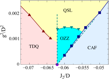
Figure 18: (Color online) Detail of the ground-state phase diagram of a dipolar spin ice [Fig. 15], showing how a small fan of orthorhombic zig-zag (OZZ) order opens between the cubic antiferromagnet (CAF) and tetragonal double–Q (TDQ) states. Filled symbols show the results of Green’s function Monte Carlo (GFMC) simulation of $\mathcal{H}_{\sf QDSI}$ [Eq. (12)], as described in the text. Dashed lines show the predictions of the degenerate perturbation theory described in Appendix E. Simulations were carried out for a cubic cluster of 128 sites, with $J_{k\neq 2}=0$.

Dy₂Ti₂O₇ is perhaps the best studied of spin–ice materials. Pioneering measurements of the heat capacity of Dy₂Ti₂O₇ by Ramirez et al. [ramirez99, ] provided the first thermodynamic evidence for the existence of an extensive ground–state degeneracy, as predicted by the “ice rules” [pauling35, ]. These results are consistent with subsequent measurements of the heat–capacity of Dy₂Ti₂O₇ by other groups. higashinaka02 ; hiroi03 ; klemke11 And, significantly, none of these studies reported evidence for a transition into an ordered ground state at low temperatures, despite the expectation that a classical dipolar spin ice should have an ordered ground state. melko01

As the understanding of spin ice has improved, it has become clear that non–equilibrium effects play an important role, and that the thermodynamic properties of materials like Dy₂Ti₂O₇ are consequently subject to extremely long equilibriation times. castelnovo12 In the light of this, the evolution of the low–temperature heat capacity of Dy₂Ti₂O₇ was recently revisted by Pomaranski et al. [pomaranski13, ], using an experimental setup designed to track the equilibration of the sample. Their study reports equilibration times in excess of 4 days at $340\ \text{mK}$, and a dramatically revised profile for the low–temperature specific heat. pomaranski13 One of the most striking features of these results is an upturn in $\partial S/\partial T|_{V}=C_{V}/T$ below $T\approx 500\text{mK}$, suggestive of an ordering transition, of the type studied in Sec. V, or the emergence of a new (quantum) energy scale.

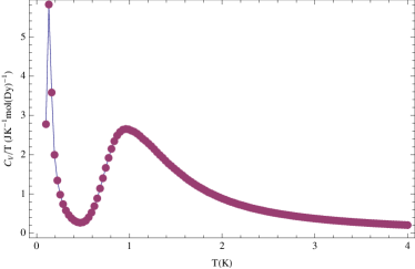
Figure 19: (Color online) Plot of heat capacity $C_{\rm V}$ divided by temperature, $T$, for a dipolar spin ice described by $\mathcal{H_{\sf DSI}}$ [Eq. (7)], with parameters taken from fits to experiment on Dy₂Ti₂O₇ [yavorskii08, ], as specified in [Eq. (II.3)]. Results are taken from classical Monte Carlo simulation of a cluster of $128$ spins.

The results of Pomoranskii et al. [pomaranski13, ] clearly motivate a number of questions, including : What is the origin of the upturn in $C_{V}/T$ ? What is the nature of the ground state of Dy₂Ti₂O₇ ? And, what is the reason for its extremely slow approach to equilibrium ?

These questions are most easily addressed within the well–established, classical, dipolar spin–ice model $\mathcal{H_{\sf DSI}}$ [Eq. (7)]. As discussed in Sec. IV.2, the parameters reported by Yavorskii et al. [yavorskii08, ], place the classical ground state of Dy₂Ti₂O₇ in the cubic antiferromagnetic (CAF) phase [cf. Fig. 2(a)], previously investigated by Melko et al. [melko01, ]. It is therefore natural to ask whether the upturn in $C_{V}/T$, observed in Dy₂Ti₂O₇ [pomaranski13, ], marks the onset of CAF order ?

At present, it is only possible to approach this question with reference to the heat capacity measurements of Pomaranskii et al. [pomaranski13, ]. To this end, in Fig. 19 we show estimates of $C_{V}/T$ taken from classical Monte Carlo simulations of $\mathcal{H_{\sf DSI}}$ [Eq. (7)], for the parameters given by Yavorskii et al. [yavorskii08, ] — cf. Eq. (II.3). Simulations were carried out using the methods described in Appendix C, for a cubic cluster of 128 sites. A complete comparison between experiment and simulation is not possible, since experimental data for $C_{V}/T$ is only available down to $T=340\ \text{mK}$ [pomaranski13, ]. However simulations correctly reproduce the measured peak in $C_{V}/T$ at $T\approx 1\ \text{K}$, characteristic of the onset of spin-ice correlations, and exhibit a second peak at $T\approx 100\ \text{mK}$, associated with a first-order transition into the CAF ground state. For temperatures $340<T\lessapprox 500\ \text{mK}$, simulations suggest an upturn in $C_{V}/T$ which is reminiscent of, but a little weaker than, that observed in experiment.

At first sight, the comparison between simulation might seem good enough to justify a diagnosis of CAF order. However the CAF is only one of the infinite family of chain–based ground states described by the effective Ising model ${\mathcal{H}}^{\sf 2D}_{\sf Ising}$ [Eq. (46)] — cf. Sec. IV. And, since dipolar interactions are exponentially screened within these chain–states — cf. Sec. IV.1 — the nature of the classical ground state is extremely sensitive to small differences in the exchange interactions ${\mathcal{H}}_{\sf exchange}$ [Eq. (11)].

For the specific set of parameters provided by Yavorskii et al. [yavorskii08, ] — Eq. (II.3) — the inter–chain interactions of ${\mathcal{H}}^{\sf 2D}_{\sf Ising}$ [Eq. (46)] take on the values

$$K_{(1,\sqrt{2})} = -35\;\text{mK}\,,$$

$$K_{(2,0)} = \phantom{-}28\;\text{mK}\,,\qquad[\text{Dy${}_{2}$Ti${}_{2}$O${}_{7}$}]$$ (68)

$$K_{(0,2\sqrt{2})} = \phantom{-}1\;\text{mK}\,.$$

These very weak interactions between chains should be compared with the uncertainty in exchange interactions, which is at least $10\ \text{mK}$ [yavorskii08, ].

It follows from definition of $K_{\boldsymbol{\delta}}$ [cf. Table 2], that any change $\delta J_{k}$ in the value of exchange parameters leads directly to a change $\delta K_{\boldsymbol{\delta}}$ in the interactions between chains of spins

$$\delta K_{(1,\sqrt{2})} = -\delta J_{2}/3-\delta J_{3c}-\delta J_{3d}\,,$$

$$\delta K_{(2,0)} = \delta J_{3d}\,.$$ (69)

Since the parameters given by Yavorskii et al. [yavorskii08, ] place Dy₂Ti₂O₇ close to borders of CAF, tetragonal double Q (TDQ) and ferromagnetic (FM) phases — cf. Fig. 11 — an error as small as $\delta J\sim 7\,\text{mK}$ could be enough to convert the CAF into a TDQ ground state, while $\delta J\sim 50\,\text{mK}$ could stabilize a FM.

This extreme sensitivity of the ground state of dipolar spin ice to small changes in exchange interactions makes very challenging to reliably predict the ground state in a real material from high-temperature estimates of model parameters. However this challenge brings with it an opportunity : it seems entirely plausible that changes in $J_{k}$ of the scale $\delta J\sim 50\,\text{mK}$ could be achieved through the application hydrostatic pressure, or by chemical substitution,zhou12 allowing a spin ice to be tuned from one ground state to another.

The “chain picture” of ground–state order in a dipolar spin ice may also offer some insight into the very slow equilibration of Dy₂Ti₂O₇ at low temperatures. pomaranski13 In order to achieve an ordered, equilibrium ground state, a dipolar spin ice must first select the low–energy chain–based states from the extensive set of states obeying the ice rules, and then single out the chain–state with the lowest energy. At low temperatures, this thermal equilibration will be achieved through the motion of magnetic monopoles. However, to connect one chain–state with another, a monopole would have to reverse all of the spins in chain. This can only be achieved by the monopole traversing the entire length of a chain — potentially the entire width of the sample. Such dynamics would be activated, since it costs energy to make a pair of monopoles, and extremely slow.

The range of possible outcomes for the low–temperature physics of Dy₂Ti₂O₇ becomes much richer once quantum effects are taken into account. One possibility is that quantum tunnelling, of the type described by ${\mathcal{H}}_{\sf tunneling}$ [13] could stabilise a quantum spin–liquid (QSL) ground state, described by a quantum $U(1)$ lattice gauge theory [cf. Sec. VI]. In this case, the upturn in $C_{V}/T$ would signal the crossover between the classical and a quantum spin liquid regimes. benton12 ; kato-arXiv

Another possibility, where exchange interactions place the system close to a classical phase boundary, is that quantum fluctuations could stabilise a new form of order, such as the orthorhombic zig–zag (OZZ) state studied in Sec. VI.2. Such a ground state could melt into a classical (or quantum) spin liquid at finite temperature, leading to an upturn in $C_{V}/T$.

No reliable estimate is currently available for the strength of quantum tunneling in Dy₂Ti₂O₇. And the uncertainty in published estimates of exchange interactions is also too great to assess how close it lies to a classical phase boundary. For both reasons, it is difficult to draw any firm conclusions about the quantum or classical nature of its ground state. iwahara15 ; rau-arXiv ; tomasello-arXiv

However, one of the interesting consequences of chain–based order, and in particular of the exponential screening of dipolar interactions within chain states, is that quantum tunnelling does not need to be very strong to have a significant effect. From Quantum Monte Carlo simulations for parameters similar to those proposed for Dy₂Ti₂O₇ [cf. Sec. VI.1], we estimate that the value of quantum tunnelling $g$ needed to stabilize a QSL may be as little as $g^{\text{Dy${}_{2}$Ti${}_{2}$O${}_{7}$}}_{c}\approx\;70\;\text{mK}$.

Consequently — and perhaps counter–intuitively — a “classical” spin ice like Dy₂Ti₂O₇, in equilibrium, may not be bad place to look for a QSL. In this context it is interesting to note that the pinch–points observed in Dy₂Ti₂O₇, morris09 and its sister compound Ho₂Ti₂O₇, fennell09 are somewhat reminiscent of the QSL at finite temperature. benton12 ; kato-arXiv

VIII Conclusions

In conclusion, determining the zero-temperature, quantum, ground state of a realistic model of a spin ice is an important challenge, motivated by recent experiments on Dy₂Ti₂O₇ pomaranski13 and ongoing studies of quantum spin-ice materials. thompson11 ; ross11-PRX1 ; chang12 ; fennell12 ; fennell14 ; kimura13 In this Article, we have used a variety of numerical and analytic techniques to address the question : “What determines the equilibrium ground state of spin ice, once quantum effects are taken into account ?”

In Sec. III and Sec. IV, we have shown how a new organisational principle emerges : ordered ground states in a dipolar spin ice are built of alternating chains of spins, with net ferromagnetic polarisation. These “chain states” minimise long–range dipolar interactions, and provide a natural explanation for the slow dynamics observed in Dy₂Ti₂O₇ [pomaranski13, ]. And, since dipolar interactions are exponentially screened within chain states, they can be described by an extended Ising model on an anisotropic triangular lattice, ${\mathcal{H}}^{\sf 2D}_{\sf Ising}$ [Eq. (46)].

In Sec. V and Sec. VI, using Monte Carlo simulation, we have determined both the quantum and classical phase diagrams of ${\mathcal{H}}_{\sf QDSI}$ [Eq. (12)], as a function of quantum tunneling $g$, and temperature $T$. We find that only a modest amount of quantum tunneling $g_{c}$ is needed to stabilize a quantum spin liquid (QSL), with deconfined fractional excitations, hermele04 ; banerjee08 ; savary12 ; shannon12 ; benton12 ; lee12 ; savary13 ; moessner03 . These results are summarized in Fig. 1.

We have also considered the implication of these results for real materials, concentrating on the spin ice Dy₂Ti₂O₇. Based on published estimates of exchange parameters,yavorskii08 we find that an ordered ground state in Dy₂Ti₂O₇ would be a cubic antiferromagnet (CAF). However this state lies tantalisingly close in parameter space to other, competing ordered phases, and only a very small amount of quantum tunneling would be needed to convert it into a quantum spin liquid.

While we have chosen to emphasize Dy₂Ti₂O₇, there are a great many rare-earth pyrochlore oxides,gardner10 in which to search for quantum spin ice, and other unusual forms of magnetism.savary12 ; lee12 ; yan-arXiv In many of these materials, dipolar interactions will also play a role, and the small values of $g_{c}$ found in our simulations offer hope that quantum spin-liquids may be found in other materials at low temperature.

Appendix A Ewald summation of long-range dipolar interactions

The quantum and classical Monte Carlo simulations described in this Communication were carried out for cubic clusters of $N=16\times L^{3}=128,\,432,\,1024,\,2000$ spins, with periodic boundary conditions. The long-range dipolar interactions ${\mathcal{H}}_{\sf dipolar}$ [Eq. (8)], which cross the periodic boundaries of the cluster, were treated by Ewald summation.

Imposing periodic boundary conditions on a cubic cluster of dimension $L$, converts it into an infinitely-extended system, repeating with period $L$, for which the sum over long-range dipolar interactions is only conditionally convergent. Within Ewald summation, this slowly converging sum, $U={\mathcal{H}}_{\sf dipolar}/D$, is divided into two rapidly and absolutely convergent sums, $U^{({\rm R})}$ — which is evaluated in real space, and $U^{({\rm G})}$ — which is evaluated in reciprocal space. The rate of convergence of both sums is determined by a parameter $\alpha$, with dimension of inverse length, which determines the crossover between short-range interactions (treated in real space) and long-range interactions (treated in reciprocal space). Since the system is periodic, the self-energy $U^{({\rm SE})}$ arising from a spin interacting with an infinite number of copies of itself must also be taken into account. And since it is infinitely-extended, care must also be taken to impose an appropriate boundary condition at infinity.

Following [wang01, ], we impose boundary conditions through a macroscopic field term $U^{({\rm MF})}$, and write

$${\mathcal{H}}_{\sf dipolar}/D=U^{({\rm R})}+U^{({\rm G})}+U^{({\rm SE})}+U^{({\rm MF})}\,.$$ (70)

The sum evaluated in real space is given by

$$U^{({\rm R})} = \frac{1}{2}\sum_{i,j=1}^{N}\sum_{{\bf n}}^{\prime}\left\{\left({\bf S}_{i}\cdot{\bf S}_{j}\right)F_{1}(|{\bf R}_{ij}+{\bf n}|)-\left[{\bf S}_{i}\cdot({\bf R}_{ij}+{\bf n})\right]\left[{\bf S}_{j}\cdot({\bf R}_{ij}+{\bf n})\right]F_{2}(|{\bf R}_{ij}+{\bf n}|)\right\}\;,$$ (71)

$$F_{1}(x) = \frac{1}{x^{3}}\left({\rm erfc}\left(\alpha x\right)+\frac{2\alpha x}{\sqrt{\pi}}e^{-\alpha^{2}x^{2}}\right)\;,$$ (72)

$$F_{2}(x) = \frac{1}{x^{5}}\left(3\,{\rm erfc}\left(\alpha x\right)+\frac{2\alpha x}{\sqrt{\pi}}\left(3+2\alpha^{2}x^{2}\right)e^{-\alpha^{2}x^{2}}\right)\;,$$ (73)

where ${\bf n}\equiv(n_{x},n_{y},n_{z})L$ with $n_{a}\in{\mathbb{Z}}$, and the prime on $\sum^{\prime}_{{\bf n}}$ indicates that the divergent terms arising for ${\bf n}=0$ and $\mathbf{R}_{ij}=0$ are omitted from the sum. The functions $F_{1}(x)$ and $F_{2}(x)$, which control the convergence of $U^{({\rm R})}$, are expressed in terms of the complementary error function ${\rm erfc}(z)$. The real space sum runs over all the periodic images of the cubic cluster of dipole moments.

The sum to be evaluated in reciprocal space is a sum over the points ${\bf G}\equiv(G_{x},G_{y},G_{z})L$ (with $G_{a}\in{\mathbb{Z}}$) of the reciprocal lattice:

$$U^{({\rm G})}=\frac{1}{2L^{3}}\sum_{\mathbf{G}\neq 0}\frac{4\pi}{G^{2}}\exp\left[-\left(\frac{\pi G}{\alpha L}\right)^{2}\right]\sum_{i,j=1}^{N}\left({\bf S}_{i}\cdot{\bf G}\right)\left({\bf S}_{j}\cdot{\bf G}\right)\exp\left(\frac{2\pi i}{L}{\bf G}\cdot{\bf R}_{ij}\right)\;.$$ (74)

The self-energy of spins is given by

$$U^{({\rm SE})}=-\frac{2\alpha^{3}}{3\sqrt{\pi}}\sum_{i=1}^{N}{\bf S}^{2}_{i}\,.$$ (75)

The boundary conditions “at infinity” are imposed by the macroscopic field term

$$U^{({\rm MF})}=\frac{2\pi}{\left(2\epsilon+1\right)L^{3}}\sum_{i=1}^{N}\sum_{j=1}^{N}{\bf S}_{i}\cdot{\bf S}_{j}\,,$$ (76)

where the choice of boundary conditions is determined by the effective “permitivity” $\epsilon$.

In this work we make the choice $\epsilon\rightarrow\infty$. This is equivalent to embedding the periodic array of finite-size clusters in a medium which perfectly screens the net dipole moment of each cluster, so that the macroscopic field term $U^{({\rm MF})}\to 0$. The main justification for this choice of boundary condition comes from the perfect quantitative agreement between the results of classical Monte Carlo simulation in the limit $T\to 0$, and the classical ground states determined through mapping onto an effective Ising model, as described in Section IV. In real materials, phases with a net moment, such as the ferromagnet (FM), will form domains to screen the macroscopic field, and the effective boundary condition “at infinity” will also depend on the shape of the sample.

Appendix B Equivalence of exchange interactions within the spin–ice manifold

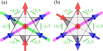
Figure 20: (Color online) Equivalence of the exchange interactions $J_{2}$ and $J_{3c}$ within the manifold of spin-ice configurations. All possible spin-ice states can be constructed from the two configurations (a) and (b), with energies $E_{a}$ [Eq. (79)] and $E_{b}$ [Eq. (80)]. In both cases, the energy is a function of $J_{2}+3J_{3c}$, and the effect of the two exchange interactions is equivalent, up to a factor $3$. Ferromagnetic chains of spins, which form the building-block for ordered states, are shown by thick magenta and green lines.

For spin–configurations obeying the “ice rules”, a further simplification arises from the fact that second–neighbour exchange $J_{2}$, and the third–neighbour exchange in the direction of the $[110]$ chains, $J_{3c}$, are no longer independent parameters.

To understand how this works, we consider the two corner–sharing tetrahedra shown in Fig. 20. The 2–in, 2–out “ice–rule” reduces the number of possible spin-configurations from $2^{7}=128$, to 18. Each of these 18 configurations is equivalent to one of the two configurations shown in Fig. 20. The energy of these spin configurations can be calculated by counting the number of satisfied and unsatisfied bonds of each type. Second–neighbour bonds (denoted by green lines) contribute

$$\delta E_{J_{2}}=\pm\ J_{2}/3\;.$$ (77)

Third–neighbour bonds, of the type $J_{3c}$, meanwhile, contribute

$$\delta E_{J_{3c}}=\pm J_{3c}\;.$$ (78)

Counting the relevant bonds, we find that the energies of the spin configurations shown in Fig. 20(a) and Fig. 20(b), are given by

$$E_{a}=\phantom{-}\frac{2}{3}J_{2}+3J_{3c} = J_{3c}+\frac{2}{3}\left(J_{2}+3J_{3c}\right)\;,$$ (79)

$$E_{b}=-\frac{2}{3}J_{2}-J_{3c} = J_{3c}-\frac{2}{3}\left(J_{2}+3J_{3c}\right)\;.$$ (80)

Comparing the two results, we see that the interactions $J_{2}$ and $J_{3c}$ both have the same effect — up to a factor $\times 3$ — when acting on any spin–configuration obeying the ice rules. The constant shift $J_{3c}$, which appears in both $E_{a}$ [Eq. (79)] and $E_{b}$ [Eq. (80)], is the same for all spin-ice configurations, and so does not distinguish between different ordered or disordered states.

The physically relevant parameter, within a spin–ice, is therefore

$$J_{2}+3J_{3c}\;,$$ (81)

as given in Section II.3.

Appendix C Classical Monte Carlo - technical details

Our classical Monte Carlo was carried out using cubic cells with periodic boundary conditions with $16\times L^{3}$ Ising spins with $L=2,3,4,5$, though for the phase diagram we chose cubic clusters with $128$ ($L=2$) and $1024$ ($L=4$), compatible with all three ordered phases. The long-ranged dipolar interaction was handled using a pre-tabulated Ewald summation (see Section A and Ref. [mcclarty14, ]). As is now standard for simulations of spin ice, the Monte Carlo allowed for single spin flips and worm updates.melko01 The worm updates allow for efficient sampling of spin-ice states with a short autocorrelation time compared to simulation time scales. We simulated up to $128$ temperatures simultaneously on the hydra cluster based in Garching with parallel tempering moves to assist equilibration. The highest temperature was taken below the heat capacity peak into the ice states. The simulations for $L=4$ at low temperature were somewhat hampered by slow equilibration despite the presence of loop moves and parallel tempering. Whereas $L=2$ simulations were found to be independent of the starting configuration, this ceased to be the case for $L=4$. We therefore conducted simulations by starting from each of the three known ordered states and also from states that are degenerate at the phase boundaries — for example the orthorhombic zigzag state (OZZ).

Appendix D Quantum Monte Carlo - technical details

We have performed Green’s function Monte Carlo (GFMC) simulations of $\mathcal{H}_{\sf QDSI}$ [12], using methods previously developed to study the quantum dimer model on a diamond lattice,sikora09 ; sikora11 and quantum spin ice in the absence of long-range dipolar interactions. shannon12 ; benton12 GFMC is a form of zero-temperature Quantum Monte Carlo simulation, which is numerically exact where simulations converge.

Our implementation of GFMC closely parallels that of [calandra-buonaura98, ]. We work explicitly with spin–ice configurations and, starting from a given spin configuration, use a population of “walkers” to sample the space of other configurations connected by off-diagonal matrix elements of the Hamiltonian, $\mathcal{H}_{\sf QDSI}$ [12]. A guide wave function, optimised by a separate variational Monte Carlo simulation is used to improve the convergence of simulations. As such, GFMC can be thought of as a systematic way of improving upon a variational wave function. A suitable variational wave function for a quantum spin ice, based on plaquette-plaquette correlations, is described in [sikora11, ]. The number of variational parameters used in simulations, depended on the cluster, and was typically 20-40. Populations of up to 1000 walkers were used in GFMC simulation. The population of walkers was reconfigured after a typical period of 45 steps, with simulations run for a few thousand consecutive reconfigurations. The averages used in estimators for the ground state energy, etc., were calculated for sequences of 50-300 steps.

We performed GFMC simulations for clusters of 128, 1024, and 2000 sites, with the full cubic symmetry of the pyrochlore lattice. Since not all of the ordered states considered are compatible with the 2000-site cluster, this was used to explore the correlations $S(\mathbf{q})$ of the QSL phase, and not to determine the ground-state phase diagram. To test the accuracy of the method, simulations of were also performed for a 80-site cluster with lower symmetry. Exact diagonalization calculations were carried out for the same 80-site cluster, and found to be in perfect numerical agreement with the results of GFMC.

Simulations for “large” values of $g\gtrsim 0.1D$, within the QSL, are relatively easy to converge, since all spin-ice configurations, apart for a tiny subset of “isolated states”, are connected by matrix elements of $\mathcal{H}_{\sf QDSI}$ [12], and all spin-ice configurations enter into the QSL ground state with comparable weight. Simulations are relatively difficult to converge for large clusters and “small” values of $g$, especially in the highly frustrated region $-0.08\lesssim J_{2}/D\lesssim-0.06$, where the coupling between parallel “chains” is vanishingly small and many different ground states compete. Detail of this region of the phase diagram is given in Fig. (18).

The Hilbert space of different possible spin–ice configurations, on which $\mathcal{H}_{\sf QDSI}$ [12] acts, can be divided into distinct topological sectors, according to the net flux of spin moments through the boundaries of a cluster shannon12 ; sikora11 . Under the dynamics described by $\mathcal{H}_{\sf QDSI}$, these fluxes are conserved. The QSL, and the CAF, TDQ and OZZ ground state all belong to the zero–flux sector, while the FM has a finite value of flux. We have GFMC performed simulations in a representative selection of flux sectors, and find no evidence of other competing ground states with finite values of flux. We have also verified that the energies of the QSL in different flux sectors satisfies the expected scaling with flux at fixed system size, as described in Ref. shannon12, .

Table 3: Ground state energy $E_{0}$, excitation gap $\Delta$ and number of flippable plaquettes $N_{\text{flip}}$ for cubic clusters with $N=128$ and $N=1024$ sites, used in constructing the degenerate perturbation theory Eq. (82).

state	$N$	$E_{0}/N$	$\Delta_{0}$	$N_{\text{flip}}$
CAF	128	$-1.94759D-2J_{2}/3$		$0$
CAF	1024	$-1.94760D-2J_{2}/3$		$0$
OZZ	128	$-1.92688D-J_{2}/3$	$0.2906D+8J_{2}/3$	32
OZZ	1024	$-1.92687D-J_{2}/3$	$0.2919D+8J_{2}/3$	256
TDQ	128	$-1.90617D$	$-0.3725D-8J_{2}$	32
TDQ	1024	$-1.90613D$	$-0.3717D-8J_{2}$	256

Appendix E 2${}^{\text{nd}}$ order perturbation theory in $g$

We can use perturbation theory in $g$ to calculate the effect of the quantum fluctuations about the TDQ and OZZ ground states. To second order in $g$, the ground state energy is given by

$$E^{(2)}=E^{(0)}-N_{\text{flip}}\frac{g^{2}}{\Delta_{0}}\,,$$ (82)

where $E^{(0)}$ is the classical ground state energy and $\Delta_{0}$ is the energy gap between the ground state and the excited state obtained by flipping the spins on a hexagon (where $N_{\text{flip}}$ is the number of such hexagons, and all the flippable hexagons are equivalent). These numbers, found by the numerical enumeration of states, are presented for the 128 and 1024 site cluster in Table 3.

Comparing these energies close to the classical phase boundary where the TDQ, the OZZ, and the CAF are degenerate, we get that OZZ state has the lowest energy and is stabilized between the TDQ and CAF phases. The phase transition lines between the TDQ and OZZ phases are essentially independent of $g$:

$$J_{2}/D =-0.0621\quad\text{(128 sites)}\,,$$ (83)

$$J_{2}/D =-0.0622\quad\text{(1024 sites)}\,.$$ (84)

In contrast, the phase boundaries between the CAF and OZZ depend on $g/D$ as

$$J_{2}/D =-0.0621+6.01(g/D)^{2}\quad\text{(128 sites)}\,,$$ (85)

$$J_{2}/D =-0.0622+5.95(g/D)^{2}\quad\text{(1024 sites)}\,.$$ (86)

These phase boundaries are shown in Fig. 15 and Fig. 18 as dashed lines (the finite–size effects are not discernible on the scale of the figure).

References

- (1) P. Fazekas and P. W. Anderson, Phil. Mag. 30, 423 (1974).
- (2) Patrick A. Lee Science 321, 1306 (2008).
- (3) Leon Balents, Nature, 464 199 (2010).
- (4) S. T. Bramwell and M. J. P. Gingras, Science 294, 1495 (2001).
- (5) C. Castelnovo, R. Moessner, and S. L. Sondhi, Annu. Rev. Condens. Matter Phys. 3, 35-55 (2012).
- (6) Stephen Powell, Phys. Rev. B 84, 094437 (2011).
- (7) D. Pomaranski, L. R. Yaraskavitch, S. Meng, K. A. Ross, H. M. L. Noad, H. A. Dabkowska, B. D. Gaulin and J. B. Kycia, Nature Physics 9, 353 (2013).
- (8) A. P. Ramirez, A. Hayashi, R. J. Cava, R. Siddharthan and B. S. Shastry, Nature 399, 333 (1999).
- (9) B. Klemke, M. Meissner, P. Strehlow, K. Kiefer, S. A. Grigera and D. A. Tennant, J. Low Temp. Phys. 163, 345 (2011).
- (10) R. Moessner and S. Sondhi, Phys. Rev. B 68, 184512 (2003)
- (11) M. Hermele, M.P.A. Fisher, and L. Balents, Phys. Rev. B 69, 064404 (2004).
- (12) A. Banerjee, S. V. Isakov, K. Damle and Y. B. Kim, Phys. Rev. Lett. 100, 047208 (2008).
- (13) L. Savary and L. Balents. Phys. Rev. Lett. 108, 037202, (2012).
- (14) N. Shannon, O. Sikora, F. Pollmann, K. Penc and P. Fulde, Phys. Rev. Lett. 108, 067204 (2012).
- (15) O. Benton, O Sikora and N. Shannon, Phys. Rev. B. 86, 075154 (2012).
- (16) J. N. Reimers, A. J. Berlinsky, and A.-C. Shi, Phys. Rev. B 43, 865 (1991).
- (17) S.-B. Lee, S. Onoda and L. Balents, Phys. Rev. B 86, 104412 (2012).
- (18) L. Savary and L. Balents, Phys. Rev. B 87, 205130 (2013).
- (19) M J P Gingras and P A McClarty, Rep. Prog. Phys. 77, 056501 (2014).
- (20) Z-H, Hao, A. G. R. Day and M. J. P. Gingras Phys. Rev. B 90, 214430 (2014).
- (21) Y. Kato and S. Onoda, arXiv:1411.1918
- (22) J. D. Thompson, P. A. McClarty, H. M. Ronnow, L. P. Regnault, A. Sorge, and M. J. P. Gingras, Phys. Rev. Lett. 106, 187202 (2011).
- (23) K. A. Ross, L. Savary, B. D. Gaulin and L. Balents, Phys. Rev. X 1, 021002 (2011).
- (24) L. J. Chang, S. Onoda, Y. Su, Y.-J. Kao, K.-D. Tsuei, Y. Yasui, K. Kakurai and M. R. Lees, Nature Commun. 3, 992 (2012).
- (25) H. R. Molavian, M. J. P. Gingras and Benjamin Canals, Phys. Rev. Lett. 98, 157204 (2007)
- (26) T. Fennell, M. Kenzelmann, B. Roessli, M. K. Haas and R. J. Cava, Phys. Rev. Lett. 109, 017201 (2012).
- (27) T. Fennell, M. Kenzelmann, B. Roessli, H. Mutka, J. Ollivier, M. Ruminy, U. Stuhr, O. Zaharko, L. Bovo, A. Cervellino, M. K. Haas and R. J. Cava, Phys. Rev. Lett. 112, 017203 (2014).
- (28) K. Kimura, S. Nakatsuji, J.-J. Wen, C. Broholm, M. B. Stone, E. Nishibori and H. Sawa, Nature Commun. 4, 1934 (2013).
- (29) Taras Yavors’kii, Tom Fennell, Michel J. P. Gingras and Steven T. Bramwell, Phys. Rev. Lett. 101, 037204 (2008).
- (30) R. Siddharthan, B. S. Shastry, A. P. Ramirez, A. Hayashi, R. J. Cava and S. Rosenkranz, Phys. Rev. Lett. 83, 1854 (1999).
- (31) R. Siddharthan, B. S. Shastry and A. P. Ramirez, arXiv:cond-mat/0009265
- (32) B. C. den Hertog and M. J. P. Gingras, Phys. Rev. Lett. 84, 3430 (2000).
- (33) S. T. Bramwell, M. J. Harris, B. C. den Hertog, M. J. P. Gingras, J. S. Gardner, D. F. McMorrow, A. R. Wildes, A. L. Cornelius, J. D. M. Champion, R. G. Melko and T. Fennell, Phys. Rev. Lett 87, 047205 (2001).
- (34) R. G. Melko, B. C. den Hertog, and M. J. P. Gingras, Phys. Rev. Lett. 87 067203 (2001).
- (35) See Supplemental Material at [URL will be inserted by publisher] for animated images of ordered states.
- (36) Z. Hiroi, K. Matsuhira and M. Ogata, J. Phys. Soc. Jpn. 72, 3045 (2003)
- (37) Y. I. Dublenych, J. Phys.: Condens. Matter 25, 406003 (2013).
- (38) M. J. Harris et al., Phys. Rev. Lett. 79, 2554 (1997).
- (39) P. A. McClarty, A. O’Brien, and F. Pollmann, Phys. Rev. B 89, 195123 (2014).
- (40) T. Fennell, P. P. Deen, A. R. Wildes, K. Schmalzl, D. Prabhakaran, A. T. Boothroyd, R. J. Aldus, D. F. McMorrow, and S. T. Bramwell, Science 326, 415 (2009).
- (41) D. J. P. Morris, et al., Science 326, 411 (2009).
- (42) O. Sikora, F. Pollmann, N. Shannon, K. Penc and P. Fulde, Phys. Rev. Lett. 103, 247001 (2009).
- (43) O. Sikora, N. Shannon, F. Pollmann, K. Penc and P. Fulde, Phys. Rev. B 84, 115129 (2011).
- (44) P. Bak, Rep. Prog. Phys. 45, 587 (1982).
- (45) W. Selke Physics Reports 170, 213 (1988).
- (46) H. D. Zhou, J. G. Cheng, A. M. Hallas, C. R. Wiebe, G. Li, L. Balicas, J. S. Zhou, J. B. Goodenough, J. S. Gardner and E. S. Choi, Phys. Rev. Lett. 108, 207206 (2012).
- (47) J. S. Gardner, M. J. P. Gingras and J. E. Greedan, Rev. Mod. Phys. 82, 53 (2010).
- (48) H. Yan, O. Benton, L. D. C. Jaubert, and N. Shannon, arXiv:1311.3501
- (49) S.V. Isakov, K. Gregor, R. Moessner and S. L. Sondhi, Phys. Rev. Lett 93, 167204, (2004).
- (50) C. L. Henley, Phys. Rev. B 71, 014424, (2005).
- (51) C. L. Henley, Annu. Rev. Condens. Matter Phys. 1, 179, (2010).
- (52) M. Enjalran and M. J. P. Gingras, Phys. Rev. B 70, 174426 (2004).
- (53) Lucile Savary, Kate A. Ross, Bruce D. Gaulin, Jacob P. C. Ruff, and Leon Balents, Phys. Rev. Lett. 109, 167201 (2012).
- (54) L. Savary and L. Balents. Phys. Rev. Lett. 108, 037202, (2012).
- (55) S. V. Isakov, R. Moessner, and S. L. Sondhi, Phys. Rev. Lett. 95, 217201 (2005).
- (56) S. Onoda and Y. Tanaka, Phys. Rev. B 83, 094411 (2011)
- (57) J. M. Luttinger and L. Tisza, Phys. Rev. 70, 954 (1946).
- (58) G. H. Wannier, Phys. Rev. 79, 357 (1950).
- (59) P. W. Anderson, Phys. Rev. 102, 1008 (1956).
- (60) C. Castelnovo, R. Moessner, and S. L. Sondhi, Nature 451, 42 (2008).
- (61) M. J. P. Gingras and B. C. den Hertog, Can. J. Phys. 79, 1339 (2001).
- (62) R. G. Melko and M. J. P. Gingras, J. Phys. Condens. Matter 16, R1277 (2004).
- (63) H. Fukazawa, R. G. Melko, R. Higashinaka, Y. Maeno, and M. J. P. Gingras, Phys. Rev. B 65, 054410 (2002)
- (64) M. Calandra Buonaura and S. Sorella, Phys. Rev. B 57, 11446 (1998).
- (65) Z. Wang and C. Holm, J. Chem. Phys. 115 6277 (2001).
- (66) L. Pauling, J. Am. Chem. Soc. 57, 2680 (1935)
- (67) R. Higashinakaa, H. Fukazawaa, D. Yanagishimaa and Y. Maeno, J. Chem. Phys. Solids 63, 1043 (2002).
- (68) S. Curnoe, Phys. Rev. B 78, 094418 (2008).
- (69) N. Iwahara and L. F. Chibotaru, Phys. Rev. B 91, 174438 (2015).
- (70) B. Tomasello, C. Castelnovo, R. Moessner and J. Quintanilla, arXiv:1506.02672.
- (71) J. G. Rau and M. J. P. Gingras, arXiv:1503.04808.
- (72) Michel Gingras, private communication.