Fluctuation-response Relation Unifies Dynamical Behaviors in Neural Fields

Abstract

Anticipation is a strategy used by neural fields to compensate for transmission and processing delays during the tracking of dynamical information, and can be achieved by slow, localized, inhibitory feedback mechanisms such as short-term synaptic depression, spike-frequency adaptation, or inhibitory feedback from other layers. Based on the translational symmetry of the mobile network states, we derive generic fluctuation-response relations, providing unified predictions that link their tracking behaviors in the presence of external stimuli to the intrinsic dynamics of the neural fields in their absence.

I Introduction

It is well known that there is a close relation between the fluctuation properties of a system near equilibrium and its response to external driving fields. Brownian particles diffusing rapidly when left alone have a high mobility when driven by external forces (Einstein–Smoluchowski Relation) Einstein1905 ; vonSmoluchowski1906 . Electrical conductors with large Johnson–Nyquist noise have high conductivities Nyquist1928 . Materials with large thermal noise have low specific heat Huang1987 . These fluctuation-response relations (FRRs) unify the intrinsic and extrinsic properties of many physical systems.

Fluctuations are relevant to neural systems processing continuous information such as orientation Ben-Yishai1995 , head direction Zhang1996 , and spatial location Samsonovich1997 . It is commonly believed that these systems represent external information by localized activity profiles in neural substrates, commonly known as neural fields Wilson1972 ; Amari1977 . Analogous to particle diffusion, location fluctuations of these states represent distortions of the information they represent, and at the same time indicate their mobility under external influences. When the motion of these states represents moving stimuli, their mobility will determine their responses, such as the amount of time delay when they track moving stimuli. This provides the context for the application of the FRR.

In processing time-dependent external information, real-time response is an important and even a life-and-death issue to animals. However, time delay is pervasive in the dynamics of neural systems. For example, it takes 50 – 80 ms for electrical signals to transmit from the retina to the primary visual cortex Nijhawan2009 , and 10 – 20 ms for a neuron to process and integrate temporal input in such tasks as speech recognition and motor control.

To achieve real-time tracking of moving stimuli, a way to compensate delays is to predict their future position. This is evident in experiments on the head-direction (HD) systems of rodents during head movements O'Keefe1971 ; Taube1990 , in which the direction perceived by the HD neurons has nearly zero lag with respect to the true instantaneous position Taube1998 , or can even lead the current position by a constant time Blair1995 . This anticipative behavior is also observed when animals make saccadic eye movements Sommer2006 . In psychophysics experiments, the future position of a continuously moving object is anticipated, but intermittent flashes are not Nijhawan1994 .

There are different delay compensation strategies, and many of them have slow, local inhibitory feedback in their dynamics. For example, short-term synaptic depression (STD) can implement anticipatory tracking Fung2013 . Its underlying mechanism is the slow depletion of neurotransmitters in the active region of the network state, facilitating neural fields to exhibit a rich spectrum of dynamical behaviors Wang2015 . This depletion increases the tendency of the network state to shift to neighboring positions. For sufficiently strong STD, the tracking state can even overtake the moving stimulus. At the same time, local inhibitory feedbacks can induce spontaneous motion of the localized states in neural fields Ben-Yishai1997 ; York2009 ; Fung2012 . Remarkably, the parameter region of anticipatory tracking is effectively identical to that of spontaneous motion. Since spontaneous motion sets in when location fluctuation diverges, this indicates the close relation between fluctuations and responses, and implies that such a relation should be more generic than the STD mechanism itself.

Besides STD, other mechanisms can also provide slow, local inhibitory feedback to neurons. Examples include spike-frequency adaptation (SFA) that refers to the reduction of neuron excitability after prolonged stimulation Treves1993 , and inhibitory feedback loops (IFL) in multilayer networks that refer to the negative feedback interaction via feedback synapses from the downstream neurons Zhang2012 in both one dimension and two dimensions Fung2015 . Like STD, such local inhibition can generate spontaneous traveling waves Ben-Yishai1997 . Likewise, they are expected to exhibit anticipatory tracking Zhang2012 . In this paper, we will consider how FRR provides a unified picture for this family of systems driven by different neural mechanisms. As will be shown, generic analyses based on the translational symmetry of the systems show that anticipative tracking is associated with spontaneous motions, thus providing a natural mechanism for delay compensation.

II General Mathematical Framework of Neural Field Models

We consider a neural field in which neurons are characterized by location $x$, interpreted as the preferred stimulus of the neuron, which can be spatial location Samsonovich1997 or head direction Zhang1996 . Neuronal activities are represented by $u(x,t)$, interpreted as neuronal current Wu2008 ; Fung2010 . To keep the formulation generic, the dynamical equation is written in the form

$$\frac{\partial u\left(x,t\right)}{\partial t}=F_{u}\left[x;u,p\right]+I^{{\rm ext}}(x,t).$$ (1)

$F_{u}$ is a functional of $u$ and $p$ evaluated at $x$. $p$ is a dynamical variable representing neuronal activities with no direct connections with the external environment. In the context of anticipatory tracking, $p$ corresponds to a dynamical local inhibitory mechanism. It could represent the available amount of neurotransmitters of presynaptic neurons for STD Tsodyks1997 ; Fung2012 , or the shift of the firing thresholds due to SFA Treves1993 , or the neuronal activities of a hidden neural field layer in IFL Zhang2012 . Explicit forms of $F_{u}\left[x;u,p\right]$ for STD, SFA and IFL can be found in the next section. Besides the force $F_{u}$, the dynamics is also driven by an external input, $I^{{\rm ext}}$.

Similar to Eq. (1), the dynamics of $p$ is given by

$$\frac{\partial p\left(x,t\right)}{\partial t}=F_{p}\left[x;u,p\right].$$ (2)

$F_{p}$ is also a functional of $u$ and $p$ evaluated at $x$. Explicit expressions of $F_{p}$ for STD, SFA and IFL can also be found in the next section. For the present analysis, it is sufficient to assume that (i) the forces are translationally invariant, and (ii) the forces possess inversion symmetry.

III Example Models

The formalism we quoted in the previous section is generic. To test the general results deduced from the generic formalism, we have chosen three models with different kinds of dynamical local inhibitory mechanisms. They are spike frequency adaptation (SFA), short-term synaptic depression (STD) and inhibitory feedback loop (IFL). All these models are based on the model proposed by Wu et al. Wu2008 and studied in detail by Fung et al. Fung2010 . However, the studied behaviors are applicable to general models.

III.1 Neural Field Model with Spike Frequency Adaptation

For spike frequency adaptation (SFA), $F_{u}$ is given by Mi2014

$$F_{u}\left[x;u,p\right]\equiv\frac{1}{\tau_{{\rm s}}}\Biggl{[} \rho\int dx^{\prime}J\left(x,x^{\prime}\right)r\left(x^{\prime},t\right)\Biggr{.}$$

$$\Biggl{.}-p\left(x,t\right)-u\left(x,t\right)\Biggr{]}.$$ (3)

$\tau_{s}$ is the timescale of $u(x,t)$, which is of the order of the magnitude of 1 ms. For simplicity, neurons in the preferred stimulus space are distributed evenly. $\rho$ is the density of neurons in the preferred stimulus space. $J(x,x^{\prime})$ is the excitatory coupling between neurons at $x$ and $x^{\prime}$, which is given by

$$J\left(x,x^{\prime}\right)\equiv\frac{J_{0}}{\sqrt{2\pi}a}\exp\left(\frac{\left|x-x^{\prime}\right|^{2}}{2a^{2}}\right).$$ (4)

This coupling depends only on the difference between the preferred stimuli of neurons. So this coupling function is translationally invariant. Here, $a$ is the range of the excitatory coupling in the space, while $J_{0}$ is the strength of the excitatory coupling. $r(x,t)$ is the neuronal activity of neurons at $x$. It depends on $u(x,t)$. We define it to be

$$r\left(x,t\right)\equiv\frac{\max\left[u\left(x,t\right),0\right]{}^{2}}{1+k\rho\int dx^{\prime}\max\left[u\left(x^{\prime},t\right),0\right]^{2}},$$ (5)

where $k$ is the global inhibition. The integral in Eq. (3) is the weighted sum of the excitatory signal from different neurons in the neuronal network.

On the right hand side of Eq. (3), $-u(x,t)$ is the relaxation, while $p(x,t)$ is the dynamical variable modelling the effect of SFA. Its dynamics is defined by Mi2014

$$F_{p}\left[x;u,p\right]\equiv\frac{1}{\tau_{i}}\Biggl{\{}-p\left(x,t\right)+\gamma\max\left[u\left(x,t\right),0\right]\Biggr{\}}.$$ (6)

$\tau_{i}$ is the time scale of $p(x,t)$, which is of the order of 100 ms. $\gamma$ is the strength of SFA.

In Eq. (1), $I^{{\rm ext}}(x,t)$ is the external input. For convenience, it is chosen to be

$$I^{{\rm ext}}\left(x,t\right)\equiv\frac{A}{\tau_{s}}\exp\left[-\frac{\left|x-z_{I}\left(t\right)\right|^{2}}{4a^{2}}\right].$$ (7)

$A$ is the magnitude of the external input, while $z_{I}$ is the position of the external input. Note that the exact choice should not alter our conclusion in the weak external input limit Fung2010 .

III.2 Neural Field Model with Short-term Synaptic Depression

For short-term synaptic depression (STD), $F_{u}$ is defined by

$$F_{u}\left[x;u,p\right]\equiv\frac{1}{\tau_{{\rm s}}}\Biggl{[} \rho\int dx^{\prime}J\left(x,x^{\prime}\right)p\left(x^{\prime},t\right)r\left(x^{\prime},t\right)\Biggr{.}$$

$$\Biggl{.}-u\left(x,t\right)\Biggr{]}.$$ (8)

Notations are the same as those in Eq. (3), except that $p(x,t)$ models the multiplicative effect due to STD Fung2012 . Here the physical meaning of $p(x,t)$ is the available portion of neurotransmitters in the presynaptic neurons with preferred stimulus $x$ at time $t$.

The dynamics of $p(x,t)$ is given by Tsodyks1997 ; Fung2012

$$F_{p}\left[x;u,p\right]\equiv\frac{1}{\tau_{d}}\left[1-p\left(x,t\right)-\tau_{d}\beta p\left(x,t\right)r\left(x,t\right)\right].$$ (9)

$\tau_{d}$ is the time scale of STD, which is of the order of 100 ms. $\beta$ is the strength of STD.

III.3 Neural Field Model with an Inhibitory Feedback Loop

For neural field models with an inhibitory feedback loop (IFL), Zhang2012

$$F_{u}\left[x;u,p\right] \equiv\frac{1}{\tau_{1}}\Biggl{[}-u\left(x,t\right)+\rho\int dx^{\prime}J\left(x,x^{\prime}\right)r_{u}\left(x^{\prime},t\right)\Biggr{.}$$

$$\qquad\quad\Biggl{.}+\left(\frac{J_{{\rm fb}}}{J_{0}}\right)\rho\int dx^{\prime}J\left(x,x^{\prime}\right)r_{p}\left(x^{\prime},t\right)\Biggr{]},$$ (10)

$$F_{p}\left[x;u,p\right] \equiv\frac{1}{\tau_{2}}\Biggl{[}-p\left(x,t\right)+\rho\int dx^{\prime}J\left(x,x^{\prime}\right)r_{p}\left(x^{\prime},t\right)\Biggr{.}$$

$$\qquad\quad\Biggl{.}+\left(\frac{J_{{\rm ff}}}{J_{0}}\right)\rho\int dx^{\prime}J\left(x,x^{\prime}\right)r_{u}\left(x^{\prime},t\right)\Biggr{]}.$$ (11)

So is Eq. (8). Notations are the same as those in Eq. (3), except that $p(x,t)$ is the network state of the inhibitory feedback loop. $r_{u/p}$ are defined by

$$r_{i}\left(x,t\right)\equiv\frac{\max\left[u_{i}\left(x,t\right),0\right]{}^{2}}{1+k\rho\int dx^{\prime}\max\left[u_{i}\left(x^{\prime},t\right),0\right]^{2}},$$ (12)

where $i$ is $u$ or $p$.

$J_{{\rm ff}}$ is the strength of the feedforward connection from the $u$-layer to the $p$-layer, while $J_{{\rm fb}}$ is the strength of the feedback connection from the $p$-layer to the $u$-layer. $\tau_{1}=\tau_{s}$ and $\tau_{2}$ are the time scales of $u(x,t)$ and $p(x,t)$ respectively. They are of the order of 1 ms. In this work, for simplicity, we assume them to be the same. However, as shown in Appendix A, the slowness of the inhibitory feedback arises from the weak coupling between the exposed and inhibitory layers.

III.4 Rescaling of Parameters and Variables

It is convenient to present results and choice of parameters in the rescaled manner. Following the rescaling rules in Fung2012 , we define $\tilde{u}(x,t)\equiv\rho J_{0}u(x,t)$ and $\tilde{A}\equiv\rho J_{0}A$. For SFA, since $p$ has a same dimension as $u$, we define $\tilde{p}$ in the same way as $u$: $\tilde{p}\equiv\rho J_{0}p$. For STD, $p(x,t)$ is dimensionless, and we rescale $\beta$ according to $\tilde{\beta}\equiv\tau_{d}\beta/(\rho^{2}J_{0}{}^{2})$. For IFL, we rescale $u$ and $p$ in the same way we have done for SFA. For our convenience, we define $\tilde{J}_{{\rm ff}}\equiv J_{{\rm ff}}/J_{0}$ and $\tilde{J}_{{\rm fb}}\equiv J_{{\rm fb}}/J_{0}$. In these three cases, we need to rescale $k$ as well. As in Fung2010 , for $\beta=0$, $\gamma=0$ and $J_{{\rm fb}}=0$, the stable steady state exists only when $k<k_{c}\equiv\rho J_{0}{}^{2}/(8\sqrt{2\pi}a)$. Hence we define $\tilde{k}\equiv k/k_{c}$ to simplify our presentation of parameters.

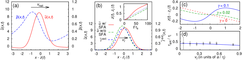
Figure 1: (color online) (a) The rescaled neuronal current, $\tilde{u}(x,t)$, and the rescaled inhibitory variable for SFA, $\tilde{p}(x,t)$ during a spontaneous motion in the moving frame centered at $z(t)$. $z(t)$ is the center of mass of $\tilde{u}(x,t)$. The $\tilde{u}(x,t)$ profile is moving to the direction pointed by the arrow. Parameters: $\tilde{k}$ (rescaled inhibition) = 0.5, $\gamma$ (SFA strength) = 0.2, $\tau_{{\rm s}}$ (time constant of neuronal current) = 1 ms and $\tau_{{\rm i}}$ (time constant of SFA) = 50 ms. (b) $\tilde{u}(x,t)$ and $\tilde{I}^{\text{ext}}(x,t)$, rescaled external stimulus, during a tracking process. Inset: $z_{0}(t)$ and $z(t)$, the centers of mass of $\tilde{I}^{\text{ext}}(x,t)$ and $\tilde{u}(x,t)$, respectively. The $\tilde{I}^{\text{ext}}(x,t)$ profile is moving in the direction of the arrow with velocity $v_{I}$. Parameters: $\tilde{k}=0.5$, $\gamma=0$, $\tau_{{\rm s}}=1\text{ ms}$, $\tilde{A}$ (rescaled magnitude of $\tilde{I}^{{\rm ext}}$) = 1.0 and $v_{I}=0.01$. (c) Displacement of the $\tilde{u}$ profile relative to the external stimulus, $z(t)-z_{0}(t)$. Parameters: $\tilde{k}=0.5$, $\tau_{{\rm i}}=50\text{ ms}$ and $\tau_{{\rm s}}=1\text{ ms}$. (d) Curve: The anticipation time, $\tau_{\text{ant}}\equiv\left[z(t)-z_{0}(t)\right]/v_{I}$, for the case with $\gamma=0.1$ in (c). Symbols: Anticipation time in Fig. 4 of Goodridge2000 with the assumption that $\tau_{i}=50$ ms and $a=22.5^{\circ}$.

IV Translational Invariance and Inversion Symmetry

Studies on neural field models showed that they can support a profile of localized activities even in the absence of external stimuli Wilson1972 ; Amari1977 ; Ben-Yishai1995 ; Fung2010 . Irrespective of the explicit form of this “bump”, it is sufficient to note that there exists a non-trivial stable solution $\{u_{0},p_{0}\}$ satisfying

$$F_{u}[x;u_{0},p_{0}]=F_{p}[x;u_{0},p_{0}]=0,$$ (13)

and that this solution is neutrally stable in $x$, that is, for an arbitrary bump position $z$,

$$F_{u}[x-z;u_{0},p_{0}]=F_{p}[x-z;u_{0},p_{0}]=0.$$ (14)

To study the stability issue of stationary state $(u_{0},p_{0})$, we consider the dynamics of the fluctuations about the steady state,

$$\frac{\partial}{\partial t}\delta u\left(x\right) =\int dx^{\prime}\frac{\partial F_{u}\left(x\right)}{\partial u\left(x^{\prime}\right)}\delta u\left(x^{\prime}\right)+\int dx^{\prime}\frac{\partial F_{u}\left(x\right)}{\partial p\left(x^{\prime}\right)}\delta p\left(x^{\prime}\right),$$ (15)

$$\frac{\partial}{\partial t}\delta p\left(x\right) =\int dx^{\prime}\frac{\partial F_{p}\left(x\right)}{\partial u\left(x^{\prime}\right)}\delta u\left(x^{\prime}\right)+\int dx^{\prime}\frac{\partial F_{p}\left(x\right)}{\partial p\left(x^{\prime}\right)}\delta p\left(x^{\prime}\right).$$ (16)

Here $\delta u(x)\equiv u(x)-u_{0}(x)$ and $\delta p(x)\equiv p(x)-p_{0}(x)$. Consider the solutions of these equations with time dependence $\exp(-\lambda t)$. Then the eigenvalue equations become the $\Delta x\rightarrow 0$ limit of the matrix eigenvalue equation

$$\left(\begin{array}[]{cc}\left\{\frac{\partial F_{u}\left(x_{i}\right)}{\partial u\left(x_{j}\right)}\right\}&\left\{\frac{\partial F_{u}\left(x_{i}\right)}{\partial p\left(x_{j}\right)}\right\}\\ \left\{\frac{\partial F_{p}\left(x_{i}\right)}{\partial u\left(x_{j}\right)}\right\}&\left\{\frac{\partial F_{p}\left(x_{i}\right)}{\partial p\left(x_{j}\right)}\right\}\end{array}\right)\left(\begin{array}[]{c}\left\{f_{u}\left(x_{j}\right)\right\}\\ \left\{f_{p}\left(x_{j}\right)\right\}\end{array}\right)\Delta x$$ (21)

$$= -\lambda\left(\begin{array}[]{c}\left\{f_{u}\left(x_{i}\right)\right\}\\ \left\{f_{p}\left(x_{i}\right)\right\}\end{array}\right).$$ (24)

The left eigenvector with the same eigenvalue is given by

$$\left(\begin{array}[]{cc}\left\{g_{u}\left(x_{j}\right)\right\}&\left\{g_{p}\left(x_{j}\right)\right\}\end{array}\right)\left(\begin{array}[]{cc}\left\{\frac{\partial F_{u}\left(x_{i}\right)}{\partial u\left(x_{j}\right)}\right\}&\left\{\frac{\partial F_{u}\left(x_{i}\right)}{\partial p\left(x_{j}\right)}\right\}\\ \left\{\frac{\partial F_{p}\left(x_{i}\right)}{\partial u\left(x_{j}\right)}\right\}&\left\{\frac{\partial F_{p}\left(x_{i}\right)}{\partial p\left(x_{j}\right)}\right\}\end{array}\right)\Delta x$$ (28)

$$= -\lambda\left(\begin{array}[]{cc}\left\{g_{u}\left(x_{i}\right)\right\}&\left\{g_{p}\left(x_{i}\right)\right\}\end{array}\right).$$ (30)

Translational invariance implies that $\partial u_{0}/\partial x$ and $\partial p_{0}/\partial x$ are the components of the right eigenfunction of the dynamical equations with eigenvalue 0, satisfying

$$\int dx^{\prime}\frac{\partial F_{u}\left(x\right)}{\partial u\left(x^{\prime}\right)}\frac{\partial u_{0}\left(x^{\prime}\right)}{\partial x^{\prime}}+\int dx^{\prime}\frac{\partial F_{u}\left(x\right)}{\partial p\left(x^{\prime}\right)}\frac{\partial p_{0}\left(x^{\prime}\right)}{\partial x^{\prime}}= \leavevmode\nobreak\ 0,$$ (31)

$$\int dx^{\prime}\frac{\partial F_{p}\left(x\right)}{\partial u\left(x^{\prime}\right)}\frac{\partial u_{0}\left(x^{\prime}\right)}{\partial x^{\prime}}+\int dx^{\prime}\frac{\partial F_{p}\left(x\right)}{\partial p\left(x^{\prime}\right)}\frac{\partial p_{0}\left(x^{\prime}\right)}{\partial x^{\prime}}= \leavevmode\nobreak\ 0.$$ (32)

The corresponding left eigenfunctions satisfy

$$\int dx^{\prime}g_{u}^{0}\left(x^{\prime}\right)\frac{\partial F_{u}\left(x^{\prime}\right)}{\partial u(x)}+\int dx^{\prime}g_{p}^{0}\left(x^{\prime}\right)\frac{\partial F_{p}\left(x^{\prime}\right)}{\partial u(x)} =\leavevmode\nobreak\ 0,$$ (33)

$$\int dx^{\prime}g_{u}^{0}\left(x^{\prime}\right)\frac{\partial F_{u}\left(x^{\prime}\right)}{\partial p(x)}+\int dx^{\prime}g_{p}^{0}\left(x^{\prime}\right)\frac{\partial F_{p}\left(x^{\prime}\right)}{\partial p(x)} =\leavevmode\nobreak\ 0.$$ (34)

For stable bumps, the eigenvalues of all other eigenfunctions are at most 0. Let $f_{u}^{n}$ and $f{}_{p}^{n}$ be the components of the eigenfunction with the $n^{{\rm th}}$ eigenvalue $-\lambda_{n}$, satisfying

$$\int dx^{\prime}\frac{\partial F_{u}\left(x\right)}{\partial u\left(x^{\prime}\right)}f_{u}^{n}\left(x^{\prime}\right)+\int dx^{\prime}\frac{\partial F_{u}\left(x\right)}{\partial p\left(x^{\prime}\right)}f_{p}^{n}\left(x^{\prime}\right)$$

$$=-\lambda_{n} f{}_{u}^{n}\left(x\right),$$ (35)

$$\int dx^{\prime}\frac{\partial F_{p}\left(x\right)}{\partial u\left(x^{\prime}\right)}f{}_{u}^{n}\left(x^{\prime}\right)+\int dx^{\prime}\frac{\partial F_{p}\left(x\right)}{\partial p\left(x^{\prime}\right)}f^{n}{}_{p}\left(x^{\prime}\right)$$

$$=-\lambda_{n} f_{p}^{n}\left(x\right).$$ (36)

Similarly, denoting the components of the left eigenfunctions as $g_{u}^{n}$ and $g_{p}^{n}$ respectively,

$$\int dx^{\prime}g_{u}^{n}\left(x^{\prime}\right)\frac{\partial F_{u}\left(x^{\prime}\right)}{\partial u(x)}+\int dx^{\prime}g_{p}^{n}\left(x^{\prime}\right)\frac{\partial F_{p}\left(x^{\prime}\right)}{\partial u(x)}$$

$$=-\lambda_{n} g_{u}^{n}\left(x\right),$$ (37)

$$\int dx^{\prime}g_{u}^{n}\left(x^{\prime}\right)\frac{\partial F_{u}\left(x^{\prime}\right)}{\partial p(x)}+\int dx^{\prime}g_{p}^{n}\left(x^{\prime}\right)\frac{\partial F_{p}\left(x^{\prime}\right)}{\partial p(x)}$$

$$=-\lambda_{n} g_{p}^{n}\left(x\right).$$ (38)

The eigenfunctions corresponding to eigenvalues $\lambda_{m}$ and $\lambda_{n}$ satisfy the orthogonality condition

$$\int dx^{\prime}g_{u}^{m}\left(x^{\prime}\right)f_{u}^{n}\left(x^{\prime}\right)+\int dx^{\prime}g_{p}^{m}\left(x^{\prime}\right)f_{p}^{n}\left(x^{\prime}\right)=\delta_{mn}.$$ (39)

For later use, we define

$$Q_{\psi\varphi}\equiv\int dxg_{\psi}^{0}\left(x\right)\int dx^{\prime}\frac{\partial F_{\psi}\left(x\right)}{\partial\varphi\left(x^{\prime}\right)}\frac{\partial\varphi_{0}\left(x^{\prime}\right)}{\partial x^{\prime}},$$ (40)

where $\psi,\varphi\in\{u,p\}$. The following identities are the results of translational invariance. Multiplying both sides of Eq. (31) by $g_{u}^{0}(x)$ and integrating over $x$, we obtain

$$Q_{uu}+Q_{up} =\leavevmode\nobreak\ 0.$$ (41)

Similarly, multiplying both sides of Eq. (32) by $g_{p}^{0}(x)$ and integrating over $x$, we have

$$Q_{pu}+Q_{pp} =\leavevmode\nobreak\ 0.$$ (42)

Likewise, from Eqs. (33) and (34), we find

$$Q_{uu}+Q_{pu}=Q_{up}+Q_{pp} =\leavevmode\nobreak\ 0.$$ (43)

Next, we consider the implications of inversion symmetry, that is, $\partial F_{\psi}\left(x\right)/\partial\varphi\left(x^{\prime}\right)=\partial F_{\psi}\left(-x\right)/\partial\varphi\left(-x^{\prime}\right)$ for $\psi,\varphi\in\{u,p\}$. Then the dynamics preserves parity. Suppose the bump state $u_{0}(x)$ and $p_{0}(x)$ has even parity. Then the distortion mode $\partial u_{0}/\partial x$ and $\partial p_{0}/\partial x$ has odd parity. Note that the corresponding left eigenfunctions $g_{u}^{0}$ and $g_{p}^{0}$ have the same parity as the right eigenfunctions.

V Intrinsic Behavior

Studies on neural field models with STD York2009 ; Fung2012 , SFA Coombes2005 and IFL Zhang2012 suggested that the network can support spontaneously moving profiles, even though there is no external moving input. This occurs when the static solution becomes unstable to positional displacement in some parameter regions. To study the stability issue of static solutions due to positional displacement, we consider

$$u\left(x,t\right) =u_{0}\left(x\right)+c_{0}\frac{\partial u_{0}\left(x\right)}{\partial x},$$ (44)

$$p\left(x,t\right) =p_{0}\left(x\right)+\varepsilon_{0}\frac{\partial p_{0}\left(x\right)}{\partial x}.$$ (45)

$c_{0}$ and $\varepsilon_{0}$ are the diplacements of the exposed and inhibitory profiles respectively (in the direction opposite to their signs). As derived in Appendix B, we have

$$\frac{d}{dt}\left(\varepsilon_{0}-c_{0}\right)=\lambda\left(\varepsilon_{0}-c_{0}\right),$$ (46)

where the instability eigenvalue $\lambda$ is given by

$$\lambda \equiv\frac{Q_{uu}}{I_{u}}+\frac{Q_{pp}}{I_{p}},$$ (47)

where $I_{\psi}=\int dxg_{\psi}^{0}(x)[d\psi_{0}(x)/dx]$ and $\psi\in\{u,p\}$. In the static phase, where stationary solutions are stable, $\lambda<0$. For systems with spontaneously moving bumps, $\lambda>0$. It implies that relative displacements of stationary $u_{0}$-profile and $p_{0}$-profile should diverge. The misalignment between the exposed $u_{0}$-profile and hidden $p_{0}$-profile will drive the motion of $u$ to sweep throughout the preferred stimulus space.

When the bump becomes translationally unstable, it moves with an intrinsic speed (or natural speed). To investigate the intrinsic speed denoted as $v_{{\rm nat}}$, we need to expand the dynamical equations beyond first order. The small parameter is the non-vanishing profile separation $\varepsilon_{0}$, now denoted as the intrinsic separation $\varepsilon_{{\rm int}}$. The critical regime is given by $\varepsilon_{{\rm int}}\sim\sqrt{\lambda}$. As derived in Appendix C,

$$v_{{\rm nat}}=\frac{\varepsilon_{{\rm int}}}{\tau_{{\rm int}}},$$ (48)

where

$$\tau_{{\rm int}}=-\frac{I_{p}}{Q_{pp}}.$$ (49)

We interpret $\tau_{{\rm int}}$ as the intrinsic time scale of the system. (We note in passing that the same result can be obtained by substituting the moving bump solution $u(x,t)=u_{0}(x-v_{{\rm nat}}t)$, $p(x,t)=p_{0}(x-v_{{\rm nat}}t+\varepsilon_{{\rm int}})$ into Eqs. (1) and (2) and expanding to the lowest order as was done in Eq. (46). However, such a derivation has not taken into account the stability of the solution.)

Noting that Eq. (48) also holds in the static phase with $v_{{\rm nat}}=\varepsilon_{{\rm int}}=0$, we infer that the separation of the exposed and inhibitory profiles is the cause of the spontaneous motion. The physical picture is that when the inhibitory profile lags behind the exposed profile, the neuronal activity will have a stronger tendency to shift away from the strongly inhibited region.

An example of the spontaneously moving state of neural field model with SFA is shown in Fig. 1(a), in which the $u$-profile and $p$-profile are plotted relative to the center of mass of $u$, $z(t)$. At the steady state of the spontaneously moving state, the $u$-profile moves in the direction opposite to the direction the $p$-profile biased to. So the $p$-profile always lags behind the $u$-profile during the spontaneous motion, while $u$-profile keeps moving due to the asymmetry granted by the misalignment between $u$ and $p$.

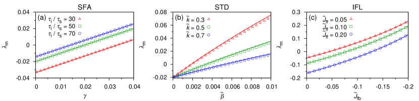
Figure 2: (color online) The exponential rates of small displacements of the $u$-profile from the $p$-profile, $\lambda$ for (a) SFA, (b) STD and (c) IFL. Symbols: simulations with various combinations of parameters. Curves: prediction by Eq. (46). Parameters: (a) $\tilde{k}=0.3$, (b) $\tau_{{\rm d}}=50\tau_{{\rm s}}$ and (c) $\tilde{k}=0.3$ and $\tau_{2}=\tau_{1}$.

We have tested the prediction of Eq. (46) with the three example models. In Fig. 2 there are simulation results (symbols) plotted with the corresponding predictions (curves), Eq. (47). In simulations the $p$-profile was intentionally displaced by a tiny displacement from the $u$-profile after the system has reached a stationary state. By monitoring the evolution of the displacement, $\lambda$ can be measured. They agree with the prediction very well. We can see that for small $\gamma$, $\tilde{\beta}$ and $-\tilde{J}_{{\rm fb}}$, the displacement will decay to zero eventually. But if these parameters are large enough, the tiny initial displacement will diverge. This divergence of the displacement will eventually lead to spontaneous motion. The results for SFA agree with those reported by Mi et al. Mi2014 , in which the system is able to support spontaneously moving network state only when $\gamma>\tau_{s}/\tau_{i}$.

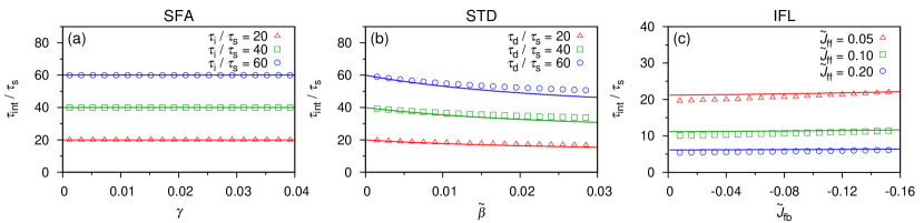
Figure 3: (color online) Comparison of the intrinsic time scale measured with a moving stimulus probe (symbols) and theoretically predicted (lines) for (a) SFA, (b) STD and (c) IFL. Parameters: (a) – (c) $\tilde{k}=0.3$ and $\hat{A}=0.25$.

VI Extrinsic Behavior

In the presence of a weak and slow external stimulus, we consider

$$u\left(x,t\right) =u_{0}\left(x-v_{I}t\right),$$ (50)

$$p\left(x,t\right) =p_{0}\left(x-v_{I}t\right)+\varepsilon_{0}\frac{dp_{0}(x-v_{I}t)}{dx},$$ (51)

$$I^{{\rm ext}}\left(x,t\right) =\frac{\max_{x}u(x,t)}{\tau_{{\rm stim}}}\exp\left(-\frac{\left|x-v_{I}t+s\right|^{2}}{4a^{2}}\right).$$ (52)

Here $\tau_{{\rm stim}}$ is referred to as the stimulus time, representing the time scale for the stimulus to produce significant response from the exposed profile. $s$ is the displacement of the bump relative to the stimulus. Substituting these assumptions into Eqs. (1) and (2), we find that at the steady state of the weak and slow stimulus limit, the separation $\varepsilon_{0}$ of the exposed and inhibitory profiles is given by $\varepsilon_{0}=v_{I}\tau_{{\rm int}}$ to the lowest order, as derived in Appendix D. Since both $v_{I}$ and $\varepsilon_{0}$ can be measured in simulations, this provides a way to test the validity of the theory. Indeed, simulations show that $\varepsilon_{0}$ is linearly proportional to $v_{I}$, so that the slope can be compared with the theoretical predictions of $\tau_{{\rm int}}$ by Eq. (49). Results shown in Fig. 3 for SFA, STD and IFL indicate excellent agreement with theoretical predictions.

We further note that in Fig. 3, the values of $\tau_{{\rm int}}$ have been obtained for low values of $\gamma$, $\tilde{\beta}$ and $-\tilde{J}_{{\rm fb}}$ where the bumps are intrinsically static. A difference between the moving and static phases is that $\tau_{{\rm int}}$ can be deduced in the former via Eq. (49) whereas the deduction is not possible in the latter since $v_{{\rm nat}}=0$. Hence Fig. 3 illustrates the close relation between $\tau_{{\rm int}}$ measured extrinsically and intrinsically, and that intrinsically inaccessible quantities can be obtained from extrinsic measurements.

More relevant to the anticipatory phenomenon, we are interested in the displacement $s$ and the anticipatory time $\tau_{{\rm ant}}$ of the exposed profile relative to the stimulus profile, given by

$$\tau_{{\rm ant}}\equiv\frac{s}{v_{I}}=\tau_{{\rm stim}}\tau_{{\rm int}}\lambda.$$ (53)

The derivation can be found in Appendix D. Hence $\tau_{{\rm int}}$ and $\lambda$ have the same sign. In the static phase, $\lambda<0$ implies that the tracking is delayed with $\tau_{{\rm ant}}<0$, whereas in the moving phase, $\lambda>0$ implies that the tracking is anticipatory with $\tau_{{\rm ant}}>0$. At the phase boundary, $\lambda=0$ and the system is in the ready-to-go state; here $\tau_{{\rm ant}}=0$ and the tracking is perfect.

Note that Eq. (53) is a manifestation of FRR, since it relates the instability parameter $\lambda$, as an intrinsic property, to the anticipatory time $\tau_{{\rm ant}}$, as an extrinsic property. To see how this relation is consistent with traditional fluctuation-response relations, one should note that $\tau_{\rm ant}^{-1}$ describes the rate of response of the system to moving stimuli, and $\lambda^{-1}$ is proportional to fluctuations in both static and moving phases, as derived in Appendix E.

For the example of the neural field with SFA in Fig. 1(a), the lag of the inhibitory profile $\tilde{p}$ drives the exposed profile $\tilde{u}$ to move in the direction with smaller $\tilde{p}$ (pointed by the arrow), as $\tilde{p}$ inhibits $\tilde{u}$.

In the absence of SFA, the bell-shaped attractor state of $\tilde{u}$ centered at $z(t)$ (shown in Fig. 1(b) as the green dashed line) lags behind a continuously moving stimulus $z_{I}\left(t\right)$ (shown as the blue dotted line). In the inset of Fig. 1(b), the lag of the network response develops after the stimulus starts to move and becomes steady after a while. In contrast, when SFA is sufficiently strong, the bump can track the stimulus at an advanced position (red solid curve in Fig. 1(b)). In this case, this tracking process anticipates the continuously moving stimulus. This behavior for SFA with various $\gamma$ and $v_{I}$ is summarized in Fig. 1(c).

Furthermore, the anticipation time is effectively constant in a considerable range of the stimulus speed. There is an obvious advantage for the brain to compensate delays with a constant leading time independent of the stimulus speed. To put the speed independence of $\tau_{{\rm ant}}$ in a perspective, we note that $\varepsilon_{0}=v_{I}\tau_{{\rm int}}$, implying that $\tau_{{\rm ant}}=\lambda\tau_{{\rm stim}}\varepsilon_{0}/v_{I}$. This shows that while the stimulus speed increases, the lag of the inhibitory profile behind the exposed profile also increases, providing an increasing driving force for the bump such that the anticipatory time remains constant.

This is confirmed when the SFA strength $\gamma$ is strong enough. As shown in Fig. 1(c) for $\gamma=0.1$, there is a velocity range such that the displacement of the center of mass relative to the stimulus, $z(t)-z_{I}(t)$, is directly proportional to the stimulus velocity. Thus the anticipation time $\tau_{{\rm ant}}\equiv(z-z_{I})/v_{I}$, given by the slope of the curve, is effectively constant. In Fig. 1(d), the anticipatory time is roughly 0.3$\tau_{{\rm i}}$ ($\tau_{{\rm i}}$ is the time constant of SFA) for a range of stimulus velocity, and has a remarkable fit with data from rodent experiments Goodridge2000 . This behavior can also be observed in neural field models with STD Fung2013 .

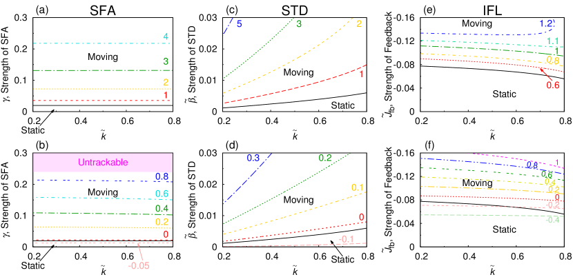
Figure 4: (color online) (a) Contours of intrinsic speed in the phase diagram of a neural field model with SFA. (b) Contours of anticipation time of a neural field model with SFA. (c) Same as (a), but for STD. (d) Same as (b), but for STD. (e) Same as (a), but for IFL. (f) Same as (b), but for IFL. Color curves: contours of intrinsic speed ((a), (c) & (e)), anticipatory time ((b), (d) & (f)). Number labels: values of the corresponding contour, in units of (a) $a/\tau_{{\rm i}}$, (b) $\tau_{{\rm i}}$, (c) $a/\tau_{{\rm d}}$, (d) $\tau_{{\rm d}}$ (e) $\tau_{2}/\tilde{J}_{{\rm ff}}$ and (f) $a/(\tau_{2}/\tilde{J}_{{\rm ff}})$. Black curves: phase boundaries separating the static, moving, and silent phases. Parameters: (a) $\tau_{{\rm i}}=50\tau_{{\rm s}}$. (b) $\hat{A}=0.25$, $v_{I}=0.002a/\tau_{{\rm s}}$ and $\tau_{{\rm i}}=50\tau_{{\rm s}}$. (c) $\tau_{{\rm d}}$ (time constant of STD) $=50\tau_{{\rm s}}$. (d) $\hat{A}=0.25$, $v_{I}=0.002a/\tau_{{\rm s}}$ and $\tau_{{\rm d}}=50\tau_{{\rm s}}$. (e) $\tilde{J}_{{\rm ff}}=0.1$ and $\tau_{1}$ (time constant of the primary layer) $=\tau_{2}$ (time constant of the hidden layer) $=\tau_{{\rm s}}$, (f) $\tilde{J}_{{\rm ff}}=0.1$, $\hat{A}=0.1$, $v_{I}=0.002a/\tau_{{\rm s}}$, $\tau_{1}=\tau_{2}$. In the shaded area of (b), $\hat{A}$ is too small to stabilize the system. One should note that metastatic phase reported in Fung2012 for STD are omitted in the current study, as the major concern in the paper is the relation between translational intrinsic behavior and translational extrinsic behavior.

The interdependency of anticipatory tracking dynamics and intrinsic dynamics in the framework of FRR is further illustrated by the relation between the anticipatory time and the intrinsic speed of spontaneous motions. Near the boundary of the moving phase, it is derived in Appendix D that

$$\tau_{{\rm ant}}=K\tau_{{\rm stim}}\tau_{{\rm int}}\left(v_{{\rm nat}}^{2}-v_{I}^{2}\right)+\tau_{{\rm con}},$$ (54)

or the quadratic relation in the limit of weak and slow stimulus

$$\tau_{{\rm ant}}=K\tau_{{\rm stim}}\tau_{{\rm int}}v_{{\rm nat}}^{2},$$ (55)

where $K$ and $\tau_{{\rm con}}$ are constants defined in Appendix D. Since all parameters besides $v_{{\rm nat}}^{2}$ and $v_{I}^{2}$ (taken to approach 0) are mostly slowly changing functions of system parameters, the contours of $v_{{\rm nat}}$ and $\tau_{{\rm ant}}$ in the parameter space have a one-to-one correspondence. The case for SFA is illustrated in Fig. 4(a) and (b).

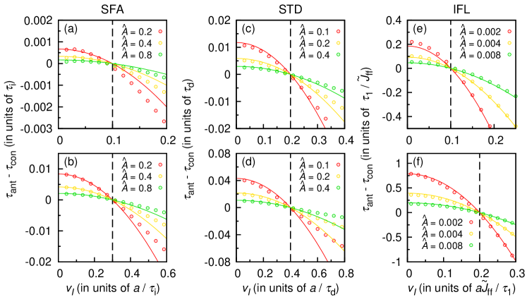
Figure 5: (color online) Anticipatory time versus the speed of the stimulus $v$. Black dashed lines: intrinsic speed of the corresponding set of parameters. Parameters: (a) $\tilde{k}=0.3$, $\gamma=0.0202$, $\tau_{i}=50\tau_{s}$ and $\hat{A}$ is labeled along with curves. (b) $\tilde{k}=0.3$, $\gamma=0.0217$,and $\tau_{i}=50\tau_{s}$. (c) $\tilde{k}=0.3$, $\tilde{\beta}=0.00198$ and $\tau_{{\rm d}}=50\tau_{s}$. (d) $\tilde{k}=0.3$, $\tilde{\beta}=0.00231$ and $\tau_{{\rm d}}=50\tau_{s}$. (e) $\tilde{k}=0.6$, $\tilde{J}_{{\rm fb}}=-0.0698$ and $\tau_{2}=\tau_{1}$. (f) $\tilde{k}=0.6$, $\tilde{J}_{{\rm fb}}=-0.0705$ and $\tau_{2}=\tau_{1}$.

Since these phenomena depend on the underlying symmetry of the system and its response to weak stimuli, they are expected to be observed in networks with the same symmetry as SFA networks. The correspondence between intrinsic motion and anticipation has been described in the specific case of STD networks Fung2013 . Comparable contour plots to Fig. 4(a) and (b) for STD are shown in 4(c) and (d), respectively. Similar phenomena can be found in Fig. 4(e) and (f) for IFL, except that the contours in Fig. 4 are distorted in the proximity of the repulsive phase (Repulsive phase can be observed if $(-\tilde{J}_{{\rm fb}})\gg\tilde{J}_{{\rm ff}}$, see Appendix A for more details). A minor discrepancy is that the contour for zero anticipatory time does not coincide perfectly with the phase boundary separating the moving and static phases. This is due to deviations from the weak input limit, since a finite input amplitude is necessary to prevent the network state from becoming “untrackable”. For SFA, the untrackable region is shaded in Fig. 4(b). For IFL, the untrackable region is located immediately beyond the upper right corner of Fig. 4(f).

VII Natural Tracking

For non-vanishing stimulus velocities in the moving phase, Eq. (54) predicts another interesting phenomenon linking tracking dynamics and intrinsic dynamics. When the stimulus is moving at the natural speed, i.e. $v_{I}=v_{{\rm nat}}$, the anticipatory time becomes independent of the strength of the external input which determines $\tau_{{\rm stim}}$, and the anticipation time curves are confluent at the value $\tau_{{\rm ant}}=\tau_{{\rm con}}$. This phenomenon for a particular neural field model with STD has been reported in Fung2013 ; here we show that it is generic in an entire family of neural fields.

The physical picture of this confluent behavior is that the stimulus plays two roles in driving the moving bump. First, it is used to drive the bump at the stimulus speed, if it is different from the intrinsic speed. Second, it is used to distort the shape of the bump. In the second role, the distortion is proportional to both the strength of the stimulus and the bump-stimulus displacement, $z(t)-z_{0}(t)$. Hence when the stimulus speed is the same as the intrinsic speed, the stimulus is primarily used to distort the bump shape. At the steady state, the bump-stimulus displacement is determined by the distortion per unit stimulus strength, which becomes independent of stimulus strength.

Since this phenomenon is based on a generic mechanism, it can be observed in all neural field models considered in this paper. Fig. 5 shows the simulation results in neural field models with SFA, STD and IFL. Fig. 5(a) shows the displacements in the SFA neural field model with the intrinsic speed $v_{{\rm nat}}=0.1a/\tau_{{\rm i}}$, where $\tau_{{\rm i}}$ is the SFA time scale. $\tau_{{\rm ant}}$-$v_{I}$ curves corresponding to different stimulus amplitudes intersect at $\tau_{{\rm i}}v_{{\rm nat}}/a=0.1$. Similar behaviors are shown in Fig. 5(b) for $v_{{\rm nat}}=0.3a/\tau_{{\rm i}}$, in Fig. 5(c) and (d) for STD, and in Fig. 5(e) and (f) for IFL. Remarkably, the confluent behavior remains valid even when the curves deviate from the parabolic shape predicted by Eq. (54).

VIII Noise Response

To further illustrate FRR, we consider the correlation between fluctuations due to noise in the absence of external input and the anticipatory time reacting to a weak and slow moving stimulus. This can be done by replacing $I^{{\rm ext}}$ in Eq. (1) with displacement noise $\xi\left(x,t\right)\equiv\eta\left(t\right)\partial u_{0}/\partial x$, where $\left\langle\eta\left(t\right)\right\rangle=0$ and $\left\langle\eta\left(t\right)\eta\left(t^{\prime}\right)\right\rangle=2T\delta\left(t-t^{\prime}\right)$. Analysis in Appendix E shows that for weak and slow stimuli,

$$\frac{\left\langle\delta\varepsilon_{0}^{2}\right\rangle}{T}=\begin{dcases}-\frac{\tau_{{\rm stim}}\tau_{{\rm int}}}{\tau_{{\rm ant}}-\tau_{{\rm con}}},&\mbox{for static phase,}\\ \frac{\tau_{{\rm stim}}\tau_{{\rm int}}}{2(\tau_{{\rm ant}}-\tau_{{\rm con}})},&\mbox{for moving phase.}\end{dcases}$$ (56)

Here, $\langle\delta\varepsilon_{0}^{2}\rangle$ represents the fluctuations of the lag of the inhibitory profile $p(x,t)$ behind the exposed profile $u(x,t)$ in response to the displacement noise.

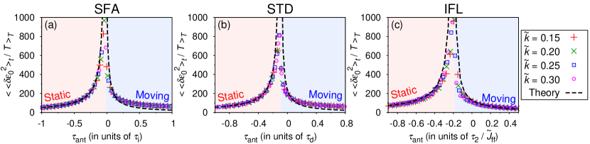
Figure 6: (color online) Intrinsic noise response of the system, $\left\langle\left\langle\delta\varepsilon_{0}^{2}\right\rangle_{t}/T\right\rangle_{T}$, versus anticipation time, $\tau_{{\rm ant}}$. Parameters: (a) $\hat{A}=0.02$ and $\tau_{i}=50\tau_{s}$. (c) $\hat{A}=0.02$ and $\tau_{d}=50\tau_{s}$. (b) $\hat{A}=0.02$, $\tilde{J}_{{\rm ff}}=0.1$ and $\tau_{2}=\tau_{1}$.

The behavior predicted by Eq. (56) can be seen from simulations. The numerical procedure is explained in Appendix F. In Fig. 6, there are two branches in each sub-figure. The branches for $\tau_{{\rm ant}}>\tau_{{\rm con}}$ and $\tau_{{\rm ant}}<\tau_{{\rm con}}$ correspond to the moving and static phases respectively. Remarkably, data points with different network parameters collapse onto common curves. The fluctuations are divergent at the confluence point predicted by Eq. (54). The regimes of $\tau_{{\rm ant}}>0$ and $\tau_{{\rm ant}}<0$, corresponding to anticipatory and delayed tracking respectively, effectively coincide with the two branches in the limit of weak stimuli, since at the confluence point the instability eigenvalue $\lambda=(\tau_{{\rm ant}}-\tau_{{\rm con}})/(\tau_{{\rm stim}}\tau_{{\rm int}})$ approaches 0 in that limit.

IX Conclusion

Many intriguing dynamical behaviors of physical systems can be understood from the relationship between the fluctuation properties of a system near equilibrium and its response to external driving fields, namely, the FRR Einstein1905 ; vonSmoluchowski1906 ; Nyquist1928 ; Huang1987 . Here, we show that the same idea is applicable to understanding the dynamics of neural fields. In particular, we have found a fluctuation-response relation for neural fields processing dynamical information. Traditionally, theoretical techniques based on equilibrium concepts have been well developed in analyzing neural fields processing static information. On the other hand, neural fields responding to external dynamical information are driven to near-equilibrium states, and FRRs are suitable tools to describe their behaviors.

There have been previous analyses on neural fields with slow, localized inhibitory feedbacks. Moving phases and anticipatory tracking have been studied in neural fields with STD York2009 ; Fung2012 ; Fung2013 ; Fung2015 , SFA Mi2014 ; Fung2015 and IFL Ben-Yishai1997 ; Zhang2012 . However, results of the boundary between the static and moving phases, the intrinsic speed or the tracking delay were specific to the particular models, concealing their common underlying physical principles.

The unification of these various manifestations were provided by the FRR considered in this paper. We pointed out that they have a common structure consisting of an exposed variable ($u$) coupled to external stimuli and an inhibitory variable ($p$) hidden from stimuli. Irrespective of the explicit form of the dynamical equations, the FRR is generically based on (i) the existence of a non-zero solution, and (ii) this solution is translationally invariant and (iii) possesses inversion symmetry. Consequently, FRR is able to relate (i) the positional stability of the activity states, to (ii) their lagging/leading position relative to external stimuli during tracking, and to (iii) fluctuations due to thermal noises.

Particularly relevant to the processing of motional information, FRR predicts that the regimes of anticipatory and delayed tracking effectively coincide with the regimes of moving and static phases respectively, and that the anticipation time becomes independent of stimulus speed for slow and weak stimuli, and independent of stimulus amplitude when the stimulus moves at the intrinsic speed.

This brings FRR into contact with experimental observations of how neural systems cope with time delays in the transmission and processing of signals, which are ubiquitous in neural systems. To compensate for delays, neural systems need to anticipate moving stimuli, which has been observed in HD cells of rodents Goodridge2000 . FRR provides the condition for the anticipatory behavior. Furthermore, we predict that the anticipatory time is independent of the stimulus speed, offering the advantage of a fixed time for the system to respond.

FRR also provides a means to measure quantities that are normally inaccessible in certain regimes. For example, the intrinsic time in the static phase is intrinsically unmeasurable since there is no separation between the exposed and inhibitory profiles in that phase. Our analysis shows that the intrinsic time is identical to the local time lapse between the exposed and inhibitory profiles due to moving stimuli, thus providing an extrinsic instrument to measure the intrinsic time.

Since FRR is successful in unifying the behaviors of neural fields with slow inhibitory feedback mechanisms such as STD, SFA, IFL and other neural fields of the family, it can be extended to study the relation between fluctuations and responses in other modes of encoding information, such as amplitude fluctuations and amplitude responses. It is expected to be an important element in understanding the processing of dynamical information in the brain. It can also be applied to other natural or artificial dynamical systems in which motional information needs to be processed in real time, and FRR provides a powerful tool to analyze the dynamical properties of these systems.

Appendix A Intrinsic Behaviors of Inhibitory Feedback Loops

This is one of the three examples mentioned in the main text. For the other two examples, a detailed study on CANNs with STD can be found in Fung2012 , and the intrinsic behavior of CANNs with SFA is similar. In this section, the intrinsic behaviors of a bump-shaped profile in a two-layered network with an inhibitory feedback loop (IFL) are summarized.

If the negative feedback strength ($\tilde{J}_{{\rm fb}}$) is strong enough, the bump in the second layer that provides a negative feedback to the first layer can destabilize the bump in the first layer. At the steady state, the misalignment between two profiles becomes a constant. As shown in Fig. A.1, the two misaligned bumps move spontaneously. Since the neurons in the first layer receive negative feedbacks and neurons in the second layer receives positive feedforwards, the magnitude of $\tilde{p}$-profile is larger than $\tilde{u}$-profile.

The intrinsic behavior supported by the system is determined by the choice of parameters. Figure A.2 shows the typical cases of the static phase, the moving phase and the repulsive phase. In simulations, the initi al conditions of $\tilde{u}$ and $\tilde{p}$ are misaligned so that the environment of $\tilde{u}$ is not symmetric about its center. If the magnitude of $\tilde{J}_{{\rm fb}}$ is not strong enough, the bump will relax to a static state, see Fig. A.2 (a) and (b). For a sufficiently strong $\tilde{J}_{{\rm fb}}$, the bump can move spontaneously as in Fig. A.1 and Fig. A.2 (c) and (d). This is the moving phase. In this phase, the $\tilde{p}$-profile repels the $\tilde{u}$-profile. However, at the same time, the $\tilde{u}$-profile attracts the $\tilde{p}$-profile. So, at the equilibrium state, the misalignment between two profiles becomes steady.

If $\tilde{J}_{{\rm fb}}$ is too strong, the spontaneous motion will terminate. In this case, initially, the $\tilde{p}$-profile repels the $\tilde{u}$-profile and the $\tilde{u}$-profile attracts the $\tilde{p}$-profile. However, in the repulsive phase, the repulsion is so strong that the attraction can no longer balance the repulsive force. As a result, the two profiles move apart out of the interactive range of each other, as shown in Fig. A.2 (e) and (f). The spontaneous motion cannot sustain at the steady state. In general, together with the trivial solution, there are four phases in two-layer CANNs, under the current setting. The phase diagram for these four phases is shown in the main paper.

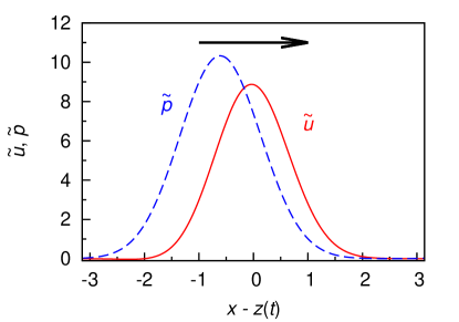
Figure A.1: (color online) A snapshot of the network state of a two-layered network in its moving phase. $\tilde{u}$ and $\tilde{p}$ are the rescaled neuronal current profile of the first and second layers respectively. The profiles are moving in the direction of the arrow at the top. Parameters: $\tilde{k}=0.5$, $\tilde{J}_{{\rm ff}}=0.1$, $\tilde{J}_{{\rm fb}}=-0.1$ and $\tau_{2}=\tau_{1}=1$.

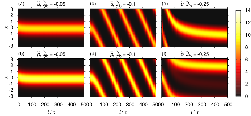
Figure A.2: (color online) Typical examples of network behaviors for various phases: static phase, moving phase and repulsive phase. (a) and (b): static phase. (c) and (d): moving phase. (e) and (f): repulsive phase. Parameters: $\tilde{k}=0.5$, $\tilde{J}_{{\rm ff}}=0.1$ and $\tau_{2}=\tau_{1}=1$.

The slowness of the inhibitory feedback, and hence the existence of the moving phase, arises from the weak coupling between the exposed and inhibitory layers. To see this, we consider the moving bump solution

$$u(x,t) =u^{0}\exp\left[-\frac{(x-vt)^{2}}{4a^{2}}\right],\quad\mathrm{and}$$ (57)

$$p(x,t) =p^{0}\exp\left[-\frac{(x-vt+s)^{2}}{4a^{2}}\right].$$ (58)

Substituting into Eq. (1), multiplying both sides by $\exp[-(x-vt)^{2}/(4a^{2})]/\sqrt{2\pi a^{2}}$ and integrating,

$$\tilde{u}^{0}=\frac{\left.\tilde{u}^{0}\right.^{2}}{\sqrt{2}B_{u}}+\tilde{J}_{\mathrm{fb}}\frac{\left.\tilde{p}^{0}\right.^{2}}{\sqrt{2}B_{p}}e^{-\frac{s^{2}}{8a^{2}}},$$ (59)

where $B_{u}=1+\tilde{k}\left.\tilde{u}^{0}\right.^{2}/8$ and $B_{p}=1+\tilde{k}\left.\tilde{p}^{0}\right.^{2}/8$.

Substituting into Eq. (1), multiplying both sides by $[(x-vt)/a]\exp[-(x-vt)^{2}/(4a^{2})]/\sqrt{2\pi a^{2}}$ and integrating,

$$\frac{v\tau_{1}}{2a}\tilde{p}^{0}=-\tilde{J}_{{\rm fb}}\frac{\left.\tilde{p}^{0}\right.^{2}}{\sqrt{2}B_{p}}\frac{s}{2a}e^{-\frac{s^{2}}{8a^{2}}}.$$ (60)

Consider the condition for the moving phase boundary with both $v$ and $s$ approaching 0 at a finite ratio. The above equations imply that

$$\frac{v\tau_{1}}{s}=-\frac{\tilde{J}_{{\rm fb}}\frac{\left.\tilde{p}^{0}\right.^{2}}{\sqrt{2}B_{p}}}{\frac{\left.\tilde{u}^{2}\right.^{2}}{\sqrt{2}B_{u}}+\tilde{J}_{\mathrm{fb}}\frac{\left.\tilde{p}^{0}\right.^{2}}{\sqrt{2}B_{p}}}\sim-\frac{\tilde{J}_{{\rm fb}}}{1+\tilde{J}_{{\rm fb}}}.$$ (61)

Similarly, by considering the dynamics of the second layer, we have

$$\frac{v\tau_{2}}{s}\sim\frac{\tilde{J}_{{\rm ff}}}{1+\tilde{J}_{{\rm ff}}}.$$ (62)

Hence weak interlayer couplings, $\left|\tilde{J}_{{\rm fb}}\right|\ll 1$ or $\tilde{J}_{{\rm ff}}\ll 1$ play the same role as the ratio $\tau_{{\rm s}}/\tau_{{\rm d}}$ in STD Fung2012 .

Appendix B Intrinsic Behavior of Profile Separation

We consider perturbations that cause the exposed and inhibitory profiles to separate. These distortions have odd parity. To keep the discussions general, we further assume that distortion modes with even parity also contribute to the perturbations. As we shall see, the coupling of these even parity modes with the odd parity modes play a role in determining the intrinsic and extrinsic behaviors in the moving phase. Hence we consider perturbations of the form

$$\delta u\left(x\right)=c_{0}\frac{\partial u_{0}}{\partial x}+c_{1}u_{1}\left(x\right)\text{{\rm, }}\delta p\left(x\right)=\varepsilon_{0}\frac{\partial p_{0}}{\partial x}+\varepsilon_{1}p_{1}\left(x\right).$$ (63)

$c_{0}$ and $\varepsilon_{0}$ are considered to be the displacement of the exposed and inhibitory profiles respectively (in the direction opposite to their signs). $u_{1}$ and $p_{1}$ are the most significant even parity distortion modes. They are substituted into the dynamical equations (LABEL:eq:depsilondcdt_a) and (73). Multiplying both sides of Eq. (LABEL:eq:depsilondcdt_a) by $g_{u}^{0}$ and integrating,

$${\rm LHS} =\frac{\partial c_{0}}{\partial t}\int dxg_{u}^{0}\left(x\right)\frac{\partial u_{0}}{\partial x}+\frac{\partial c_{1}}{\partial t}\int dxg_{u}^{0}\left(x\right)u_{1}\left(x\right)$$

$$=\frac{\partial c_{0}}{\partial t}I_{u},$$ (64)

where, for $i=u$, $p$,

$$I_{i}=\int dxg_{i}^{0}\left(x\right)\frac{\partial u_{i}^{0}}{\partial x},$$ (65)

Note that the second term in Eq. (64) vanishes since $g_{u}^{0}$ and $u_{1}$ have opposite parity. On the right hand side,

$${\rm RHS}_{1} =c_{0}\int dxg_{u}^{0}\left(x\right)\int dx^{\prime}\frac{\partial F_{u}\left(x\right)}{\partial u\left(x^{\prime}\right)}\frac{\partial u_{0}\left(x^{\prime}\right)}{\partial x^{\prime}}$$

$$+c_{1}\int dxg_{u}^{0}\left(x\right)\int dx^{\prime}\frac{\partial F_{u}\left(x\right)}{\partial u\left(x^{\prime}\right)}u_{1}\left(x^{\prime}\right).$$ (66)

The second term vanishes due to odd parity. Hence

$${\rm RHS}_{1}=c_{0}\int dxg_{u}^{0}\left(x\right)\int dx^{\prime}\frac{\partial F_{u}\left(x\right)}{\partial u\left(x^{\prime}\right)}\frac{\partial u_{0}\left(x^{\prime}\right)}{\partial x^{\prime}}=c_{0}Q_{uu}$$ (67)

Similarly, the second term on the right hand side becomes

$${\rm RHS}_{2}=\varepsilon_{0}\int dxg_{u}^{0}\left(x\right)\int dx^{\prime}\frac{\partial F_{u}\left(x\right)}{\partial p\left(x^{\prime}\right)}\frac{\partial p_{0}\left(x^{\prime}\right)}{\partial x^{\prime}}=\varepsilon_{0}Q_{up}.$$ (68)

Hence we obtain

$$I_{u}\frac{\partial c_{0}}{\partial t}=Q_{uu}c_{0}+Q_{up}\varepsilon_{0}.$$ (69)

Similarly, from Eq. (73),

$$I_{p}\frac{\partial\varepsilon_{0}}{\partial t}=Q_{pu}c_{0}+Q_{pp}\varepsilon_{0}.$$ (70)

Using the identities of translational invariance in Eqs. (86) and (87),

$$\frac{\partial}{\partial t}\left(\begin{array}[]{c}c_{0}\\ \varepsilon_{0}\end{array}\right)=\left(\begin{array}[]{cc}Q_{uu}/I_{u}&-Q_{uu}/I_{u}\\ -Q_{pp}/I_{p}&Q_{pp}/I_{p}\end{array}\right)\left(\begin{array}[]{c}c_{0}\\ \varepsilon_{0}\end{array}\right).$$ (71)

This implies

$$\frac{\partial}{\partial t}\left(\varepsilon_{0}-c_{0}\right) = \left(\frac{Q_{uu}}{I_{u}}+\frac{Q_{pp}}{I_{p}}\right)\left(\varepsilon_{0}-c_{0}\right),$$

$$\frac{\partial}{\partial t}\left(\frac{I_{u}}{Q_{uu}}c_{0}+\frac{I_{p}}{Q_{pp}}\varepsilon_{0}\right) = 0.$$ (73)

Eq. (LABEL:eq:depsilondcdt_a) describes the dynamics of the displacement of the inhibitory profile relative to the exposed profile. The instability eigenvalue in Eq. (LABEL:eq:depsilondcdt_a) is denoted as

$$\lambda\equiv\frac{Q_{uu}}{I_{u}}+\frac{Q_{pp}}{I_{p}}.$$ (74)

Appendix C Intrinsic Speed

When the bump becomes translationally unstable, it moves with an intrinsic speed (or natural speed). To investigate the intrinsic speed, we need to expand the dynamical equation beyond first order. In this case, the translational variables become coupled with the next eigenfunction. To keep the analysis trackable, we choose the coordinate with $c_{0}=0$. Near the phase boundary of the static and moving phases, $v_{\mathrm{nat}}\sim\varepsilon_{0}$ and $c_{1}\sim\varepsilon_{1}\sim\varepsilon_{0}^{2}$, as will be verified in this section. Hence to include third order terms, it is sufficient to consider terms in the dynamical equations containing $\varepsilon_{{\rm 0}}$, $c_{1}$, $\varepsilon_{1}$, $\varepsilon_{0}^{2}$, $\varepsilon_{{\rm 0}}c_{1}$, $\varepsilon_{0}\varepsilon_{1}$, $\varepsilon_{0}^{3}$, $v_{\mathrm{nat}}\varepsilon_{0}$, $v_{\mathrm{nat}}c_{1}$, $v_{\mathrm{nat}}\varepsilon_{1}$. Substituting Eq. (63) into the dynamical equation (LABEL:eq:depsilondcdt_a), expanding to third order for a bump moving with natural speed $v_{\mathrm{nat}}$, multiplying both sides of Eq. (LABEL:eq:depsilondcdt_a) by $g_{u}^{0}$ and integrating,

$$-I_{u}v_{\mathrm{nat}}-M_{u}v_{\mathrm{nat}}c_{1}=\leavevmode\nobreak\ Q_{up}\varepsilon_{{\rm 0}}+T_{upu}\varepsilon_{0}c_{1}+T_{upp}\varepsilon_{0}\varepsilon_{1}$$

$$+\frac{Q_{uppp}}{6}\varepsilon_{0}^{3},$$ (75)

where, for $i$, $j$, $k$, $l=u$, $p$,

$$M_{i} =\int dxg_{i}^{0}\frac{\partial u_{i}^{1}(x)}{\partial x},$$ (76)

$$T_{ijk} =\int dxg_{i}^{0}\left(x\right)\int dx_{1}\int dx_{2}$$

$$\qquad\qquad\frac{\partial^{2}F_{i}\left(x\right)}{\partial u_{j}\left(x_{1}\right)\partial u_{k}\left(x_{2}\right)}\frac{\partial u_{j}^{0}\left(x_{1}\right)}{\partial x_{1}}u_{k}^{1}(x_{2}),$$ (77)

$$Q_{ijkl} =\int dxg_{i}^{0}\left(x\right)\int dx_{1}\int dx_{2}\int dx_{3}$$

$$\qquad\qquad\frac{\partial^{3}F_{i}\left(x\right)}{\partial u_{j}\left(x_{1}\right)\partial u_{k}\left(x_{2}\right)\partial u_{l}\left(x_{3}\right)}\frac{\partial u_{j}^{0}\left(x_{1}\right)}{\partial x_{1}}$$

$$\qquad\qquad\qquad\frac{\partial u{}_{k}^{0}\left(x_{2}\right)}{\partial x_{2}}\frac{\partial u_{l}^{0}\left(x_{3}\right)}{\partial x_{3}}.$$ (78)

The left hand side of Eq. (75) arises from the time rate of change of the neural activities at a location when the bump passes by. These terms are proportional to the bump velocity and are referred to as the wave terms. Substituting Eq. (63) into the dynamical equation (LABEL:eq:depsilondcdt_a), multiplying both sides of Eq. (LABEL:eq:depsilondcdt_a) by $g_{u}^{1}$ and integrating,

$${\rm LHS}=\frac{\partial c_{1}}{\partial t}\int dxg_{u}^{1}\left(x\right)u_{1}\left(x\right)=\frac{\partial c_{1}}{\partial t}J_{u},$$ (79)

where, for $i=u$, $p$,

$$J_{i}=\int dxg_{i}^{1}\left(x\right)u_{i}^{1}\left(x\right),$$ (80)

with $u_{i}^{1}(x)$ representing the functions $u_{1}(x)$ and $p_{1}(x)$ for $i=u$, $p$ respectively. On the right hand side,

$${\rm RHS}= \leavevmode\nobreak\ c_{1}\int dxg_{u}^{1}\left(x\right)\int dx^{\prime}\frac{\partial F_{u}\left(x\right)}{\partial u\left(x^{\prime}\right)}u_{1}\left(x^{\prime}\right)$$

$$+\varepsilon_{1}\int dxg_{u}^{1}\left(x\right)\int dx^{\prime}\frac{\partial F_{u}\left(x\right)}{\partial p\left(x^{\prime}\right)}p_{1}\left(x^{\prime}\right)$$

$$+\frac{\varepsilon_{{\rm 0}}^{2}}{2}\int dx_{1}\int dx_{2}\frac{\partial^{2}F_{u}(x)}{\partial p(x_{1})\partial p(x_{2})}\frac{\partial p_{0}(x_{1})}{\partial x_{1}}\frac{\partial p_{0}(x_{2})}{\partial x_{2}}$$

$$= \leavevmode\nobreak\ c_{1}P_{uu}+\varepsilon_{1}P_{up}+\frac{S_{upp}}{2}\varepsilon_{{\rm 0}}^{2},$$ (81)

where, for $i$, $j$, $k=u$, $p$,

$$P_{ij}= \leavevmode\nobreak\ \int dxg_{i}^{1}\left(x\right)\int dx^{\prime}\frac{\partial F_{i}\left(x\right)}{\partial u_{j}\left(x^{\prime}\right)}u_{j}^{1}\left(x^{\prime}\right).$$ (82)

$$S_{ijk}= \leavevmode\nobreak\ \int dxg_{i}^{1}\left(x\right)\int dx_{1}\int dx_{2}\frac{\partial^{2}F_{i}\left(x\right)}{\partial u_{j}\left(x_{1}\right)\partial u_{k}\left(x_{2}\right)}$$

$$\qquad\qquad\qquad\qquad\qquad\quad\frac{\partial u_{j}^{0}\left(x_{1}\right)}{\partial x_{1}}\frac{\partial u_{k}^{0}\left(x_{2}\right)}{\partial x_{2}}.$$ (83)

Hence we obtain

$$J_{u}\frac{\partial c_{1}}{\partial t}=P_{uu}c_{1}+P_{up}\varepsilon_{1}+\frac{S_{upp}}{2}\varepsilon_{0}^{2}.$$ (84)

Similarly, from Eq. (73),

$$I_{p}\frac{\partial\varepsilon_{{\rm 0}}}{\partial t}-I_{p}v_{\mathrm{nat}}-M_{p}v_{\mathrm{nat}}\varepsilon_{1}= \leavevmode\nobreak\ Q_{pp}\varepsilon_{0}+T_{ppu}\varepsilon_{0}c_{1}$$

$$+T_{ppp}\varepsilon_{0}\varepsilon_{1}+\frac{Q_{pppp}}{6}\varepsilon_{0}^{3}.$$ (85)

$$J_{p}\frac{\partial\varepsilon_{1}}{\partial t}-K_{p}v_{\mathrm{nat}}\varepsilon_{{\rm 0}}= P_{pu}c_{1}+P_{pp}\varepsilon_{1}+\frac{S_{ppp}}{2}\varepsilon_{0}^{2},$$ (86)

where, for $i=u$, $p$,

$$K_{i}=\int dxg_{i}^{1}(x)\frac{\partial^{2}u_{i}^{0}(x)}{\partial x^{2}}.$$ (87)

Since the solution to the above equations will be tedious, it is instructive to interpret the equations from a symmetry point of view. This is because when there is a separation between the exposed and inhibitory profiles in the moving bump, the displacement mode will be coupled with other distortion modes that prevent the profile separation from diverging. Consider the coupling with the most important symmetric mode, which is the width mode for weak inhibition, and the height mode for strong inhibition Fung2010 . Irrespective of the details of these modes, we can summarize the steady state equations (75) and (85) as

$$-I_{u}v_{{\rm nat}}-M_{u}v_{{\rm nat}}c_{1}= \leavevmode\nobreak\ Q_{up}\varepsilon_{0}$$

$$+R_{u}\left(\varepsilon_{0}^{2},v_{{\rm nat}}\varepsilon_{0}\right)\varepsilon_{0},$$ (88)

$$-I_{p}v_{{\rm nat}}-M_{p}v_{{\rm nat}}\varepsilon_{1}= \leavevmode\nobreak\ Q_{pp}\varepsilon_{0}$$

$$+R_{p}\left(\varepsilon_{0}^{2},v_{{\rm nat}}\varepsilon_{0}\right)\varepsilon_{0}.$$ (89)

In Eq. (88), we interpret $R_{u}\varepsilon_{0}$ as the force acting on the displacement mode due to the coupling with the symmetric modes. Since the modes are decoupled when $\varepsilon_{0}$ vanishes, we consider forces proportional to $\varepsilon_{0}$. The magnitudes of $R_{u}$ and $R_{p}$ depend on the following two factors. (1) The distortions of the symmetric modes. Since the distortions of the symmetric modes should be the same for $+\varepsilon_{0}$ and $-\varepsilon_{0}$, they should be proportional to $\varepsilon_{0}^{2}$. (2) It should depend on the bump velocity via $v_{{\rm nat}}\varepsilon_{0}$, which originates from the wave terms of the moving symmetric mode.

Similarly, in the wave terms, $c_{1}$ and $\varepsilon_{1}$ can be expressed as a linear combination of $\varepsilon_{0}^{2}$ and $v_{{\rm nat}}\varepsilon_{0}$. Hence we can write

$$-I_{u}v_{{\rm nat}}-M_{u1}v_{{\rm nat}}\varepsilon_{0}^{2}-M_{u2}v_{{\rm nat}}^{2}\varepsilon_{0}$$

$$\qquad\qquad\qquad=Q_{up}\varepsilon_{0}+R_{u1}\varepsilon_{0}^{3}+R_{u2}v_{{\rm nat}}\varepsilon_{0}^{2},$$ (90)

$$-I_{p}v_{{\rm nat}}-M_{p1}v_{{\rm nat}}\varepsilon_{0}^{2}-M_{p2}v_{{\rm nat}}^{2}\varepsilon_{0}$$

$$\qquad\qquad\qquad=Q_{pp}\varepsilon_{0}+R_{p1}\varepsilon_{0}^{3}+R_{p2}v_{{\rm nat}}\varepsilon_{0}^{2}.$$ (91)

After elimination the variables $c_{1}$ and $\varepsilon_{1}$ using Eqs. (84) and (86), we obtain

$$R_{u1}= \leavevmode\nobreak\ \frac{T_{upu}\left(P_{up}S_{ppp}-P_{pp}S_{upp}\right)}{2\left(P_{uu}P_{pp}-P_{pu}P_{up}\right)}$$

$$+\frac{T_{upp}\left(P_{pu}S_{upp}-P_{uu}S_{ppp}\right)}{2\left(P_{uu}P_{pp}-P_{pu}P_{up}\right)}+\frac{Q_{uppp}}{6},$$ (92)

$$R_{u2}= \leavevmode\nobreak\ \frac{T_{upu}P_{up}K_{p}}{P_{uu}P_{pp}-P_{pu}P_{up}}-\frac{T_{upp}P_{uu}K_{p}}{P_{uu}P_{pp}-P_{pu}P_{up}},$$ (93)

$$R_{p1}= \leavevmode\nobreak\ \frac{T_{ppu}\left(P_{up}S_{ppp}-P_{pp}S_{upp}\right)}{2\left(P_{uu}P_{pp}-P_{pu}P_{up}\right)}+$$

$$\frac{T_{ppp}\left(P_{pu}S_{upp}-P_{uu}S_{ppp}\right)}{2\left(P_{uu}P_{pp}-P_{pu}P_{up}\right)}+\frac{Q_{pppp}}{6},$$ (94)

$$R_{p2}= \leavevmode\nobreak\ \frac{T_{ppu}P_{up}K_{p}}{P_{uu}P_{pp}-P_{pu}P_{up}}-\frac{T_{ppp}P_{uu}K_{p}}{P_{uu}P_{pp}-P_{pu}P_{up}},$$ (95)

$$M_{u1}= \leavevmode\nobreak\ \frac{M_{u}\left(P_{up}S_{ppp}-P_{pp}S_{upp}\right)}{2\left(P_{uu}P_{pp}-P_{pu}P_{up}\right)},$$ (96)

$$M_{u2}= \leavevmode\nobreak\ \frac{M_{u}P_{up}K_{p}}{P_{uu}P_{pp}-P_{pu}P_{up}},$$ (97)

$$M_{p1}= \leavevmode\nobreak\ \frac{M_{p}\left(P_{pu}S_{upp}-P_{uu}S_{ppp}\right)}{2\left(P_{uu}P_{pp}-P_{pu}P_{up}\right)},$$ (98)

$$M_{p2}= \leavevmode\nobreak\ -\frac{M_{p}P_{uu}K_{p}}{P_{uu}P_{pp}-P_{pu}P_{up}}.$$ (99)

In fact, the symmetric modes in Eqs. (90) and (91) may consist of more than one or even all of them. We note that the relaxation rate eigenvalues do not enter the equation here. From Eqs. (90) and (91),

$$-v_{{\rm nat}}= \leavevmode\nobreak\ \frac{Q_{up}\varepsilon_{0}}{I_{u}}+\frac{R_{u1}\varepsilon_{0}^{3}}{I_{u}}+\frac{R_{u2}v_{{\rm nat}}\varepsilon_{0}^{2}}{I_{u}}$$

$$\qquad\qquad+\frac{M_{u1}v_{{\rm nat}}\varepsilon_{0}^{2}}{I_{u}}+\frac{M_{u2}v_{{\rm nat}}^{2}\varepsilon_{0}}{I_{u}},$$ (100)

$$-v_{{\rm nat}}= \leavevmode\nobreak\ \frac{Q_{pp}\varepsilon_{0}}{I_{p}}+\frac{R_{p1}\varepsilon_{0}^{3}}{I_{p}}+\frac{R_{p2}v_{{\rm nat}}\varepsilon_{0}^{2}}{I_{p}}$$

$$\qquad\qquad+\frac{M_{p1}v_{{\rm nat}}\varepsilon_{0}^{2}}{I_{p}}+\frac{M_{p2}v_{{\rm nat}}^{2}\varepsilon_{0}}{I_{p}}.$$ (101)

Note that $Q_{uu}+Q_{up}=0$ due to translational invariance. Equating the two expressions of $v_{{\rm nat}}$, we arrive at an expression for $\varepsilon_{{\rm int}}$,

$$\left(\frac{Q_{uu}}{I_{u}}+\frac{Q_{pp}}{I_{p}}\right)\varepsilon_{{\rm int}}$$

$$= \leavevmode\nobreak\ \left(\frac{R_{u1}}{I_{u}}-\frac{R{}_{p1}}{I_{p}}\right)\varepsilon_{{\rm int}}^{3}$$

$$\qquad+\left(\frac{R_{u2}+M_{u1}}{I_{u}}-\frac{R{}_{p2}+M_{p2}}{I_{p}}\right)v_{{\rm nat}}\varepsilon_{{\rm int}}^{2}$$

$$\qquad+\left(\frac{M_{u2}}{I_{u}}-\frac{M_{p2}}{I_{p}}\right)v_{{\rm nat}}^{2}\varepsilon_{{\rm int}}.$$ (102)

Furthermore, from Eq. (85), we have, to the lowest order,

$$\varepsilon_{{\rm int}}\approx v_{{\rm nat}}\tau_{{\rm int}},\quad\tau_{\mathrm{int}}\equiv-\frac{I_{p}}{Q_{pp}}.$$ (103)

$\tau_{\mathrm{int}}$ is an intrinsic time scale of the neural system. Since $\varepsilon_{{\rm int}}$ is the lag of the inhibitory profile relative to the exposed profile, it has the same sign as $v_{{\rm nat}}$. This implies that $\tau_{\mathrm{int}}$ is positive. (Eq. (75) yields the same result if we make use of the trapnslational symmetry relation $Q_{uu}+Q_{up}=0$ and note that $Q_{uu}/I_{u}+Q_{pp}/I_{p}\approx 0$ near the critical point.) Introducing $K_{1}\equiv R_{u1}/I_{u}-R_{p1}/I_{p}$, $K_{2}\equiv(R_{u2}+M_{u1})/I_{u}-(R_{p2}+M_{p1})/I_{p}$, $K_{3}\equiv M{}_{u2}/I_{u}-M_{p2}/I_{p}$, we can express $v_{{\rm nat}}$ in terms of the eigenvalue in Eq. (74),

$$v_{{\rm nat}}=\pm\sqrt{\frac{\lambda}{K}},$$ (104)

where

$$K=K_{1}\tau_{{\rm int}}^{2}+K_{2}\tau_{{\rm int}}+K_{3}.$$ (105)

In the static phase, $\lambda<0,$ and both $v_{\mathrm{nat}}$ and $\varepsilon_{{\rm int}}$ vanish. In the moving phase, $\lambda>0,$ and the critical regime is given by $v_{\mathrm{nat}}\sim\varepsilon_{{\rm int}}\sim\sqrt{\lambda}$.

Appendix D Extrinsic Behavior

Here we consider the network response to an external stimulus moving with velocity $v_{I}$. The dynamical equations are analogous to those in the previous section, except that an external stimulus is present in the dynamical equation for the exposed profile, and the natural velocity is replaced by the stimulus velocity $v_{I}$.

$$\frac{\partial}{\partial t}\delta u\left(x\right)-v_{I}\frac{\partial u_{0}\left(x\right)}{\partial x}$$

$$= \leavevmode\nobreak\ \int dx^{\prime}\frac{\partial F_{u}\left(x\right)}{\partial u\left(x^{\prime}\right)}\delta u\left(x^{\prime}\right)+\int dx^{\prime}\frac{\partial F_{u}\left(x\right)}{\partial p\left(x^{\prime}\right)}\delta p\left(x^{\prime}\right)$$

$$+I^{{\rm ext}}\left(x\right),$$ (106)

$$\frac{\partial}{\partial t}\delta p\left(x\right)-v_{I}\frac{\partial p_{0}\left(x\right)}{\partial x}$$

$$= \leavevmode\nobreak\ \int dx^{\prime}\frac{\partial F_{p}\left(x\right)}{\partial u\left(x^{\prime}\right)}\delta u\left(x^{\prime}\right)+\int dx^{\prime}\frac{\partial F_{p}\left(x\right)}{\partial p\left(x^{\prime}\right)}\delta p\left(x^{\prime}\right).$$ (107)

Here, $x$ is the coordinate relative to the moving bump. Now we consider the distortion due to the bump movement in the reference frame that $c_{0}=0$,

$$\delta u\left(x\right)=c_{1}u_{1}\left(x\right)\text{{\rm, }}\delta p\left(x\right)=\varepsilon_{0}\frac{\partial p_{0}}{\partial x}+\varepsilon_{1}p_{1}\left(x\right).$$ (108)

To make the discussion more concrete, we consider stimuli having the same profile as the bump, and the bump is displaced by $s$ relative to the stimulus, that is,

$$I^{\mathrm{ext}}(x)=\frac{u_{0}(x+s)}{\tau_{\mathrm{stim}}}\approx\frac{1}{\tau_{\mathrm{stim}}}\left[u_{0}(x)+s\frac{\partial u_{0}(x)}{\partial x}\right],$$ (109)

where the amplitude of the stimulus is given by the amplitude of $u_{0}(x)$ divided by $\tau_{\mathrm{stim}}$, referred to as the stimulus time. While this definition is convenient for analytical purpose, in simulations we use

$$I^{\mathrm{ext}}(x)=\frac{A}{\tau_{s}}\exp\left[-\frac{\left(x-z_{I}\right)^{2}}{4a^{2}}\right].$$ (110)

The corresponding $\tau_{{\rm stim}}$ can be approximated by $\max_{x}u_{0}\left(x\right)\tau_{s}/A$. To reduce the numerical sensitivity to $\tilde{k}$, we further define $\hat{A}\equiv\rho J_{0}A/\tilde{u}_{{\rm int}}$ where $\tilde{u}_{{\rm int}}\equiv\sqrt{8}(1+\sqrt{1-\tilde{k}})/\tilde{k}$ is the bump amplitude in the absence of external stimuli.

Multiplying both sides of Eq. (106) by $g_{u}^{0}$ and integrating, the last term in Eq. (106) becomes proportional to the displacement $s$. Following steps similar to those in the previous section, we obtain the following equations

$$-I_{u}v_{I}-M_{u}v_{I}c_{1}= \leavevmode\nobreak\ Q_{up}\varepsilon_{0}+T_{upu}\varepsilon_{0}c_{1}+T_{upp}\varepsilon_{0}\varepsilon_{1}$$

$$+\frac{Q_{uppp}}{6}\varepsilon_{0}^{3}+\frac{I_{u}}{\tau_{\mathrm{stim}}}s.$$ (111)

$$0= \leavevmode\nobreak\ P_{uu}c_{1}+P_{up}\varepsilon_{1}+\frac{S_{upp}}{2}\varepsilon_{0}^{2}+\frac{L_{u}}{\tau_{\mathrm{stim}}}.$$ (112)

$$-I_{p}v_{I}-M_{p}v_{I}\varepsilon_{1}= \leavevmode\nobreak\ Q_{pp}\varepsilon_{0}+T_{ppu}\varepsilon_{0}c_{1}+T_{ppp}\varepsilon_{0}\varepsilon_{1}$$

$$+\frac{Q_{pppp}}{6}\varepsilon_{0}^{3}.$$ (113)

$$-K_{p}v_{I}\varepsilon_{0}= \leavevmode\nobreak\ P_{pu}c_{1}+P_{pp}\varepsilon_{1}+\frac{S_{ppp}}{2}\varepsilon_{0}^{2}.$$ (114)

In Eq. (112), we have introduced

$$L_{u}=\int dxg_{u}^{1}(x)u_{0}(x).$$ (115)

Interpreting the equations as those describing the dynamics coupled to the symmetric modes, we can write

$$-I_{u}v_{I}-M_{u}v_{I}c_{1}= \leavevmode\nobreak\ Q_{up}\varepsilon_{0}+R_{u}\left(\varepsilon_{0}^{2},v_{I}\varepsilon_{0},\tau_{{\rm stim}}^{-1}\right)\varepsilon_{0}$$

$$+\frac{sI_{u}}{\tau_{{\rm stim}}},$$ (116)

$$-I_{p}v_{I}-M_{p}v_{I}\varepsilon_{1}= \leavevmode\nobreak\ Q_{pp}\varepsilon_{0}+R_{p}\left(\varepsilon_{0}^{2},v_{I}\varepsilon_{0},\tau_{{\rm stim}}^{-1}\right)\varepsilon_{0}.$$ (117)

The interpretation of $R_{u}\varepsilon_{0}$ is the same as that in Eq. (88), except that the force acting on the displacement mode has an additional dependence on the distortion of the symmetric modes directly due to the external stimulus. Hence we have introduced the third argument of $\tau_{{\rm stim}}^{-1}$ in $R_{u}$. Similarly, in the wave terms, $c_{1}$ and $\varepsilon_{1}$ can be expressed as a linear combination of $\varepsilon_{0}^{2}$, $v_{I}\varepsilon_{0}$ and, additionally, $\tau_{{\rm stim}}^{-1}$. Hence we can write

$$-I_{u}v_{I}-M_{u1}v_{I}\varepsilon_{0}^{2}-M_{u2}v_{I}^{2}\varepsilon_{0}-\frac{M_{u3}v_{I}}{\tau_{{\rm stim}}}$$

$$= \leavevmode\nobreak\ Q_{up}\varepsilon_{0}+R_{u1}\varepsilon_{0}^{3}+R_{u2}v_{I}\varepsilon_{0}^{2}+\frac{R_{u3}\varepsilon_{0}}{\tau_{{\rm stim}}}+\frac{sI_{u}}{\tau_{{\rm stim}}},$$

$$-I_{p}v_{I}-M_{p1}v_{I}\varepsilon_{0}^{2}-M_{p2}v_{I}^{2}\varepsilon_{0}-\frac{M_{p3}v_{I}}{\tau_{{\rm stim}}}$$

$$= \leavevmode\nobreak\ Q_{pp}\varepsilon_{0}+R_{p1}\varepsilon_{0}^{3}+R_{p2}v_{I}\varepsilon_{0}^{2}+\frac{R_{p3}\varepsilon_{0}}{\tau_{{\rm stim}}}.$$ (119)

After eliminating the variables $c_{1}$ and $\varepsilon_{1}$ from their dynamical equations, we can derive expressions of $R_{u1}$, $R_{u2}$, $R_{p1}$, $R_{p2}$, $M_{u1}$, $M_{u2}$, $M_{p1}$, $M_{p2}$ identical to Eqs. (92) to (99). In addition,

$$R_{u3} =\frac{T_{upu}P_{pp}L_{u}}{P_{uu}P_{pp}-P_{pu}P_{up}}+\frac{T_{upp}P_{pu}L_{u}}{P_{uu}P_{pp}-P_{pu}P_{up}},$$ (120)

$$R_{p3} =\frac{T_{ppu}P_{pp}L{}_{u}}{P_{uu}P_{pp}-P_{pu}P_{up}}+\frac{T_{ppp}P_{pu}L{}_{u}}{P_{uu}P_{pp}-P_{pu}P_{up}},$$ (121)

$$M_{u3} =-\frac{M_{u}P_{pp}L_{u}}{P_{uu}P_{pp}-P_{pu}P_{up}},$$ (122)

$$M_{p3} =-\frac{M_{p}P_{pu}L_{u}}{P_{uu}P_{pp}-P_{pu}P_{up}}.$$ (123)

From Eqs. (LABEL:eq:new_c0_tracking_2) and (119),

$$-v_{I}= \leavevmode\nobreak\ \frac{Q_{up}\varepsilon_{0}}{I_{u}}+\frac{R_{u1}\varepsilon_{0}^{3}}{I_{u}}+\frac{R_{u2}v_{I}\varepsilon_{0}^{2}}{I_{u}}+\frac{R_{u3}\varepsilon_{0}}{\tau_{{\rm stim}}I_{u}}$$

$$+\frac{M_{u1}v_{I}\varepsilon_{0}^{2}}{I_{u}}+\frac{M_{u2}v_{I}^{2}\varepsilon_{0}}{I_{u}}+\frac{M_{u3}v_{I}}{\tau_{{\rm stim}}I_{u}}+\frac{s}{\tau_{{\rm stim}}},$$

$$-v_{I}= \leavevmode\nobreak\ \frac{Q_{pp}\varepsilon_{0}}{I_{p}}+\frac{R_{p1}\varepsilon_{0}^{3}}{I_{p}}+\frac{R_{p2}v_{I}\varepsilon_{0}^{2}}{I_{p}}+\frac{R_{p3}\varepsilon_{0}}{\tau_{{\rm stim}}I_{p}}$$

$$+\frac{M_{p1}v_{I}\varepsilon_{0}^{2}}{I_{p}}+\frac{M_{p2}v_{I}^{2}\varepsilon_{0}}{I_{p}}+\frac{M_{p3}v_{I}}{\tau_{{\rm stim}}I_{p}}.$$ (125)

Note that $Q_{uu}+Q_{up}=0$ due to translational invariance. Eliminating $v_{I}$,

$$\left(\frac{Q_{uu}}{I_{u}}+\frac{Q_{pp}}{I_{p}}\right)\varepsilon_{0}-\left(\frac{R_{u1}}{I_{u}}-\frac{R_{p1}}{I_{p}}\right)\varepsilon_{0}^{3}$$

$$-\left(\frac{R_{u2}+M_{u1}}{I_{u}}-\frac{R_{p2}+M_{p1}}{I_{p}}\right)v_{I}\varepsilon_{0}^{2}$$

$$-\left(\frac{R_{u3}}{I_{u}}-\frac{R_{p3}}{I_{p}}\right)\frac{\varepsilon_{0}}{\tau_{{\rm stim}}}$$

$$-\left(\frac{M_{u2}}{I_{u}}-\frac{M_{p2}}{I_{p}}\right)v_{I}^{2}\varepsilon_{0}-\left(\frac{M_{u3}}{I_{u}}-\frac{M_{p3}}{I_{p}}\right)\frac{v_{I}}{\tau_{{\rm stim}}}$$

$$= \leavevmode\nobreak\ \frac{s}{\tau_{{\rm stim}}}.$$ (126)

Recall that the instability eigenvalue is given by $\lambda=Q_{uu}/I_{u}+Q_{pp}/I_{p}$. Besides the definitions of $K_{1}$, $K_{2}$ and $K_{3}$, we further introduce $K_{4}\equiv R_{u3}/I_{u}-R_{p3}/I_{p}$, $K_{5}\equiv M_{u3}/I_{u}-M_{p3}/I_{p}$. Then we have

$$\lambda\varepsilon_{0}-K_{1}\varepsilon_{0}^{3}-K_{2}v_{I}\varepsilon_{0}^{2}-K_{3}v_{I}^{2}\varepsilon_{0}$$

$$-K_{4}\frac{\varepsilon_{0}}{\tau_{{\rm stim}}}-K_{5}\frac{v_{I}}{\tau_{{\rm stim}}} =\frac{s}{\tau_{{\rm stim}}}.$$ (127)

Let us compare this equation with the case of the bump’s intrinsic motion. The latter case can be done by replacing $v_{I}$ with $v_{{\rm nat}}$, $\varepsilon_{0}$ by $\varepsilon_{{\rm int}}$ and $\tau_{{\rm stim}}^{-1}=0$, as verified in Eq. (102). This leads to

$$\lambda\varepsilon_{{\rm int}}-K_{1}\varepsilon_{{\rm int}}^{3}-K_{2}v_{{\rm nat}}\varepsilon_{{\rm int}}^{2}-K_{3}v_{{\rm nat}}^{2}\varepsilon_{{\rm int}}=0.$$ (128)

For the lowest order terms in Eq. (119), we obtain

$$\varepsilon_{0}=v_{I}\tau_{{\rm int}},$$ (129)

similar to Eq. (103) for the intrinsic motion. The anticipation time is defined by

$$\tau_{{\rm ant}}=\frac{s}{v_{I}}.$$ (130)

Substituting Eqs. (128) - (130) into Eq. (127), and introducing $\tau_{{\rm con}}=-K_{4}\varepsilon_{{\rm int}}-K_{5}$, we arrive at,

$$\tau_{{\rm ant}}=K\tau_{{\rm stim}}\tau_{{\rm int}}\left(v_{{\rm nat}}^{2}-v_{I}^{2}\right)+\tau_{{\rm con}}.$$ (131)

In the limit of weak and slowly moving stimulus, in which $\tau_{\mathrm{stim}}$ is large and $v_{I}$ is small, the anticipation time reduces to the transparent form

$$\tau_{\mathrm{ant}}=\tau_{\mathrm{stim}}\tau_{\mathrm{int}}\lambda.$$ (132)

Appendix E Response to Noises

From the viewpoint of fluctuation-response relations, we would like to connect our results with thermal fluctuations. Hence we consider the dynamics in the presence of thermal noises by modifying Eq. (1),

$$\frac{\partial u\left(x\right)}{\partial t}=F_{u}\left[x;u,p\right]-\eta\left(t\right)\frac{\partial u_{0}}{\partial x}\text{{\rm, }}\quad\frac{\partial p\left(x\right)}{\partial t}=F_{p}\left[x;u,p\right],$$ (133)

where

$$\left\langle\eta\left(t\right)\right\rangle=0\text{{\rm, and }}\left\langle\eta\left(t\right)\eta\left(t^{\prime}\right)\right\rangle=2T\delta\left(t-t^{\prime}\right).$$ (134)

We first consider the static phase. Eq. (LABEL:eq:depsilondcdt_a) implies that

$$\frac{\partial}{\partial t}\delta u\left(x\right)= \leavevmode\nobreak\ \int dx^{\prime}\frac{\partial F_{u}\left(x\right)}{\partial u\left(x^{\prime}\right)}\delta u\left(x^{\prime}\right)+\int dx^{\prime}\frac{\partial F_{u}\left(x\right)}{\partial p\left(x^{\prime}\right)}\delta p\left(x^{\prime}\right)$$

$$-\eta\left(t\right)\frac{\partial u_{0}}{\partial x}.$$ (135)

Following the analysis in Sec. B, we arrive at

$$\frac{\partial}{\partial t}\left(\begin{array}[]{c}c_{0}\\ \varepsilon_{0}\end{array}\right)=\left(\begin{array}[]{cc}Q_{uu}/I_{u}&-Q_{uu}/I_{u}\\ -Q_{pp}/I_{p}&Q_{pp}/I_{p}\end{array}\right)\left(\begin{array}[]{c}c_{0}\\ \varepsilon_{0}\end{array}\right)-\left(\begin{array}[]{c}\eta\left(t\right)\\ 0\end{array}\right).$$ (136)

This implies that

$$\frac{\partial}{\partial t}\left(\varepsilon_{0}-c_{0}\right)=\lambda\left(\varepsilon_{0}-c_{0}\right)+\eta\left(t\right).$$ (137)

The solution to this differential equation is

$$\varepsilon_{0}-c_{0}=\int_{-\infty}^{t}dt^{\prime}\exp\left[\lambda\left(t-t^{\prime}\right)\right]\eta\left(t^{\prime}\right).$$ (138)

Averaging over thermal noises, $\left\langle\varepsilon_{0}-c_{0}\right\rangle=0$ and

$$\left\langle\left(\varepsilon_{0}-c_{0}\right)^{2}\right\rangle$$

$$= \int_{-\infty}^{t}dt_{1}\int_{-\infty}^{t}dt_{2}e^{\lambda\left[\left(t-t_{1}\right)+\left(t-t_{2}\right)\right]}\left\langle\eta\left(t_{1}\right)\eta\left(t_{2}\right)\right\rangle.$$ (139)

Using the noise average in Eq. (134),

$$\left\langle\left(\varepsilon_{0}-c_{0}\right)^{2}\right\rangle=2T\int_{-\infty}^{t}dt^{\prime}\exp\left[2\lambda\left(t-t^{\prime}\right)\right]=-\frac{T}{\lambda}.$$ (140)

Equation (131) can now be cast into the form of a fluctuation response relation. In this case, the response term is the effective anticipation rate, that is, the inverse of the anticipation time minus its value at the confluence point,

$$\frac{\left\langle\left(\varepsilon_{0}-c_{0}\right)^{2}\right\rangle}{T}=-\frac{\tau_{\mathrm{stim}}\tau_{\mathrm{int}}}{\tau_{\mathrm{ant}}-\tau_{\mathrm{con}}}.$$ (141)

This shows that the effective anticipation time in the static phase is negative. The relation means that when the fluctuations of the separation between the exposed and inhibitory profiles have a faster rate of increase with the noise temperature, the network becomes more responsive to the moving stimulus by shortening the delay time. At the boundary of the static phase, fluctuations diverge and the bump is in a ready-to-go state.

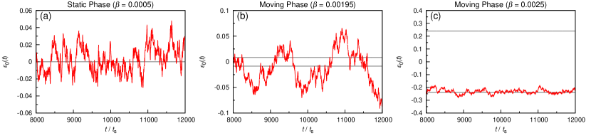
Figure F.1: (color online) Three samples of $\varepsilon_{0}\left(t\right)$ with dfferent values of $\tilde{\beta}$. (a) $\varepsilon_{0}\left(t\right)$ in the static phase. (b) $\varepsilon_{0}\left(t\right)$ in the moving phase near the static-moving transition. (c) $\varepsilon_{0}\left(t\right)$ in the moving phase. Parameters: $\tilde{k}=0.3$, $\tau_{{\rm d}}=50\tau_{{\rm s}}$ and $T=1\times 10^{-6}$.

Next, we consider the behavior in the moving phase. We start with the dynamical equations in the moving phase and in the presence of an external stimulus. We consider the case that the dynamics is dominated by a relaxation rate of the order $\lambda$, which is much slower than those of other distortion modes. For the example of SFA, we see that after the exposed profile couples with the inhibitory profile with a slow relaxation rate $\tau_{i}^{-1}$, there exists a family of inhibitory-like modes with relaxation rates approximately $\tau_{i}^{-1}$. Hence, we consider the regime $\lambda\ll\tau_{i}^{-1}$. (We conjecture that even when this condition is not satisfied, our analysis is still applicable because the inhibitory-like modes are weakly coupled with the external environment. We will leave this for further investigation.) This implies that the symmetric modes are effectively remaining at the instantaneous steady state. Hence interpreting the forces on the displacement modes as the couplings with the symmetric modes, we rewrite Eqs. (LABEL:eq:new_c0_tracking_2) and (119) as

$$-I_{u}v_{{\rm nat}}-M_{u1}v_{{\rm nat}}\varepsilon_{{\rm int}}^{2}-M_{u2}v_{{\rm nat}}^{2}\varepsilon_{{\rm int}}$$

$$\qquad=Q_{up}\varepsilon_{{\rm int}}+R_{u1}\varepsilon_{{\rm int}}^{3}+R_{u2}v_{{\rm nat}}\varepsilon_{{\rm int}}^{2}-I_{u}\eta,$$ (142)

$$-I_{p}v_{{\rm nat}}-M_{p1}v_{{\rm nat}}\varepsilon_{{\rm int}}^{2}-M_{p2}v_{{\rm nat}}^{2}\varepsilon_{{\rm int}}$$

$$\qquad=Q_{pp}\varepsilon_{{\rm int}}+R_{p1}\varepsilon_{{\rm int}}^{3}+R_{p2}v_{{\rm nat}}\varepsilon_{{\rm int}}^{2},$$ (143)

where $\eta$ is the positional noise defined in the main text. Considering the fluctuations around $v_{{\rm nat}}$ and $\varepsilon_{{\rm int}}$,

$$-I_{u}\delta v-M_{u1}\varepsilon_{{\rm int}}^{2}\delta v-2M_{u1}v_{{\rm nat}}\varepsilon_{{\rm int}}\delta\varepsilon_{0}$$

$$-M_{u2}v_{{\rm nat}}^{2}\delta\varepsilon_{0}-2M_{u2}v_{{\rm nat}}\varepsilon_{{\rm int}}\delta v$$

$$\qquad\qquad=Q_{up}\delta\varepsilon_{0}+3R_{u1}\varepsilon_{{\rm int}}^{2}\delta\varepsilon_{0}+R_{u2}\varepsilon_{{\rm int}}^{2}\delta v$$

$$\qquad\qquad\leavevmode\nobreak\ \leavevmode\nobreak\ \leavevmode\nobreak\ \leavevmode\nobreak\ +2R_{u2}v_{{\rm nat}}\varepsilon_{{\rm int}}\delta\varepsilon_{0}-I_{u}\eta,$$ (144)

$$I_{p}\frac{d}{dt}\delta\varepsilon_{0}-I_{p}\delta v-M_{p1}\varepsilon_{{\rm int}}^{2}\delta v-2M_{p1}v_{{\rm nat}}\varepsilon_{{\rm int}}\delta\varepsilon_{0}$$

$$-M_{p2}v_{{\rm nat}}^{2}\delta\varepsilon_{0}-2M_{p2}v_{{\rm nat}}\varepsilon_{{\rm int}}\delta v$$

$$\qquad\qquad=Q_{pp}\delta\varepsilon_{0}+3R_{p1}\varepsilon_{{\rm int}}^{2}\delta\varepsilon_{0}+R_{p2}\varepsilon_{{\rm int}}^{2}\delta v$$

$$\qquad\qquad\leavevmode\nobreak\ \leavevmode\nobreak\ \leavevmode\nobreak\ \leavevmode\nobreak\ +2R_{p2}v_{{\rm nat}}\varepsilon_{{\rm int}}\delta\varepsilon_{0}.$$ (145)

Eliminating $\delta v$,

$$\frac{d}{dt}\delta\varepsilon_{0}$$

$$= \leavevmode\nobreak\ \left(\frac{Q_{uu}}{I_{u}}+\frac{Q_{pp}}{I_{p}}\right)\delta\varepsilon_{0}-3\left(\frac{R_{u1}}{I_{u}}-\frac{R_{p1}}{I_{p}}\right)\varepsilon_{{\rm int}}^{2}\delta\varepsilon_{0}$$

$$-\left(\frac{R_{u2}+M_{u1}}{I_{u}}-\frac{R_{p2}+M_{p1}}{I_{p}}\right)\varepsilon_{{\rm int}}^{3}\delta v$$

$$-2\left(\frac{R_{u2}+M_{u1}}{I_{u}}-\frac{R_{p2}+M_{p1}}{I_{p}}\right)v_{{\rm nat}}\varepsilon_{{\rm int}}\delta\varepsilon_{0}$$

$$-2\left(\frac{M_{u2}}{I_{u}}-\frac{M_{p2}}{I_{p}}\right)v_{{\rm nat}}\varepsilon_{{\rm int}}\delta v$$

$$-\left(\frac{M_{u2}}{I_{u}}-\frac{M_{p2}}{I_{p}}\right)v_{{\rm nat}}^{2}\delta\varepsilon_{0}+\eta$$

$$= \leavevmode\nobreak\ \lambda\delta\varepsilon_{0}-3K_{1}\varepsilon_{{\rm int}}^{2}\delta\varepsilon_{0}-K_{2}\varepsilon_{{\rm int}}^{2}\delta v-K_{2}v_{{\rm nat}}\varepsilon_{{\rm int}}\delta\varepsilon_{0}$$

$$-K_{4}v_{{\rm nat}}\varepsilon_{{\rm int}}\delta v-K_{4}v_{{\rm nat}}^{2}\delta\varepsilon_{0}+\eta$$

Using Eq. (128) to eliminate $\lambda$, and $\delta\varepsilon_{0}=\tau_{{\rm int}}\delta v$,

$$\frac{d}{dt}\delta\varepsilon_{0}=-2\lambda\delta\varepsilon_{0}+\eta.$$ (147)

Solving the differential equation,

$$\delta\varepsilon_{0}\left(t\right)=\int_{-\infty}^{t}dt^{\prime}\exp\left[-2\lambda\left(t-t^{\prime}\right)\right]\eta\left(t\right).$$ (148)

Fluctuations are given by

$$\left\langle\delta\varepsilon_{0}\left(t\right)^{2}\right\rangle$$

$$= \leavevmode\nobreak\ \int_{-\infty}^{t}dt_{2}\int_{-\infty}^{t}dt_{1}e^{-2\lambda\left(t-t_{1}\right)-2\lambda\left(t-t_{2}\right)}\left\langle\eta\left(t_{1}\right)\eta\left(t_{2}\right)\right\rangle$$ (149)

$$= \leavevmode\nobreak\ \frac{T}{2\lambda}.$$ (150)

Connecting with the fluctuations with the response behavior through Eq. (131),

$$\frac{\left\langle\delta\varepsilon_{0}\left(t\right)^{2}\right\rangle}{T} =\frac{\tau_{{\rm stim}}\tau_{{\rm int}}}{2\left(\tau_{{\rm ant}}-\tau_{{\rm con}}\right)}\left(\frac{v_{{\rm nat}}^{2}-v_{I}^{2}}{v_{{\rm nat}}^{2}}\right)$$

$$\xrightarrow{\left|v_{{\rm nat}}\right|\gg\left|v_{I}\right|}\frac{\tau_{{\rm stim}}\tau_{{\rm int}}}{2\left(\tau_{{\rm ant}}-\tau_{{\rm con}}\right)}$$ (151)

Appendix F Numerical Measurement of $\left\langle\delta\varepsilon_{0}^{2}\right\rangle$

The variance of $\varepsilon_{0}\left(t\right)$ can be easily obtained from simulations, if the set of parameters is chosen to be far from phase boundaries. Those examples for CANNs with STD are shown in Fig. F.1 (a) and (c). In Fig. F.1(a), $\tilde{\beta}$ is small enough to have a stable static fixed point solution. In this case, there is only one fixed point solution of $\varepsilon_{0}=0$. The statistics of $\varepsilon_{0}\left(t\right)$ is relatively simple. For a large enough $\tilde{\beta}$, as shown in Fig. F.1(c), the two fixed point solutions to $\varepsilon_{0}$ have opposite signs and are separated far apart. As a result, $\varepsilon_{0}\left(t\right)$ will mostly stick to one of the fixed point solution. The statistics of $\varepsilon_{0}\left(t\right)$ is similar to that of the static phase.

However, in the moving phase near the phase boundary, e.g. Fig. F.1(b), the statistics may be problematic. The problem is due to the difference between two fixed point solutions being too small, so that $\varepsilon_{0}\left(t\right)$ is fluctuating around two fixed point solutions ($\varepsilon_{0,{\rm fixed}}^{+}$ and $\varepsilon_{0,{\rm fixed}}^{-}$), even though the noise temperature $T$ is small. Whenever $\varepsilon_{0}\left(t\right)$ is between two fixed point solutions, attractions due to fixed point solutions can affect our estimations of the variance of $\varepsilon_{0}\left(t\right)$ around a single fixed point solution.

To overcome the interference between two fixed point solutions, a trick is needed to filter out some data. In the statistics of Fig. 4 in the main text, we have discarded $\varepsilon_{0}\left(t\right)$ less than $\left|\varepsilon_{0,{\rm fixed}}^{+}\right|$. So, we approximate the variance by

$${\rm Var}\left[\varepsilon_{0}\left(t\right)-\varepsilon_{0,{\rm fixed}}^{\pm}\right]=\frac{\sum_{t^{\prime}\in S}\left[\left|\varepsilon_{0}\left(t^{\prime}\right)\right|-\left|\varepsilon_{0,{\rm fixed}}^{\pm}\right|\right]^{2}}{N_{{\rm sample}}-1},$$ (152)

where $S\equiv\left\{t^{\prime}\left|\left|\varepsilon_{0}\left(t^{\prime}\right)\right|>\left|\varepsilon_{0,{\rm fixed}}^{\pm}\right|\right.\right\}$ and $N_{{\rm sample}}\equiv\left|S\right|$.

References

- (1) A. Einstein, Ann. Phys. (Berlin) 322(8), 549 (1905).
- (2) M. von Smoluchowski, Ann. Phys. (Berlin) 326(14), 756 (1906).
- (3) H. Nyquist, Phys. Rev. 32, 110 (1928).
- (4) K. Huang, Statistical Mechanics (Wiley, New York, 1987).
- (5) R. Ben-Yishai, R. L. Bar-Or, and H. Sompolinsky, H. Proc. Natl. Acad. Sci. U.S.A. 92, 3844 (1995).
- (6) K. Zhang, The Journal of Neuroscience 16, 2112 (1996).
- (7) A. Samsonovich and B. L. McNaughton, J. Neurosci. 17, 5900 (1997).
- (8) H. Wilson and J. Cowan, Biophysical Journal12, 1 (1972).
- (9) S. Amari, S, Biological Cybernetics 27, 77 (1977).
- (10) R. Nijhawan and S. Wu, S. Phil. Trans. R. Soc. A 367, 1063 (2009).
- (11) J. O’Keefe and J. Dostrovsky, J. Brain Res. 34, 171 (1971).
- (12) J. S. Taube, R. U. Muller, and J. B. Ranck Jr., J. Neurosci. 10, 420 (1990).
- (13) J. S. Taube and R. I. Muller, Hippocampus 8, 87 (1998).
- (14) H. Y. Blair and P. E. Sharp, J. Neurosci. 15, 6260 (1995).
- (15) M. A. Sommer and R. H. Wurtz, Nature 444, 374 (2006).
- (16) R. Nijhawan, Nature (370), 256 (1994).
- (17) C. C. A. Fung, K. Y. M. Wong and S. Wu, Advances in Neural Information Processing Systems 25, 1097 (2013).
- (18) H. Wang, K. Lam, C. C. A. Fung, K. Y. M. Wong and S. Wu, arXiv:1502.03662 (2015).
- (19) R. Ben-Yshai, D. Hansel and H. Sompolinsky, J. Comp. Neurosci. 4, 57 (1997).
- (20) C. C. A. Fung and S. Amari, Neural Comput. 27, 507 (2015).
- (21) L. C. York and M. C. Van Rossum, J. Comput. Neurosci. 27, 607 (2009).
- (22) C. C. A. Fung, K. Y. M. Wong, H. Wang and S. Wu, Neural Comput. 24, 1147 (2012).
- (23) A., Treves, Network: Comput. in Neural Systems 4, 259 (1993).
- (24) W. Zhang and S. Wu, Neural Comput. 24, 1695 (2012).
- (25) S. Wu, K. Hamaguchi and S. Amari, Neural Comput. 20, 994 (2008).
- (26) C. C. A. Fung, K. Y. M. Wong and S. Wu, Neural Comput. 22, 752 (2010).
- (27) M. V. Tsodyks and H. Markram, Proc. Natl. Acad. Sci. U.S.A. 94, 719 (1997).
- (28) Y. Mi and C. C. A. Fung and K. Y. M. Wong and S. Wu, Adv. NIPS 27, 505 (2014).
- (29) S. Coombes and M. R. Owen, Phys. Rev. Lett. 94, 148102 (2005).
- (30) J. P. Goodridge and D. S. Touretzky, J. Neurophysio. 83, 3402 (2000).