To freeze or not to: Quantum correlations under local decoherence

Abstract

We provide necessary and sufficient conditions for freezing of quantum correlations as measured by quantum discord and quantum work deficit in the case of bipartite as well as multipartite states subjected to local noisy channels. We recognize that inhomogeneity of the magnetizations of the shared quantum states plays an important role in the freezing phenomena. We show that the frozen value of the quantum correlation and the time interval for freezing follow a complementarity relation. For states which do not exhibit “exact” freezing, but can be frozen “effectively”, by having a very slow decay rate with suitable tuning of the state parameters, we introduce an index – the freezing index – to quantify the goodness of freezing. We find that the freezing index can be used to detect quantum phase transitions and discuss the corresponding scaling behavior.

I Introduction

Characterizing correlations between different subsystems of a composite quantum system has been an important field of research in quantum information hhhh ; modi_rmp_2012 . This is due to the fact that quantum correlations, in the form of entanglement, is shown to be significantly more useful for performing communication and computational tasks over their classical counterparts ref1 . Moreover, these tasks have successfully been realized in the laboratory in several physical systems and thereby attracted a lot of attention in the field of detection and quantification of quantum correlations  exp . On the other hand, several non-intuitive results like local indistinguishability of orthogonal product states, non-classical efficiencies of a computational task by states having negligible entanglement, etc. have also been discovered ref2 ; ref3 ; dqci_group , which highlights the needs for conceptualization of quantumness in a composite system that is different from entanglement. This led to the introduction of quantum correlations like quantum discord (QD) disc_group and quantum work deficit (QWD) wdef_group that are independent of the entanglement paradigm.

One of the difficulties encountered in realizations of quntum information protocols is that quantum correlations decohere rapidly by interaction with the environment decohere_rev . Specifically, the intra-system quantum correlations decrease with time while the quantum correlations between the system and the environment increase. As a result, the system typically becomes less efficient in performing quantum information processing tasks. Therefore, the decay of quantum correlations with time in an open quantum system is a cause for concern. Consequently, knowledge of the behavior of quantum correlations in various quantum systems when subjected to different environments seems indispensable. Recent studies show that for a specific class of states, entanglement undergoes a sudden death sd_group ; sd_group2 ; sd_group3 at a finite time whereas QD decays asymptotically with time disc_dyn_group ; disc_dyn_group2 ; disc_dyn_group3 ; mazzola_prl_2010 ; adesso_pra_2013 ; disc_freez_group ; disc_expt_group .

Although a few studies have addressed the issue of preserving quantum correlation measures during their dynamics mazzola_prl_2010 ; adesso_pra_2013 ; disc_freez_group ; disc_expt_group , identifying the inherent property in quantum states, prohibiting the loss of quantum correlations over time, is still an open question. In the present work, we derive necessary and sufficient conditions for freezing of quantum correlation measures, for both QD and QWD, when a two-qubit state with magnetization is subjected to local depolarizing channels, in which bit-flip (BF), phase-flip (PF), or bit-phase-flip (BPF) errors can occur. We show that inhomogeneity in magnetization plays a crucial role for the freezing behavior of the state. The necessary and sufficient criteria show that there exist regions in which QD freezes while QWD does not, highlighting the necessity of proper choice of the quantum correlation measure to demonstrate the freezing phenomenon, and also that if the efficient performance of a certain quantum information task requires the freezing of a particular quantum correlation measure, the same may not remain efficient in a situation or environment where another quantum correlation is frozen. For both QD and QWD, we propose a complementarity relation between the quantum correlation during the freezing interval and the duration of the interval. For the class of states for which freezing is observed, we find a correspondence between the entanglement of the initial state and its freezing properties. The study is extended to multipartite states where two prescriptions for generating multipartite freezing states are proposed. Like decoherence-free subspaces decohere_free , introduced to protect qubits, the generated inherently decoherence-free states can be a building block of quantum memory q_mem in which quantum correlation in the form of QD or QWD can be stored.

Undoubtedly, the bipartite as well as the multipartite states which show freezing are of immense theoretical and experimental importance in quantum information processing tasks as they are inherently decoherence-free states for a finite time interval. However, there exists a large class of states for which quantum correlations do not freeze, but the change in quantum correlations is very slow with time. Hence it is interesting to quantify the freezing quality of a quantum correlation measure. We introduce a measure to quantify the goodness of freezing and call the measure as the “freezing index”. We then apply the measure to characterize the “effective freezing”of QD present in the anisotropic quantum $XY$ model in a transverse field xy_group , which appears in the description of certain solid-state realizations solid_xy , as well as in that of controlled laboratory settings num_trap_xy ; trap_rev ; lab_xy . Moreover, the index is capable of detecting the quantum phase transition in the model. The corresponding finite size scaling analysis has also been carried out.

The paper is organized as follows. In Section II, we briefly discuss the measures of quantum correlations used in this study and describe the methodology for investigating their dynamics in the presence of local noise. In Section III, the necessary and sufficient conditions for freezing of quantum correlations for bipartite states are derived and a complementarity of the value of the frozen quantum correlation with the freezing interval is obtained. The possible correspondence of the entanglement properties of the initial states to their freezing behavior is also addressed. Section IV deals with the generalization of the bipartite freezing behavior into multipartite cases. We discuss the phenomenon of effective freezing in Section V. There, we also quantify the quality of freezing by proposing a freezing index, and demonstrate its behavior in the case of the well-known transverse-field anisotropic $XY$ model. Section VI contains the concluding remarks.

II Quantum correlations: Definitions and dynamics

In this section, we provide a brief description of the quantum correlation measures used in the paper, namely, the QD and the QWD. We also present the methodology for investigating the dynamics of quantum correlations, when quantum states are subjected to local noise, and discuss the freezing of quantum correlations.

II.1 Quantum discord

In classical information theory, mutual information between two random variables $A$ and $B$ is defined as

$$I(A:B) = H(A)+H(B)-H(A,B)$$ (1)

$$= H(B)-H(B|A),$$

where $H(A)=-\sum_{i}p_{i}^{A}\log_{2}p_{i}^{A}$ is the Shannon entropy of $A$, and similarly for $H(B)$, while $H(A,B)$ is the joint entropy of $A$ and $B$. Here $H(B|A)=H(A,B)-H(A)$ is the conditional entropy of $B$ given $A$. Translation of these definitions into the quantum regime of bipartite quantum states leads to two inequivalent definitions of mutual information. One of them, which may be identified as the “total correlation”  of a bipartite quantum system $\rho_{AB}$, can be defined as tot_corr_group

$$I=S\left(\rho_{A}\right)+S\left(\rho_{B}\right)-S\left(\rho_{AB}\right),$$ (2)

where $\rho_{A}$ and $\rho_{B}$ are the states of the subsystems $A$ and $B$ respectively and $S\left(\rho\right)=-\mbox{Tr}\left[\rho\log_{2}\rho\right]$ is the von Neumann entropy of the quantum state $\rho$. An alternative definition of mutual information in the quantum regime takes the form disc_group

$$J_{\rightarrow}=S\left(\rho_{B}\right)-S\left(\rho_{B}|\rho_{A}\right),$$ (3)

where the sign ‘$\rightarrow$’ indicates that the measurement is being performed at $A$. Here $S(\rho_{B}|\rho_{A})=\sum_{k}p_{k}S\left(\rho_{AB}^{k}\right)$ is the measured quantum conditional entropy, where

$$\rho_{AB}^{k}=\left(\Pi_{k}^{A}\otimes I_{B}\right)\rho_{AB}\left(\Pi_{k}^{A}\otimes I_{B}\right)/p_{k}$$ (4)

and

$$p_{k}=\mbox{Tr}\left[\left(\Pi_{k}^{A}\otimes I_{B}\right)\rho_{AB}\right],$$ (5)

with $\{\Pi_{k}^{A}\}$ being a complete set of rank-$1$ projective measurement and $I_{B}$ denotes the identity operator on the Hilbert space of $B$. If $\rho_{A}$ is a single-qubit state, the rank-$1$ projectors are of the form $\Pi_{k}^{A}=|\Phi_{k}\rangle\langle\Phi_{k}|$, $k=1,2$, where

$$|\Phi_{1}\rangle = \cos\frac{\theta}{2}|0\rangle+e^{i\phi}\sin\frac{\theta}{2}|1\rangle$$

$$|\Phi_{2}\rangle = -e^{-i\phi}\sin\frac{\theta}{2}|0\rangle+\cos\frac{\theta}{2}|1\rangle,$$ (6)

with $0\leq\theta\leq\pi$ and $0\leq\phi<2\pi$, and with $\{|0\rangle,|1\rangle\}$ forming the computational basis of the qubit Hilbert space. The classical correlation (CC), $C_{\rightarrow}$, in the state $\rho_{AB}$, between the subsystems $A$ and $B$ can be quantified by maximizing $J_{\rightarrow}$ with respect to $\{\Pi_{k}^{A}\}$ disc_group , and is given by

$$C_{\rightarrow} = S\left(\rho_{B}\right)-\underset{\left\{\Pi_{A}^{k}\right\}}{\min}\sum_{k}p_{k}S\left(\rho_{AB}^{k}\right).$$ (7)

The difference between the total correlations and the CC provides the measure of quantum correlation, QD, and is given by

$$D_{\rightarrow} = S\left(\rho_{A}\right)-S\left(\rho_{AB}\right)+\underset{\left\{\Pi_{k}^{A}\right\}}{\min}\sum_{k}p_{k}S\left(\rho_{AB}^{k}\right).$$ (8)

There is an inherent asymmetry in the definition of the QD which implies that the value of the QD is not invariant with respect to the swapping of the parties. Throughout the paper, we denote the CC and the QD by $C$ and $D$ respectively, and calculate QD by performing the measurement on $A$. The optimization involved in the definition makes the analytical calculation of the QD, for an arbitrary bipartite state, a hard problem. However, for states with certain symmetries, such as the Bell-diagonal (BD) states, the optimization is known exactly luo_pra_2008 .

II.2 Quantum work deficit

The other information-theoretic quantum correlation measure that we consider is the QWD wdef_group . It is quantified as the difference between the amount of pure states extractable under suitably restricted global and local operations. For a bipartite state $\rho_{AB}$, we consider the class of global operations, termed “closed operations”  (CO), consisting of (i) unitary operations, and (ii) dephasing the bipartite state by a set of projectors, $\{\Pi_{k}\}$, defined on the Hilbert space $\mathcal{H}$ of $\rho_{AB}$. One can show that the amount of pure states extractable from $\rho_{AB}$ under CO is given by

$$I_{\mbox{\scriptsize CO\normalsize}}=\log_{2}\mbox{dim}\left(\mathcal{H}\right)-S(\rho_{AB}).$$ (9)

On the other hand, the class of “closed local operations and classical communication”  (CLOCC) consists of (i) local unitary operations, (ii) dephasing by local measurement on the subsystem $A$, and (iii) communicating the dephased subsystem to the other party, $B$, over a noiseless quantum channel. The average quantum state after the projective measurement $\{\Pi_{k}^{A}\}$ on $A$ is $\rho_{AB}^{\prime}=\sum_{k}p_{k}\rho_{AB}^{k}$ where $\rho_{AB}^{k}$ and $p_{k}$ are given by Eqs. (4) and (5), respectively. The amount of pure states extractable under CLOCC is given by

$$I_{\mbox{\scriptsize CLOCC\normalsize}}=\log_{2}\mbox{dim}\left(\mathcal{H}\right)-\underset{\left\{\Pi_{k}^{A}\right\}}{\min}S\left(\rho_{AB}^{\prime}\right).$$ (10)

The (one-way) QWD, $W$, is then defined as $W=I_{\mbox{\scriptsize CO\normalsize}}\left(\rho_{AB}\right)-I_{\mbox{\scriptsize CLOCC\normalsize}}\left(\rho_{AB}\right)$.

II.3 Local dynamics of quantum correlations

We will consider the situation where each qubit of a multi-qubit system interacts with an independent reservoir via decoherence channels. Following the Kraus operator formalism, the density matrix of a system of $N$ qubits, $\rho_{0}$, evolves with time as

$$\rho=\sum_{k_{1},\cdots,k_{N}}\tau_{k_{1}}^{(1)}\otimes\cdots\otimes\tau_{k_{N}}^{(N)}\rho_{0}{\tau_{k_{1}}^{(1)}}^{\dagger}\otimes\cdots\otimes{\tau_{k_{N}}^{(N)}}^{\dagger},$$

(11)

where $\{\tau_{k_{\alpha}}^{(\alpha)}\}$ describes the noisy channel acting on the qubit $\alpha$. The quantum channels describing the interaction of a qubit and its environment (the reservoir) can be of various types. We focus on three types of decoherence channels, namely, the bit-flip (BF), the phase-flip (PF), and the bit-phase-flip (BPF) channels. The Kraus operators for these channels are given by

$$\tau_{0}=\sqrt{1-\frac{\gamma}{2}}I_{2},\;\tau_{1}^{i}=\sqrt{\frac{\gamma}{2}}\sigma^{i},$$ (12)

where $\sigma^{i},\,i=1,\,2,\,3$, are the Pauli spin matrices and $I_{2}$ is the identity operator on the qubit Hilbert space. Here $\tau_{1}^{i}$, for $i=1,2$, and $3$ correspond to the BF, BPF and PF channels respectively. The decoherence probability, $\gamma$, called parametrized time, depends explicitly on time $t$ and is taken to be the same for all the qubits with $0\leq\gamma\leq 1$. It is convenient to describe the dynamical evolution of systems under decoherence channels in terms of the decoherence probabilities, since such description takes into account a wide range of physical situations. A particularly important class of physical scenarios is the one for which the functional dependence of the decoherence probability on time, $t$, describes the Markovian approximation, where $\gamma$ is often an increasing function, $f_{\Gamma}(t)$, of $t$, such as $\gamma=1-e^{-\Gamma t}$, with $\Gamma$ being a “decay rate”of the function yu_prl_2006 . When a non-Markovian environment is considered, $\gamma$ may be an oscillatory function of time with a decaying amplitude. One should note that under Markovian approximation, $\Gamma\neq 0$ and is fixed for a given bunch of local environments, with the corresponding evolution being scanned by varying $\gamma$. Once the time evolved density matrix, $\rho^{(\gamma)}$, is known, one can calculate its different quantum correlations as functions of system parameters and the decoherence probability, to investigate their dynamical behavior under various decoherence channels.

II.4 Freezing

Even as quantum correlations continue to be regarded as fragile quantities, there are undespairing efforts to control such decay. An interesting possibility is the identification of shared quantum states that offer a stagnant or near-constant behavior of quantum correlations when affected by noisy time-dynamics. In case we find that a quantum correlation measure is a constant in time for a certain time interval, we say that it is exhibiting the phenomena of freezing.

III Freezing in two-qubit systems

A general two-qubit state can be written, up to local unitary transformations luo_pra_2008 ; fano_rmp_1983 , as

$$\rho_{AB} = \frac{1}{4}[I_{A}\otimes I_{B}+\sum_{\alpha=1}^{3}c_{\alpha\alpha}\sigma_{A}^{\alpha}\otimes\sigma_{B}^{\alpha}$$ (13)

$$+\sum_{\alpha=1}^{3}c_{\alpha 0}\sigma_{A}^{\alpha}\otimes I_{B}+\sum_{\beta=1}^{3}c_{0\beta}I_{A}\otimes\sigma_{B}^{\beta}],$$

where the diagonal correlators, $c_{\alpha\alpha}=\mbox{Tr}[\sigma^{\alpha}\otimes\sigma^{\alpha}\rho_{AB}]$, represent “classical”  correlators, the single-qubit quantities, $c_{\alpha 0}=\mbox{Tr}[\sigma^{\alpha}\otimes I_{B}\rho_{AB}]$ and $c_{0\beta}=\mbox{Tr}[I_{A}\otimes\sigma^{\beta}\rho_{AB}]$, are the magnetizations, and $I_{A}$ and $I_{B}$ are identity operators on the Hilbert spaces of $A$ and $B$ respectively.

To address the question of freezing of quantum correlations in bipartite states under local noise, we first focus our attention on the BF channel. Using Eq. (11), it is easy to show that during the BF evolution of $\rho_{AB}$, $c_{11}$, $c_{10}$, and $c_{01}$ remain unchanged, whereas the correlators $c_{\alpha\alpha}$ and the magnetizations $c_{0\alpha}$ and $c_{\alpha 0}$ ($\alpha=2,3$) decay with $\gamma$ as $(1-\gamma)^{2}$ and $(1-\gamma)$ respectively. To observe freezing phenomena of quantum correlation measures under the BF channel, it is therefore reasonable to choose the bipartite state of the form

$$\rho_{AB} = \frac{1}{4}[I_{A}\otimes I_{B}+\sum_{\alpha=1}^{3}c_{\alpha\alpha}\sigma_{A}^{\alpha}\otimes\sigma_{B}^{\alpha}$$ (14)

$$+\left(c_{10}\sigma_{A}^{1}\otimes I_{B}+c_{01}I_{A}\otimes\sigma_{B}^{1}\right)],$$

with $c_{\alpha\alpha}\neq 0$ as the initial state of the quantum evolution. We refer to these states as the canonical initial states. Next, we will show that to preserve quantum correlation from decohering, inhomogeneous magnetizations play an important role. The analysis is henceforth mainly carried out for the local BF channel. However, a straightforward generalization of the presented results is possible for other local quantum channels, in particular, the PF and the BPF channels.

III.1 Freezing of QD

We begin by investigating the freezing dynamics of quantum correlations, as measured by the QD, using the canonical initial states. Unlike the Bell-diagonal (BD) states luo_pra_2008 , QD of the states evolved from CI states cannot be computed analytically num-err_group . However, numerical simulations show that for a large fraction of states – special CI (SCI) states $(\mathcal{S}_{1})$ – the optimization takes place for the projectors corresponding to three sets of “regular”  values $\{\theta,\phi\}$: $s_{1}=\{\theta=0,\pi\}$, $s_{2}=\{\theta=\pi/2,\phi=\pi/2,3\pi/2\}$, and $s_{3}=\{\theta=\pi/2,\phi=0,\pi\}$. The existence of the complementary class, which we denote by $\mathcal{S}_{2}$, makes the analytical calculation of the QD for $\rho_{AB}$ difficult. If $D$ denotes the QD of the state $\rho_{AB}$ and $D^{\prime}$ represents the QD calculated with the assumption that $\rho_{AB}\in\mathcal{S}_{1}$, then our numerical analysis shows that $\epsilon<0.0028$, where $\epsilon=\max\{D^{\prime}-D\}$ is the maximum value of the error due to the assumption. Similar findings have been reported earlier for two-qubit $X$ states num-err_group . For the numerical simulation, the two-qubit canonical initial state, $\rho_{AB}$, is generated on a grid with a separation of $\sim 10^{-3}$ for all correlators, $c_{\alpha\alpha}$, and magnetizations, $c_{10}$ and $c_{01}$. Proposition I provide a necessary and sufficient criterion for freezing of QD for the SCI states. Numerical evidence strongly suggests that the proposition holds for the entire class of CI states up to the second decimal place.

Proposition I. If a two-qubit SCI state is sent through local BF channels, an NS condition for the QD in the evolved state to remain constant over a finite interval of time is given by either of the following sets of equations:

$$\begin{cases}(i)&(c_{22}/c_{33})=-(c_{10}/c_{01})=-c_{11},\\ (ii)&c_{33}^{2}+c_{01}^{2}\leq 1,\\ (iii)&F\left(\sqrt{c_{33}^{2}+c_{01}^{2}}\right)\leq F(c_{11})+F(c_{01})-F(c_{10});\end{cases}$$

(15)

$$\begin{cases}(i)&(c_{33}/c_{22})=-(c_{10}/c_{01})=-c_{11},\\ (ii)&c_{22}^{2}+c_{01}^{2}\leq 1,\\ (iii)&F\left(\sqrt{c_{22}^{2}+c_{01}^{2}}\right)\leq F(c_{11})+F(c_{01})-F(c_{10}).\end{cases}$$

(16)

Here, $F(y)=2\left(H(\frac{1+y}{2})-1\right)$, with $H(\alpha)=-\alpha\log_{2}\alpha-(1-\alpha)\log_{2}(1-\alpha)$ being the binary entropy function.

Note: We call the function $F$ as the “freezing entropy”  and the relations (15)(iii) and (16)(iii) as the “freezing subadditivity”  I and II, for the QD, respectively.

Proof. For a state $\rho_{AB}\in\mathcal{S}_{1}$, QD is given by $D=\min\{D_{l}\}$ where $l=1,2,$ and $3$ correspond to the sets $s_{1}$, $s_{2}$, and $s_{3}$, respectively, with

$$D_{l} = S(\rho_{A})-S(\rho_{AB}^{(\gamma)})-\sum_{i}p_{i}\sum_{ij}\chi_{ij}\log_{2}\chi_{ij}\delta_{l3}$$ (17)

$$+(1-\delta_{l3})(1+F(c^{\prime}_{\delta})/2).$$

Here, $\delta_{ll{{}^{\prime}}}$ denote the Kronecker delta, ${c^{\prime}_{\delta}}^{2}=c_{01}^{2}+(1-\gamma)^{4}(c_{33}^{2}\delta_{l1}+c_{22}^{2}\delta_{l2})$, $p_{i}=\frac{1}{2}\left(1+(-1)^{i}c_{10}\right)$, and $\chi_{ij}=(1+(-1)^{i}c_{10}+(-1)^{j}(c_{01}+(-1)^{i}c_{11}))/2\left(1+(-1)^{i}c_{10}\right)$. Note that the marginal states $\rho_{A}$ and $\rho_{B}$ of the canonical initial state $\rho_{AB}$ do not vary with $\gamma$. Let us first focus on the necessity of the conditions given in (15) and (16). If freezing of QD takes place, $D$ must be invariant with $\gamma$ for a finite interval. Let us assume that $D=D_{1}$, in that interval. From the expression of $D_{1}$, it is easy to show that for $D_{1}$ to be independent of $\gamma$, condition (15)(i) must be satisfied. Under this condition, (15)(ii) is required to ensure the positivity of the initial state $\rho_{AB}\in\mathcal{S}_{1}$. Since $D_{1}=\min\{D_{l}\}$, $l=1,2,3$, $D_{3}$ must be greater that $D_{1}$ which leads to the condition (15)(iii), thereby proving the necessity of the group of conditions given in (15) for the occurrence of freezing of QD. Next, we assume that $D=D_{2}$. In a similar fashion as in the previous case, one can show that the set of conditions given in (16) is necessary for the freezing of QD. Lastly, let $D=D_{3}$. From Eq. (17), it is easy to see that the only term dependent on $\gamma$ is $S(\rho_{AB}^{(\gamma)})$. The eigenvalues of the time evolved state $\rho_{AB}^{(\gamma)}$ with the state $\rho_{AB}\in\mathcal{S}_{1}$ as the initial state can be easily determined to be

$$\lambda_{1} = \frac{1}{4}(1+c_{11}-\sqrt{(c_{10}+c_{01})^{2}+(\gamma-1)^{4}(c_{22}-c_{33})^{2}}),$$

$$\lambda_{2} = \frac{1}{4}(1+c_{11}+\sqrt{(c_{10}+c_{01})^{2}+(\gamma-1)^{4}(c_{22}-c_{33})^{2}}),$$

$$\lambda_{3} = \frac{1}{4}(1-c_{11}-\sqrt{(c_{10}-c_{01})^{2}+(\gamma-1)^{4}(c_{22}+c_{33})^{2}}),$$

$$\lambda_{4} = \frac{1}{4}(1-c_{11}+\sqrt{(c_{10}-c_{01})^{2}+(\gamma-1)^{4}(c_{22}+c_{33})^{2}}).$$

(18)

One can easily show that $S(\rho_{AB}^{(\gamma)})$ varies with $\gamma$ for all possible non-zero values of the correlators and the magnetizations which is not possible if QD freezes. Hence (15) and (16) are the necessary conditions for the occurrence of freezing in QD in the case of initial two-qubit states $\rho_{AB}\in\mathcal{S}_{1}$.

To prove the sufficiency of the conditions, we first consider the set of conditions in (15). If condition (15)(i) is imposed over the initial two-qubit state $\rho_{AB}\in\mathcal{S}_{1}$, it can be shown that $D_{1}$ is independent of time for all values of $\gamma$. One should note that a condition similar to this one has earlier been reported for the PF channel li_pra_2011 . For $\left|c_{11}\right|=1$, the initial state is a pure state with QD monotonically decaying with $\gamma$. Moreover, $D_{2}>D_{1}$ $\forall$ $\gamma$, when Eq. (15)(i) is satisfied implying that the QD is given by $D=\min\{D_{l}\}$ with $l=1,3$. Besides (15)(i), condition (15)(ii) ensures positivity of the initial two-qubit state $\rho_{AB}\in\mathcal{S}_{1}$. Application of conditions (15)(i)-(ii) leads to the following forms of the functions $D_{1}$ and $D_{3}$:

$$D_{1} = \frac{1}{2}(F(c_{10})-F(c_{11})),$$

$$D_{3} = \frac{1}{2}(F(c_{01})-F(c^{\prime})).$$ (19)

Here, ${c^{\prime}}^{2}=c_{01}^{2}+c_{33}^{2}(1-\gamma)^{4}$. Note that $D_{3}$ is a monotonically decreasing function of $\gamma$. When condition (15)(iii) is applied, we get $D_{3}>D_{1}$ for a finite interval of time in which QD freezes. Similarly, one can prove that the QD, given by $D_{2}$, is invariant with $\gamma$ when the sets of conditions given in (16) are obeyed. Hence for the two-qubit states $\rho_{AB}\in\mathcal{S}_{1}$, the set of conditions (15) and (16) are both necessary and sufficient for the QD to remain constant under the BF noise. $\blacksquare$

The freezing phase diagram on the $(c_{33},c_{01})$ plane, for SCI states, is exhibited in Fig. 1(a) for a fixed value of $|c_{11}|=0.6$. For given values of $c_{11}$, one obtains different freezing phase diagrams depending on whether condition (15) or (16) is used. Here we chose condition (15) for Fig. 1(a). Then, the states that show freezing of QD under the BF channel are enclosed by the circle $c_{01}^{2}+c_{33}^{2}=1$ and also satisfy the freezing subadditivity I for QD. The white region outside the circle depicts states that violate positivity. Freezing occurs, for a finite parametrized time interval , $0\leq\gamma\leq\gamma_{f}$, within the two crescents – they form the “freezing crescents”  for QD for the chosen parameter space. We refer to $\gamma_{f}$ as the “freezing terminal”. The freezing crescents as well as the freezing terminals are functions of the input quantum state, the channel, and the measure employed to quantify quantum correlations. $\gamma_{f}$ can be found by solving

$$F(\sqrt{c_{01}^{2}+c_{33}^{2}(1-\gamma)^{4}})=F(c_{11})+F(c_{01})-F(c_{10}).$$ (20)

In Fig. 1(a), the $\gamma_{f}$ are mapped onto the freezing crescents in the phase diagram. The states for which freezing takes place are indicated by the faded regions while the black region represents states for which the QD decays with $\gamma$. The different shades in the freezing crescents indicate the values of the freezing terminal, $\gamma_{f}$. Note that the states inside the freezing crescents can be generated by BF evolution from the states lying on the perimeter of $c_{33}^{2}+c_{01}^{2}=1$. If $|c_{11}|$ is decreased, the freezing region expands, thereby indicating an increase in $\gamma_{f}$ for fixed $c_{33}$ and $c_{01}$, although the value of the frozen QD decreases. We revisit this issue in Proposition IV. Note that choosing condition (16) to draw the freezing phase diagram, the corresponding $\gamma_{f}$ would be given by the equation obtained by replacing $c_{33}$ by $c_{22}$ Eq. (20).

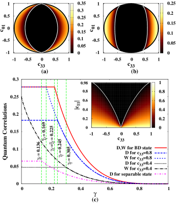
Figure 1: (Color online) Freezing phase diagram. The freezing of (a) QD and (b) QWD under local BF channels for the CI states with $|c_{11}|=0.6$ and obeying condition (a) (15)(i) for QD and (b) (24)(i) for QWD. See text for details. (c) The dynamics of quantum correlations, as measured by the QD and the QWD, using two-qubit CI states obeying conditions (15) or (24) with $c_{33}^{2}+c_{01}^{2}=1$. For all of these states, the value of $|c_{11}|=0.6$. Inset: Another freezing phase diagram for QWD on the $(c_{33},|c_{11}|)$ plane for the CI states obeying condition (24)(i)-(iii) with $c_{33}^{2}+c_{01}^{2}=1$. All quantities plotted are dimensionless, except QD, which is in bits, and QWD, which is in qubits.

Let us now state two corollaries which follow directly from Proposition I.

Corollary 1. When an SCI state, satisfying the NS freezing conditions for QD, is subjected to local BF noise, the freezing terminal attains its maximum value for given values of $c_{11}$ and $c_{01}$, at the maximum allowed value of $\left|c_{33}\right|$ or $\left|c_{22}\right|$.

Proof. From Eqs. (15) and (20), $c_{01}^{2}+c_{33}^{2}(1-\gamma_{f})^{4}=\textrm{constant}$ for fixed $c_{11}$ and $c_{01}$. This implies that $\gamma_{f}$ attains its maximum value for $|c_{33}|_{max}=\sqrt{1-c_{01}^{2}}$. A similar proof exists if Eq. (16) is considered instead of Eq. (15). $\blacksquare$

Corollary 2. When an SCI state is subjected to local BF noise, the QD will always decay if the magnetization is homogeneous.

Proof. Homogeneity of magnetization implies $c_{01}=c_{10}$, and from Eq. (15)(i) or (16)(i), it is clear that the homogeneity of non-zero magnetization requires $\left|c_{11}\right|=1$ which violates the necessary condition for freezing of QD in SCI states. $\blacksquare$

Note that if $c_{01}=c_{10}=0$, the CI state reduces to a BD state, in which freezing of different quantum correlations occur  mazzola_prl_2010 ; adesso_pra_2013 ; disc_freez_group ; disc_expt_group . In the case of the BD states, the second relation in (15)(i) (or in (16)(i)) does not hold while the first condition is still valid and gives a necessary condition for freezing mazzola_prl_2010 ; adesso_pra_2013 . In Fig. 1(a), for $c_{01}=0$, the BD states are along the horizontal diameter of the circle. The two end points of that diameter represent BD states for which QD is known to exhibit freezing mazzola_prl_2010 . The dynamics of QD for the BD state with $|c_{11}|=|c_{22}|=0.6$, $|c_{33}|=1$, $c_{01}=c_{10}=0$ is shown in Fig. 1(c). Note that there exist initial states, eg. the states satisfying (15) and lying on $c_{33}^{2}+c_{01}^{2}=1$, for which freezing terminals longer than that of the BD state can be achieved (Fig. 1(c)). Identifying such a state with a prolonged constancy of QD under decoherence can be of vital importance in realizing quantum information protocols.

The results mentioned above are only for the SCI states that satisfy conditions (15)(i)-(iii). Our numerical findings suggest that a small fraction of the states that obey conditions (15)(i) and (ii) belong to the set $\mathcal{S}_{2}$. Extensive numerical simulations indicate that such states are found only in the regions on the freezing phase diagram where the quantum states do not show freezing behavior. Irrespective of the optimal sets in the measurement of QD, Proposition I and numerical simulations strongly suggest that the QD of the entire class of CI states, would exhibit freezing if and only if they satisfy the conditions (15)(i) and (15)(ii).

III.2 Freezing of QWD

We now move on to investigate the freezing phenomena for other information-theoretic quantum correlation measures. Freezing of QD has been extensively studied for BD states, for which QWD and QD coincide wdef_group . Let us consider an arbitrary bipartite state, $\varrho_{AB}$, of which $\varrho_{A(B)}$ is the marginal state of the subsystem $A(B)$ obtained by tracing out the other subsystem $B(A)$, and advance to the following proposition.

Proposition II. For a given bipartite state $\varrho_{AB}$ evolving under local BF channels, if the optimizations in QD and QWD occur in the same optimal ensemble $\{\bar{p}_{k},\bar{\varrho}_{AB}^{k}\}$ for $\gamma\leq\gamma_{f}$, and if $H\left(\left\{\bar{p}_{k}\right\}\right)-S\left(\varrho_{A}\right)$ is independent of time for the same interval, then QWD freezes for $\gamma\leq\gamma_{f}$ provided QD freezes for $\gamma\leq\gamma_{f}^{0}$ where $\gamma_{f}^{0}\geq\gamma_{f}$.

Proof. From the definitions of QD and QWD, we get

$$W = D-S\left(\varrho_{A}\right)+\underset{\left\{\Pi_{A}^{k}\right\}}{\mbox{min}}\sum_{k}p_{k}S\left(\varrho_{AB}^{k}\right)$$ (21)

$$-\underset{\left\{\Pi_{A}^{k}\right\}}{\mbox{min}}S\left(\sum_{k}p_{k}\varrho_{AB}^{k}\right).$$

Using the concavity of von Neumann entropy,

$$\sum_{k}\bar{p}_{k}S\left(\bar{\varrho}_{AB}^{k}\right)=S\left(\sum_{k}\bar{p}_{k}\bar{\varrho}_{AB}^{k}\right)+H\left(\left\{\bar{p}_{k}\right\}\right),$$ (22)

using which, we reach

$$W=D-S\left(\varrho_{A}\right)+H\left(\left\{\bar{p}_{k}\right\}\right),$$ (23)

provided both the minimizations in Eq. (21) take place for the same ensemble. If Eq. (23) is satisfied, the freezing of QWD demands the freezing of QD, provided $H\left(\left\{\bar{p}_{k}\right\}\right)-S\left(\rho_{A}\right)$ is constant in time in the relevant interval. Note that the result is not restricted to two-qubit states. $\blacksquare$

For the SCI states, the conditions in the above proposition can be relaxed. Specifically, we obtain the following corollary.

Corollary 3. When an SCI state is sent through local BF channels, QWD freezes whenever QD shows freezing behavior, provided the optimizations occur for the same ensemble.

Proof. For an SCI state, $\rho_{AB}$, $S(\rho_{A})$ remains unaltered with time. From the relation between QD and QWD given in Eq. (23), for $\rho_{AB}$, we find that $\bar{p}_{k}=1/2$ $\forall k$ whenever QD freezes and hence the proof. $\blacksquare$

Similarly as for QD, numerical investigation shows that also in the case of QWD, there exist two sets of states, $\tilde{\mathcal{S}}_{1}$ and $\tilde{\mathcal{S}}_{2}$, depending on the optimal measurements. For the states $\rho_{AB}\in\tilde{\mathcal{S}}_{1}$, the optimization of QWD takes place for the projectors corresponding to three sets of “regular” values, while the rest of the states constitute the set $\tilde{\mathcal{S}}_{2}$. Interestingly, for the states $\rho_{AB}\in\tilde{\mathcal{S}}_{1}$, the three regular sets are identical to those for QD. We also observe that the set of states, for which the optimal measurements are at irregular values, is small. Let us now state the NS condition for the freezing behavior of QWD.

Proposition III. If a two-qubit state in $\tilde{\mathcal{S}}_{1}$ is sent through local BF channels, an NS condition for QWD in the evolved state to remain constant over a finite interval of time is given by either of the following sets of equations:

$$\begin{cases}(i)&\frac{c_{22}}{c_{33}}=-\frac{c_{10}}{c_{01}}=-c_{11},\\ (ii)&c_{33}^{2}+c_{01}^{2}\leq 1,\\ (iii)&F\left(\sqrt{c_{33}^{2}+c_{01}^{2}}\right)\leq F(c_{11})+F(c_{01}));\end{cases}$$

(24)

$$\begin{cases}(i)&\frac{c_{33}}{c_{22}}=-\frac{c_{10}}{c_{01}}=-c_{11},\\ (ii)&c_{22}^{2}+c_{01}^{2}\leq 1,\\ (iii)&F\left(\sqrt{c_{22}^{2}+c_{01}^{2}}\right)\leq F(c_{11})+F(c_{01})).\end{cases}$$

(25)

Proof. Proceeding in a similar fashion as in the case of QD, it can be shown that QWD of the time evolved two-qubit state, $\rho_{AB}^{(\gamma)}$, is given by $W=\min\{W_{l}\}$ with $l=1,2,$ and $3$ corresponding to the three sets of $\{\theta,\phi\}$ values, $s_{1}$, $s_{2},$ and $s_{3}$, where

$$W_{l} = 2(\delta_{l1}+\delta_{l2})-S(\rho_{AB}^{(\gamma)})-\delta_{l3}\sum_{i=1}^{4}\lambda_{i}\log_{2}\lambda_{i}$$ (26)

$$+\frac{1}{2}F\left(\sqrt{c_{01}^{2}+(c_{33}^{2}\delta_{l1}+c_{22}^{2}\delta_{l2})(1-\gamma)^{4}}\right).$$

Here,

$$\lambda_{1} = \frac{1}{4}\left(1+c_{01}+c_{10}+c_{11}\right),$$

$$\lambda_{2} = \frac{1}{4}\left(1-c_{01}-c_{10}+c_{11}\right),$$

$$\lambda_{3} = \frac{1}{4}\left(1-c_{01}+c_{10}-c_{11}\right),$$

$$\lambda_{4} = \frac{1}{4}\left(1+c_{01}-c_{10}-c_{11}\right).$$

We begin with the proof for the necessity of the conditions (24) and 25. First, let us assume that the QWD is given by $W_{1}$. For freezing to occur, $W_{1}$ must be independent of $\gamma$ in a finite interval. It is easy to show that if $W_{1}$ is independent of $\gamma$, then condition (24)(i) is satisfied. Then to ensure the positivity of the initial state, condition (24)(ii) must be satisfied. Also, $W=W_{1}$ implies that $W_{3}>W_{1}$ for a finite range of $\gamma$ leading to the condition (24)(iii). Hence the set of conditions (24) is necessary for freezing of QWD when $W=W_{1}$. In a similar fashion, one can show that the set of conditions (25)(i)-(iii) is necessary for freezing of QWD when $W=W_{2}$. For $W=W_{3}$, similar to the case of the QD, the $\gamma$-dependence comes through the term $S(\rho_{AB}^{(\gamma)})$ which can be determined using the eigenvalues given in Eq. (18). One can easily show that the function $W_{3}$ always depends on $\gamma$ for all possible values of the correlators and magnetizations, thereby proving that freezing of QWD is not possible for $W=W_{3}$. Hence the sets of conditions given in (24) and (25) are necessary for freezing to occur in the case of QWD with $\rho_{AB}\in\tilde{\mathcal{S}}_{1}$ as initial states.

To prove the sufficiency of the conditions, we start with the set of conditions (24). When condition (24)(i) is imposed, the function $W_{1}$ is independent of $\gamma$, and $W_{2}>W_{1}$, implying $W=\min\{W_{l}\}$ with $l=1,3$. The second condition of (24) is required to ensure positivity of the initial state once the condition (24)(i) is applied. Under the conditions (24)(i) and (ii), $W_{1}=-\frac{1}{2}F(c_{11})$ whereas $W_{3}=\frac{1}{2}(F(c_{01})-F(\sqrt{c_{01}^{2}+c_{33}^{2}(1-\gamma)^{4}}))$, which decreases monotonically with $\gamma$. If the third condition of (24) is applied, $W_{3}>W_{1}$ for a finite range of $\gamma$ so that $W=W_{1}$ in that range. Since $W_{1}$ is invariant with $\gamma$, freezing of QWD takes place in that range thereby proving the sufficiency of the set of conditions (24). Following a similar path, one can show that $W=W_{2}$ freezes for a finite interval of $\gamma$, when conditions (25) are applied. $\blacksquare$

Comparison. There are clear signatures that point to differences in the behavior of QD and QWD in the dynamics. In particular, extensive numerical searches show that no CI state satisfying (24)(i) and (ii) is in $\tilde{\mathcal{S}}_{2}$. This is in stark contrast to the findings for QD. Like QD, the freezing terminal, $\tilde{\gamma}_{f}$, for QWD can be determined as the solution of the equation $W_{1}=W_{3}$ (assuming conditions (24)). The freezing of the QWD is depicted in the $(c_{33},c_{01})$ plane in Fig. 1(b) for CI states with $|c_{11}|=0.6$ and when the conditions (24)(i) and (ii) are obeyed. For fixed parameters, the freezing region for QWD can be smaller than that of QD, indicating the existence $\rho_{AB}\in\mathcal{S}_{1}$ for which QD freezes but QWD does not. Interestingly, for such states, we find that the optimal projectors are different for QD and QWD. Eg., see Fig. 1(c) for $c_{33}=0.4$. The inset of Fig. 1(c) maps the $\gamma_{f}$ for the QWD in the $(|c_{11}|,c_{33})$ plane under condition (24) with $c_{01}^{2}+c_{33}^{2}=1$. The shades represent similar situations as in the case of Fig. 1(a). The black inner region between the two curves correspond to states for which the QWD decay monotonically under the BF noise and exhibit no freezing. Contrary to the behaviour of QWD, QD shows freezing for all states on the $(|c_{11}|,c_{33})$ plane under the same condition except at $c_{33}=0$, for which the initial state is completely classical. This is an example where the behavior of QD and QWD differ in a very drastic way. In contrast to earlier findings, focussing on BD states adesso_pra_2013 , our analysis clearly shows that freezing of quantum correlations depends explicitly on the choice of the correlation measures.

III.3 Complementarity

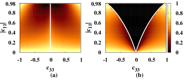
Figure 2: (Color online) Complementarity. Value of $Q_{f}+\gamma_{F}$ for QD (a) and QWD (b) using the canonical initial state obeying Eq. (15) and (24) respectively with $c_{33}^{2}+c_{01}^{2}=1$ as the initial state under BF dynamics. The sum $Q_{f}+\gamma_{F}$ is represented by different shades, as indicated by the color-bar, on the $(c_{33},|c_{11}|)$ plane. The QD is zero for $c_{33}=0$ (the white vertical line in (a)). For QWD, $\tilde{\gamma}_{f}=0$ above the white curves in (b), as shown earlier (inset of Fig. 1(c)). The dimensions are the same as in Fig. 1.

From the freezing behavior of QD and QWD, we observe that for the CI states, the frozen values of the quantum correlation measures increase while the freezing terminals decrease with the tuning of appropriate system parameters. This observation is made more precise in Proposition IV.

Proposition IV. If a two-qubit BD state freezes under local BF noise, the frozen quantum correlation $Q_{f}$, as measured by QD or QWD, and the freezing terminal, $\gamma_{F}$, satisfy the complementarity relation

$$Q_{f}+\gamma_{F}\leq 1,$$ (28)

where $\gamma_{F}=\gamma_{f}$ or $\tilde{\gamma}_{f}$, respectively.

Proof. In the case of the BD states, $c_{10}=c_{01}=0$ in Eq. (14), and the QD, under condition (15), is given by $D=-\frac{1}{2}F(c_{11})$, so that $\gamma_{f}=1-\sqrt{|c_{11}|/|c_{33}|}$. Now, $D+\gamma_{f}$ is an even function of $c_{11}$, having no maxima and a single minima between $0$ and $1$. As a function of $c_{33}$, $D+\gamma_{f}$ attains its maximum at $|c_{33}|=1$. The maximal value of the function is $1$ for $c_{11}=0,\pm 1$. Since $W=D$ in the case of the BD state, the proposition holds for QWD as well. $\blacksquare$

Now the question remains whether the complementary relation holds for other classes of states. For the CI states that obey condition (15), the values $\gamma_{f}$ are obtained by the implicit equation (20). Similar equations can be solved for the other cases. Numerical analysis with such equations reveal that the complementarity relation (28) is valid for all possible states satisfying the NS conditions in Proposition I and III, and therefore correspond to both QD and QWD. Specifically, we find that the maximum of $Q_{f}+\gamma_{F}$ is $1$, and occurs only when $c_{11}=0$ or $|c_{11}|=|c_{33}|=1$ (see Fig. 2).

III.4 Non-convexity

Up to now, we have concentrated on the conditions on the parameters of the class of states for which QD and QWD freeze. We now study the properties of the set of states which show freezing for QD as well as those for QWD. In particular, we have the following proposition.

Proposition V. The SCI states that exhibit freezing of QD form a non-convex set. The same is true for QWD.

Proof. If the sets are convex, then the state $\rho=p\rho^{1}_{AB}+(1-p)\rho^{2}_{AB}$ for all $0\leq p\leq 1$ will be a state that will exhibit freezing, if $\rho^{1}_{AB}$ and $\rho^{2}_{AB}$ does so. We note that the necessary conditions for freezing for both the QD and the QWD are given in (15)(i) and (16)(ii). Therefore, for convexity to hold, we must have the relation

$$\frac{pc_{22}^{1}+(1-p)c_{22}^{2}}{pc_{33}^{1}+(1-p)c_{33}^{2}} = -\frac{pc_{10}^{1}+(1-p)c_{10}^{2}}{pc_{01}^{1}+(1-p)c_{01}^{2}}$$ (29)

$$= -pc_{11}^{1}-(1-p)c_{11}^{2},$$

or the relation

$$\frac{pc_{33}^{1}+(1-p)c_{33}^{2}}{pc_{22}^{1}+(1-p)c_{22}^{2}} = -\frac{pc_{10}^{1}+(1-p)c_{10}^{2}}{pc_{01}^{1}+(1-p)c_{01}^{2}}$$ (30)

$$= -pc_{11}^{1}-(1-p)c_{11}^{2}.$$

true for all $p$. Here, $c_{\alpha\alpha}^{1}$ and $c_{\alpha\alpha}^{2}$, $\alpha=0,1,2,3$ denote the correlators and magnetizations of $\rho_{AB}^{1}$ and $\rho_{AB}^{2}$ respectively. For arbitrary values of the correlators, the above equations are not satisfied except for $p=0,1,$ proving the non-convexity of the sets. $\blacksquare$

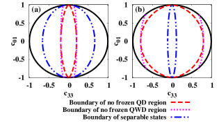
Figure 3: (Color online) The boundaries of the entangled and freezing regions for QD and QWD are plotted for $|c_{11}|=0.2$ (a) and $|c_{11}|=0.8$ (b). Clearly, the entangled region increases as the value of $|c_{11}|$ increases, while the trend is opposite for the freezing regions of QD and QWD. All quantities plotted are dimensionless.

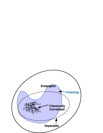
Figure 4: (Color online) States having non-zero quantum correlation that exhibit freezing under local noise are in the shaded region. While the separable states contain the classically correlated states, the freezing states do not, and while the class of separable states is convex, the others are not.

III.5 Relation between entanglement and freezing

We have already found the conditions by which QD and QWD of two-qubit mixed states remain constant with time in the presence of local noise. On the other hand, entanglement of the state undergoes sudden death when local BF channels are applied sd_group . However, we find that the behavior of entanglement of the CI states of the form (14) bear interesting correspondence with the freezing behavior of quantum correlations. For a two-qubit CI state satisfying condition (15), we find that the region in the $(c_{33},c_{01})$ space, for a fixed $|c_{11}|$, constituting of entangled states, increases with increasing $|c_{11}|$ (as shown in Fig. 3), while the freezing regions for QD does the opposite. Similar results are found for QWD. Note that an increase (a decrease) of $|c_{11}|$, while satisfying condition (15) results in the magnetizations of the state becoming more (less) homogeneous in magnitude. For the canonical initial states which satisfy Eq. (15), the value of the freezing terminal, $\gamma_{f}$, decreases with increasing $|c_{11}|$. In contrast, entanglement lingers for longer time for CI states with high $|c_{11}|$ (i.e., the time at which the entanglement becomes zero, increases with the increase of $|c_{11}|$). For a small value of $|c_{11}|$, even separable but quantum correlated (as measured by QD or QWD) CI states, when subjected to BF noise, can exhibit freezing for a finite interval as exhibited in Fig. 3(a). The dynamics of QD for such states with $\gamma$ is depicted in Fig. 1(c). Similar result is obtained for the BD state, in Ref. mazzola_prl_2010 . The space of all mixed states (both separable and entangled) can be classified according to the occurrence and absence of freezing of quantum correlations. For a schematic representation, see Fig. 4.

IV Multipartite freezing states

The question that follows logically from the above discussion is whether freezing is an entirely bipartite phenomenon or can also be found in multipartite states. In this section, we demonstrate the freezing of QD and QWD in multiparty systems. For the purpose of demonstration, we use the BF channel. However, similar results can be found for other decohering channels also.

IV.1 States with genuine multiparty classical correlators

Let us consider a quantum state of an even number, $2n$, of qubits given by

$$\rho_{2n}=\frac{1}{2^{2n}}\left(\otimes_{j=1}^{2n}I_{j}+\sum_{\alpha=1}^{3}c^{\alpha}_{2n}\otimes_{j=1}^{2n}\sigma_{j}^{\alpha}\right),$$ (31)

where $n\geq 1$. We assume $|c_{2n}^{\alpha}|\neq 0$. The state is completely defined by the genuine multiparty “classical”  correlators $c_{2n}^{\alpha}=\mbox{Tr}\{\left(\sigma^{\alpha}\right)^{\otimes 2n}\rho_{2n}\}$, where none of the single-qubit operators are multiples of $I$. We refer to the state as the diagonal state. The marginal states of the above multipartite state in the bipartition $j:\mbox{rest}\ (j=1,\cdots,2n)$ are maximally mixed. An NS condition for the freezing of QD, calculated in the partition $j:\mbox{rest}\ (j=1,\cdots,2n)$, for the diagonal state, can be obtained using only the genuine multiparty classical correlators. A similar condition can also be obtained for QWD. Note that the two-qubit state that we had considered before is of rank at most $4$ while the multipartite state here is of rank at most $2^{2n}$.

Proposition VI. If local BF noise is applied to a diagonal state, an NS condition for freezing of QD in the bipartition where one block consists of a single qubit is given by either of the following conditions:

$$\begin{cases}(i)&c_{2n}^{2}=(-1)^{n}c_{2n}^{1}c_{2n}^{3},\\ (ii)&1\geq|c_{2n}^{3}|>|c_{2n}^{1}|;\\ \end{cases}$$ (32)

$$\begin{cases}(i)&c_{2n}^{3}=(-1)^{n}c_{2n}^{1}c_{2n}^{2},\\ (ii)&1\geq|c_{2n}^{2}|>|c_{2n}^{1}|.\\ \end{cases}$$ (33)

Proof. Under the application of the BF channel, the time-evolved state $\rho_{2n}^{(\gamma)}$ has the same form as that given in Eq. (31). Both the correlators $c_{2n}^{2}$ and $c_{2n}^{3}$ decay with $\gamma$ as $(1-\gamma)^{2n}$ under the BF evolution whereas $c_{2n}^{1}$ remains constant over time. For the time evolved state $\rho_{2n}^{(\gamma)}$, QD in the $j:\mbox{rest}$ bipartition with $j=1,\cdots,2n$ is given by

$$D_{2n}=S(\rho_{1})+S(\rho_{2n-1})-S(\rho_{2n}^{(\gamma)})+\frac{1}{2}F(c),$$ (34)

where $\rho_{1}$ and $\rho_{2n-1}$ are the reduced density matrices of $\rho_{2n}^{(\gamma)}$, and $c=\max\left\{|c_{2n}^{1}|,|c_{2n}^{2}|(1-\gamma)^{2n},|c_{2n}^{3}|(1-\gamma)^{2n}\right\}$. Here, $F(y)$ is the freezing entropy defined in Proposition I and $S(\rho_{2n}^{(\gamma)})$, the von Neumann entropy of the state $\rho_{2n}^{(\gamma)}$, can be calculated from the eigenvalues of the state $\rho_{2n}^{(\gamma)}$, which are given by

$$\lambda_{1} = \frac{1}{2^{2n}}(1\pm c_{2n}^{1}\pm c_{2n}^{2}(1-\gamma)^{2n}\pm c_{2n}^{3}(1-\gamma)^{2n}),$$

$$\lambda_{2} = \frac{1}{2^{2n}}(1\pm c_{2n}^{1}\mp c_{2n}^{2}(1-\gamma)^{2n}\mp c_{2n}^{3}(1-\gamma)^{2n}),$$

$$\lambda_{3} = \frac{1}{2^{2n}}(1\mp c_{2n}^{1}\pm c_{2n}^{2}(1-\gamma)^{2n}\mp c_{2n}^{3}(1-\gamma)^{2n}),$$

$$\lambda_{4} = \frac{1}{2^{2n}}(1\mp c_{2n}^{1}\mp c_{2n}^{2}(1-\gamma)^{2n}\pm c_{2n}^{3}(1-\gamma)^{2n}),$$ (35)

where each of the $\lambda_{i}$ $(i=1,2,3,4)$ are repeated $2^{2n-2}$ times. Note also that the marginal states of $\rho_{2n}^{(\gamma)}$ are maximally mixed and are invariant under the local BF evolution.

We first focus on the necessity of the condition (32). If freezing of QD takes place, $D_{2n}$ must be independent of $\gamma$ for a finite interval. Let us first assume that $c=|c_{2n}^{1}|,$ in that interval. Since $c_{2n}^{1}$ remains unaltered under the BF dynamics, and $\rho_{1}$ and $\rho_{2n-1}$ are independent of $\gamma$, the time dependence in QD comes through the entropy $S(\rho_{2n}^{(\gamma)})$. One can easily show that $S(\rho_{2n}^{\gamma})$ varies with $\gamma$ for all possible values of the correlators. This implies that QD does not freeze when $c=|c_{2n}^{1}|$. Next, let us take $c=|c_{2n}^{3}|(1-\gamma)^{2n}$. In this case, if QD is frozen over a certain interval of $\gamma$, the correlators must satisfy the condition (32)(i) so that the $\gamma$ dependence cancels out and the QD becomes a function of $c_{2n}^{1}$ only, thereby proving the necessity of the condition (32). Similarly, assuming that $c=|c_{2n}^{2}|(1-\gamma)^{2n}$, one can prove the necessity of the condition (33).

We now prove the sufficiency of the conditions (32) and (33). Starting with the condition (32)(i), one can show that the QD takes the form $D_{2n}=\frac{1}{2}(F(c)-F(c_{2n}^{1})-F(c_{2n}^{3}(1-\gamma)^{2n})))$. Application of condition (32)(ii) implies that $D=-\frac{1}{2}F(c_{2n}^{1}),$ thereby proving the constancy of the QD for a finite time interval. The proof is similar for condition (33), when the same value of frozen QD is obtained. $\blacksquare$

Clearly, with the application of condition (32), freezing sustains as long as $|c_{2n}^{3}|(1-\gamma)^{2n}>|c_{2n}^{1}|$, which gives the value of the freezing terminal, $\gamma_{f}$, as

$$\gamma_{f}=1-\left(\frac{|c_{2n}^{1}|}{|c_{2n}^{3}|}\right)^{\frac{1}{2n}},$$ (36)

with $|c_{2n}^{3}|\neq 0$. For fixed $c_{2n}^{1}$, the maximum of $\gamma_{f}$ occurs for $c_{2n}^{3}=\pm 1$. Similar expression for $\gamma_{f}$ can be obtained from condition (33).

Note that the value of the frozen discord in the bipartition $j:\mbox{rest}$ is independent of the number of parties, $2n$, whereas the freezing terminal, $\gamma_{f}$, decreases with increasing $n$, thereby indicating a better freezing with low values of $n$, for fixed values of $c_{2n}^{1}$ and $c_{2n}^{3}$. Fig. 5 depicts the variation of $\gamma_{f}$ with increasing $n$ for different values of $|c_{2n}^{1}|$ with $|c_{2n}^{3}|=1$. For fixed values of $n$ and $|c_{2n}^{3}|$, $\gamma_{f}$ decreases monotonically with increasing $|c_{2n}^{1}|$ which is also clearly depicted in Fig. 5. One should note that it is also possible to incorporate inhomogeneity in the system by introducing $x$-magnetization in such a way that the magnetization of all the qubits are equal except for the one over which the measurement is performed in the case of QD and QWD. Similar results can be derived in the case of the BPF and the PF channels as well.

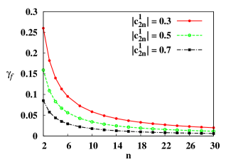
Figure 5: (Color online) Dynamics of the QD in the $1:2\cdots 2n$ bipartition for the state given in Eq. (31) in the case of the BF channel. We plot the variation of $\gamma_{f}$ as a function of $n$ for different values of $\left|c^{1}_{2n}\right|$ with $\left|c^{3}_{2n}\right|=1$, satisfying Eq. (32). All quantities are dimensionless, except the horizontal axis, which is in half of the number of particles.

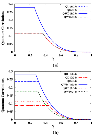
Figure 6: (Color online) (a) Freezing of QD and QWD for $\rho_{3}(x,\alpha_{1})$ with $\alpha_{1}=0.2$ and $x=0.6$. The reduced density matrix $\rho_{3}^{23}(x,\alpha_{1})$ is a BD state for which QD and QWD are identical. (b) Freezing of quantum correlations for the four-qubit state $\rho_{4}(x,\alpha_{1},\alpha_{2})$ and the reduced states $\rho_{4}^{234}$ and $\rho_{4}^{34}$ obtained from $\rho_{4}(x,\alpha_{1},\alpha_{2})$ by tracing out the first qubit and the first two qubits respectively. Here, $\alpha_{1}=0.2$, $\alpha_{2}=0.25,$ and $x=0.6$. Again, the QD and the QWD are identical for $\rho_{4}^{34}$. All quantities are dimensionless except QD, which is in bits, and QWD, which is in qubits.

IV.2 Sweeping state

We now propose another prescription for constructing general multiparty freezing states with $n$ qubits, $n$ being even or odd. Before presenting the multiparty state, let us first write down an explicit form of the bipartite state which is a CI state, and which obeys the NS condition (15) with $c_{33}^{2}+c_{01}^{2}=1$:

$$\rho_{2}(x,\alpha) = \frac{x}{2}P\left[|\psi^{2}_{0}(\alpha)\rangle+|\psi^{2}_{1}(\alpha)\rangle\right]$$ (37)

$$+\frac{1-x}{2}\left[P[|\psi^{2}_{0}(\alpha)\rangle]+P[|\psi^{2}_{1}(\alpha)\rangle]\right],$$

where $x=c_{11}$, $|\alpha|=\sqrt{\frac{1+c_{33}}{2}}$, and $P\left[|\psi\rangle\right]=|\psi\rangle\langle\psi|$. The states $|\psi^{2}_{0}(\alpha)\rangle$ and $|\psi^{2}_{1}(\alpha)\rangle$ are

$$|\psi^{2}_{0}(\alpha)\rangle = |0\rangle\otimes|\nu^{1}_{0}(\alpha)\rangle,$$ (38)

$$|\psi^{2}_{1}(\alpha)\rangle = |1\rangle\otimes|\nu^{1}_{1}(\alpha)\rangle,$$ (39)

with $|\nu^{1}_{0}(\alpha)\rangle=\alpha|0\rangle+\sqrt{1-\alpha^{2}}|1\rangle$ and $|\nu^{1}_{1}(\alpha)\rangle=\alpha|1\rangle+\sqrt{1-\alpha^{2}}|0\rangle$. The bipartite state of the form (37) can be straightforwardly extended to the tripartite case as

$$\rho_{3}(x,\alpha_{1}) = \frac{x}{2}P\left[|\psi^{3}_{0}(\alpha_{1})\rangle+|\psi^{3}_{1}(\alpha_{1})\rangle\right]$$

$$+ \frac{1-x}{2}\left[P[|\psi^{3}_{0}(\alpha_{1})\rangle]+P[|\psi^{3}_{1}(\alpha_{1})\rangle]\right],$$ (40)

with the encoding $|\psi^{3}_{0}(\alpha_{1})\rangle=|0\rangle\otimes|\nu^{2}_{0}(\alpha_{1})\rangle$ and $|\psi^{3}_{1}(\alpha_{1})\rangle=|1\rangle\otimes|\nu^{2}_{1}(\alpha_{1})\rangle$, where $|\nu^{2}_{0}(\alpha_{1})\rangle=\alpha_{1}|00\rangle+\sqrt{1-\alpha_{1}^{2}}|11\rangle$ and $|\nu^{2}_{1}(\alpha_{1})\rangle=\alpha_{1}|11\rangle+\sqrt{1-\alpha_{1}^{2}}|00\rangle$. The state in Eq. (40) can show freezing of QD as well as that of QWD in the bipartition $1:23$. Note that the marginal state $\rho_{3}^{23}(x,\alpha_{1})=\mbox{Tr}_{1}\{\rho_{3}(x,\alpha_{1})\}$ is a BD state, which satisfies the freezing condition of QD and QWD, as depicted in Fig. 6(a).

Starting from the state in Eq. (40), a four-qubit freezing state $\rho_{4}(x,\alpha_{1},\alpha_{2})$ can be generated by performing a two-qubit encoding in the qubit 3 as

$$|0\rangle\rightarrow\nu_{0}^{2}(\alpha_{2})=\alpha_{2}|00\rangle+\sqrt{1-\alpha_{2}^{2}}|11\rangle,$$

$$|1\rangle\rightarrow\nu_{1}^{2}(\alpha_{2})=\alpha_{2}|11\rangle+\sqrt{1-\alpha_{2}^{2}}|00\rangle.$$ (41)

Freezing of QD as well as QWD is observed, when measurement is made on the first qubit of $\rho_{4}(x,\alpha_{1},\alpha_{2})$. Interestingly, like the three-qubit case, all reduced density matrices of $\rho_{4}(x,\alpha_{1},\alpha_{2})$ obtained by tracing out parts from left side, starting from the qubit 1, show freezing of QD and QWD. In particular, the marginals $\rho_{4}^{234}$, $\rho_{4}^{34}$ of $\rho_{4}(x,\alpha_{1},\alpha_{2})$ show freezing of QD and QWD when the bipartition of the marginal state is considered between the first qubit and the rest of the qubits and the measurements are performed on the first qubit. The freezing of the four-qubit state and that exhibited by its three- and two-qubit reduced states are shown in Fig. 6(b).

The above procedure can be continued to generate an $n$-qubit freezing state $\rho_{n}(x,\{\alpha_{i}\})$, $i=1,\cdots,n-2,$ by applying an encoding similar to that in Eq. (41), so that the states $\{|0\rangle,|1\rangle\}$ of the qubit $(n-1)$ of $\rho_{n-1}(x,\alpha_{1},\cdots,\alpha_{n-3})$ is now replaced by $\{\nu_{0}^{2}(\alpha_{n-2}),\nu_{1}^{2}(\alpha_{n-2})\}$. The state $\rho_{n}(x,\{\alpha_{i}\})$ is a very special multipartite state for which freezing is observed for QD or QWD calculated in the bipartition $1:2...n$, with the speciality being that a freezing state of $m$ parties $(m<n)$ can be obtained from $\rho_{n}(x,\{\alpha_{i}\})$ when $n-m$ parties are traced out from the “left”  side. Each of the $n-m$ states obtained during sweeping out the qubits starting from the first qubit is also a multipartite freezing state in the bipartition $first\ qubit:rest$, when the freezing is observed by performing the measurement on the qubit $(n-m+1)$. We call the state $\rho_{n}(x,\{\alpha_{i}\})$ as the sweeping state.

V Effective freezing of quantum correlations: Freezing index

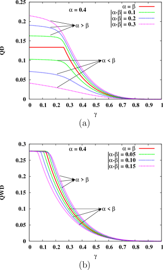
Figure 7: (Color online) The QD (a) and the QWD (b) as functions of the parametrized time $\gamma$, for the initial state given in Eq. (37) in conjunction with Eq. (42) for local BF noise. The value of the parameter $x=0.6$. All quantities are dimensionless except QD, which is in bits, and QWD, which is in qubits.

There exist classes of bipartite as well as multipartite states whose quantum coherence in the form of QD and QWD can remain constant for a finite interval of time under a noisy environment. However, such states are special in nature. Identifying these states are clearly of immense interest for efficient performance of quantum information tasks. From a practical viewpoint, it will also be interesting to find states that offer very slow decay of quantum correlations, instead of being constant, in time. The slowly decaying QD and QWD with time can be termed as “effective freezing”. To visualize such phenomena, we plot the QD and the QWD, as functions of the parametrized time $\gamma$, using the initial state given in Eq. (37) with

$$|\psi_{0}^{2}(\alpha)\rangle=|0\rangle\otimes|\nu_{0}^{1}(\alpha)\rangle,$$

$$|\psi_{1}^{2}(\beta)\rangle=|0\rangle\otimes|\nu_{1}^{1}(\beta)\rangle.$$ (42)

Note that while the QD and the QWD exactly freeze for $\alpha=\beta$, the quantities remain effectively frozen in a finite time interval, $\Delta\gamma$, for “small”  values of $|\alpha-\beta|$, as demonstrated in Fig. 7.

Freezing index: Let us now introduce a measure, which we call “freezing index”, to quantify the goodness of freezing behavior for a given trio of quantum correlation measure, $Q$, an initial state, and a decoherence channel. It necessarily depends on (i) the value, $Q^{f}$, of the frozen quantum correlation, (ii) the duration of freezing, $\Delta\gamma^{f}$, (iii) the onset of a freezing interval, and (iv) the number of freezing intervals, $N_{f}$, in the case of the existence of multiple freezing in the dynamics. The variation of the quantum correlation measure with respect to time vanishes for exact freezing while it is greater than a small number, $\delta$, named tolerance, for effective freezing. Note that a given interval is considered to be effectively frozen only if the variation of the quantum correlation measure at all points in the interval (including the end points) from the value of the measure at the starting point of the interval remains lower than the tolerance, $\delta$. In order to quantify the quality of effective freezing, we define a “freezing index”, $\eta_{f}$, for an arbitrary quantum correlation measure, as

$$\eta_{f}=\left(\sum_{i=1}^{N_{f}}\overline{Q}^{f}_{i}\left(1-\gamma_{1,i}\right)\int_{\gamma_{1,i}}^{\gamma_{2,i}}Q(\gamma)d\gamma\right)^{\frac{1}{4}},$$ (43)

where $\gamma_{1,i}$ and $\gamma_{2,i}$ are respectively the initial and final points of the “effective” freezing interval and $\overline{Q}^{f}_{i}$ is the average value of $Q$ during the freezing interval. For both QD and QWD, the maximum value of $\eta_{f}$ is unity, which occurs when maximally entangled states are sent through a noiseless channel, whereas the minimum value of $\eta_{f}$ is zero. Note also that the index can also quantify “exact” freezing phenomena, with the “effective” freezing interval being replaced by the freezing interval, and $\overline{Q}^{f}_{i}$ being replaced by $Q^{f}_{i}$, the frozen correlation value in the freezing interval $i$.

To demonstrate the freezing index, we consider the bipartite state

$$\rho_{AB} = \frac{1}{4}[I_{A}\otimes I_{B}+c_{30}\sigma_{A}^{3}\otimes I_{B}+c_{03}I_{A}\otimes\sigma_{B}^{3}$$ (44)

$$+\sum_{\alpha=1}^{3}c_{\alpha\alpha}\sigma_{A}^{\alpha}\otimes\sigma_{B}^{\alpha}],$$

where $\left|c_{30}\right|=\left|c_{03}\right|$, i.e., we have chosen the case of homogeneous magnetization in the $z$-direction. In general, QD, or QWD is found to be decaying functions of time when local BF noise is applied to the state. However, the decay of the QD can be made very slow over a certain interval of time, when the state parameters are tuned to appropriate values (see Fig. 8). For example, for low values of $c_{30}$, with properly chosen other correlators, the decay-rates of QD as well as QWD are very low, thereby ensuring a high value of $\eta_{f}$. With an increase in the magnitude of $c_{30}$, the effective freezing breaks and the correlations decay faster with time. This causes a decrease in the value of $\eta_{f}$. The dynamics of QD and QWD with increasing $c_{30}$ is represented in the inset of Fig. 8.

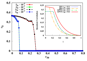
Figure 8: (Color online) Variation of the freezing index against increasing $c_{30}$ in the state in (44) for QD and QWD, for different values of $\delta$. The suffixes of $\delta$ denote whether QD or QWD is being considered as the measure. We choose $c_{11}=0.6$, $c_{22}=-0.6$, $c_{33}=1.0$, and the local BF channel for the purpose of the plot. The curves for $D$ and $W$ for a fixed value of the tolerance merge with wach other. Inset: Dynamics of QD and QWD using the state (44) as the initial state to the BF channel with different values of the magnetization $c_{30}$ The curves for $c_{30}=0.1$ for QD and QWD have merged with each other. The dimensions are as in Fig. 7.

V.1 Freezing in quantum spin models

The application of quantum information theoretic concepts and techniques to probe physical phenomena in many-body condensed matter systems has given rise to a new cross-disciplinary area of research modi_rmp_2012 ; trap_rev ; rev_xy . In this section, we investigate the dynamical behavior of the quantum correlation measures when local noise is applied to initial states that are ground states of a well-known one-dimensional (1d) quantum spin system, namely, the transverse-field anisotropic $XY$ model xy_group with periodic boundary condition. The Hamiltonian of the model is given by

$$H_{XY} = \frac{J}{2}\sum_{i=1}^{L}\left\{(1+g)\sigma_{i}^{x}\sigma_{i+1}^{x}+(1-g)\sigma_{i}^{y}\sigma_{i+1}^{y}\right\}$$ (45)

$$+h\sum_{i=1}^{L}\sigma_{i}^{z}$$

where $J$, $g$ ($-1\leq g\leq 1$), and $h$ are respectively the coupling strength, the anisotropy, and the strength of the magnetic field. The model is known to undergo a quantum phase transition at $\frac{h}{J}\equiv\lambda=\lambda_{c}\equiv 1$ xy_group ; rev_xy ; qpt_book . Two special cases of the $XY$ model are the transverse-field Ising model with $g=\pm 1$ and the isotropic $XX$ model $(g=0)$ in a transverse magnetic field. The Hamiltonian $H_{XY}$ can be diagonalized exactly in the thermodynamic limit $L\rightarrow\infty$ xy_group , for the entire range of values of the anisotropy parameter, via the successive applications of the Jordan-Wigner and the Bogoliubov transformations, and hence one can determine the nearest- and further-neighbour two-spin reduced density matrices for the ground states of the model. Since the average transverse magnetization of the ground state in the case of the $XY$ model in a transverse field does not vanish, the two-spin states obtained from the ground states do not show exact freezing of QD as well as of QWD. We address the issue of effective freezing behavior of quantum correlations in the transverse-field $XY$ model and its features in the vicinity of quantum phase transition. We determine the time evolved states obtained after local BF channels are applied to the nearest-neighbour density matrices of the ground state. In Fig. 9, we plot the QD as functions of the parametrized time $\gamma$, for a number of two-qubit initial states derived from ground states with infinite spins, for different values of $\lambda$ in the vicinity of the quantum critical point. The tolerance $\delta$ is fixed at 0.01. The QD initially decays with time for all values of $\lambda$, after which it effectively freezes for sometime before asymptotically decaying to zero. Note that the dynamics of QD at the quantum phase transition point stands out from the rest. In particular, an abrupt change in the effective freezing index at $\lambda=1$ detects the quantum phase transition. We find that the effective freezing index increases with $\lambda$ and vanishes in the paramagnetic region.

The quantum anisotropic $XY$ model with a transverse magnetic field consisting of a finite number of spins can be simulated in laboratories lab_xy and therefore, it is important to study the behavior of finite spin systems in the context of freezing dynamics. For a finite system, the transition point is again detected by an abrupt change in the value of the freezing index. The phase transition point approaches $\lambda_{c}=1$ with the increase in the size of the system as $N^{-0.729}$ i.e.,

$$\lambda_{c}^{N}=\lambda_{c}+kN^{-0.729},$$ (46)

where $k$ is a dimensionless constant (see Fig. 9).

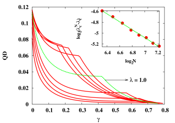
Figure 9: (Color online) QD as function of the parametrized time $\gamma$, for the two-body initial state obtained from the ground state of the infinite spin transverse Ising Hamiltonian (Eq. 45), for values of the parameter $\lambda$ on a equally spaced partition of $[0.6,1.4]$. into $8$ intervals. The curves for $\lambda=0.6$ to $0.9$ lie below the $\lambda=1.0$ curve, while those for $\lambda=1.1$ to $1.4$ lie above the $\lambda=1.0$ curve for low values of $\gamma$, say, for $\gamma<0.1$. Inset: Finite size scaling analysis for the 1d transverse Ising model using the effective freezing index as the observable. The phase transition point for an $N$ spin system approaches $\lambda=1$ as $N^{-0.729}$. All quantities are dimensionless, except QD, which is in bits, and $\log_{2}N$, which is in logarithm of the number of particles.

VI Concluding remarks

In this article, we address an interesting and as yet not entirely understood aspect of the effects on the measures of quantum correlation belonging to the information theoretic paradigm under decoherence. Specifically, we investigate the freezing of quantum correlations present in an open quantum system subjected to local noise. Our analysis identifies conditions that must be satisfied by bipartite as well as multipartite quantum states for freezing of quantum correlations in a decohering dynamics. It turns out that inhomogeneity in the magnetization of the state plays a crucial role in the freezing behavior. By comparing freezing properties of QD and QWD, we conclude that the identification of a proper measure of correlation is necessary for observation of freezing in a specific quantum state, which is clearly in contrast to earlier results. We propose a complementarity relation between the frozen value of the quantum correlation and the freezing terminal, which is the time at which the quantum correlation in the decohering state ceases to be frozen. We also demonstrate the fact that the set of states exhibiting the freezing behavior of quantum correlations is a non-convex set, containing entangled as well as separable states.

We have pointed out that apart from the quantum states that exhibit exact freezing, there also exist many quantum states which exhibit extremely slow decay of quantum correlations, and can be appropriate for information theoretic applications. We introduce a freezing index – a quantifier of the figure of merit of the dynamics with respect to freezing, which can be useful in classifying quantum correlation measures and quantum states with respect to their goodness in freezing. Applying the freezing index to the transverse-field $XY$ model, we show that the two phases of the ground state of the model have different freezing characteristics. The scaling of the freezing index with system-size is also investigated. We expect our approach to inspire novel ventures in understanding the intricacies of the dynamics of quantum correlations in open quantum systems.

- (1) R. Horodecki, P. Horodecki, M. Horodecki, and K. Horodecki, Rev. Mod. Phys. 81, 865 (2009).
- (2) K. Modi, A. Brodutch, H. Cable, T. Paterek, and V. Vedral, Rev. Mod. Phys. 84, 1655 (2012).
- (3) C. H. Bennett and S.J. Wiesner, Phys. Rev. Lett. 69, 2881 (1992); C. H. Bennett, G. Brassard, C. Crépeau, R. Jozsa, A. Peres, and W. K. Wootters, Phys. Rev. Lett. 70, 1895 (1993); R. Raussendorf and H. J. Briegel, Phys. Rev. Lett. 86, 5188 (2001); P. Walther, K. J. Resch, T. Rudolph, E. Schenck, H. Weinfurter, V. Vedral, M. Aspelmeyer, and A. Zeilinger, Nature 434, 169 (2005); H. J. Briegel, D. Browne, W. Dür, R. Raussendorf, and M. van den Nest, Nat. Phys. 5, 19 (2009).
- (4) J. M. Raimond, M. Brune, S. Haroche, Rev. Mod. Phys. 73, 565 (2001); D. Leibfried, R. Blatt, C. Monroe, and D. Wineland, Rev. Mod. Phys. 75, 281 (2003); L. M. K. Vandersypen, I.L Chuang, Rev. Mod. Phys. 76, 1037 (2005); K. Singer, U. Poschinger, M. Murphy, P. Ivanov, F. Ziesel, T. Calarco, F. Schmidt-Kaler, Rev. Mod. Phys. 82, 2609 (2010); H. Haffner, C. F. Roose, R. Blatt, Phys. Rep. 469, 155 (2008); L.-M. Duan, C. Monroe, Rev. Mod. Phys. 82, 1209 (2010); J.-W. Pan, Z.-B. Chen, C.-Y. Lu, H. Weinfurter, A. Zeilinger, M. Żukowski, Rev. Mod. Phys. 84, 777 (2012).
- (5) C. H. Bennett, D. P. DiVincenzo, C. A. Fuchs, T. Mor, E. Rains, P. W. Shor, J. A. Smolin, and W. K. Wootters, Phys. Rev. A 59, 1070 (1999); C. H. Bennett, D.P. DiVincenzo, T. Mor, P.W. Shor, J.A. Smolin, and B.M. Terhal, Phys. Rev. Lett. 82, 5385 (1999); D. P. DiVincenzo, T. Mor, P. W. Shor, J. A. Smolin, and B. M. Terhal Commun. Math. Phys. 238, 379 (2003).
- (6) A. Peres and W.K. Wootters, Phys. Rev. Lett. 66, 1119 (1991); J. Walgate, A.J. Short, L. Hardy, and V. Vedral,ibid. 85, 4972 (2000); S. Virmani, M.F. Sacchi, M.B. Plenio, and D. Markham, Phys. Lett. A 288, 62 (2001); Y.-X. Chen and D. Yang, Phys. Rev. A 64, 064303 (2001);ibid. 65, 022320 (2002); J. Walgate and L. Hardy, Phys. Rev. Lett. 89, 147901 (2002); M. Horodecki, A. Sen(De), U. Sen, and K. Horodecki, ibid. 90, 047902 (2003); W. K. Wootters, Int. J. Quantum Inf. 4, 219 (2006).
- (7) E. Knill and R. Laflamme, Phys. Rev. Lett. 81, 5672 (1998); A. Datta, A. Shaji, and C. M. Caves, Phys. Rev. Lett. 100, 050502 (2008); B. P. Lanyon, M. Barbieri, M. P. Almeida, and A. G. White, Phys. Rev. Lett. 101, 200501 (2008); cf. B. Dakić, V. Vedral, and C̃. Brukner, Phys. Rev. Lett. 105, 190502 (2010).
- (8) L. Henderson and V. Vedral, J. Phys. A 34, 6899 (2001); H. Olivier and W. H. Zurek, Phys. Rev. Lett. 88, 017901 (2001); W. H. Zurek, Rev. Mod. Phys. 75, 715 (2003).
- (9) J. Oppenheim, M. Horodecki, P. Horodecki and R. Horodecki, Phys. Rev. Lett. 89, 180402 (2002); M. Horodecki, K. Horodecki, P. Horodecki, R. Horodecki, J. Oppenheim, A. Sen(De), and U. Sen, Phys. Rev. Lett. 90, 100402 (2003); I. Devetak, Phys. Rev. A 71, 062303 (2005); M. Horodecki, P. Horodecki, R. Horodecki, J. Oppenheim, A. Sen(De), U. Sen, and B. Synak-Radtke, Phys. Rev. A 71, 062307 (2005).
- (10) Á. Rivas and S. F. Huelga, Open Quantum Systems : An Introduction (Springer Briefs in Physics, 2012); Á. Rivas, S. F. Huelga, and M. B. Plenio, Rep. Prog. Phys. 77, 094001 (2014).
- (11) K. Zyczkowski, P. Horodecki, M. Horodecki, and R. Horodecki, Phys. Rev. A 65, 012101 (2001); L. Diósi, Lec. Notes Phys. 622, 157 (2003); P. J. Dodd and J. J. Halliwell, Phys. Rev. A 69, 052105 (2004); T. Yu and J. H. Eberly, Phys. Rev. Lett. 93, 140404 (2004).
- (12) M. P. Almeida, F. de Melo, M. Hor-Meyll, A. Salles, S. P. Walborn, P. H. S. Ribeiro, and L. Davidovich, Science 316, 579 (2007); A. Salles, F. de Melo, M. P. Almeida, M. Hor-Meyll, S. P. Walborn, P. H. S. Ribeiro, and L. Davidovich, Phys. Rev. A 78, 022322 (2008); T. Yu and J. H. Eberly, Science 323, 598 (2009).
- (13) B. Bellomo, R. Lo Franco, S. Maniscalco, and G. Compagno, Phys. Rev. A 78, 060302(R) (2008); R. Lo Franco, A. D’Arrigo, G. Falci, G. Compagno, and E. Paladino, Phys. Scr. T147, 014019 (2012); A. D’Arrigo, R. Lo Franco, G. Benenti, E. Paladino, and G. Falci, Ann. Phys. 350, 211 (2014); A. D’Arrigo, G. Benenti, R. Lo Franco, G. Falci and E. Paladino, Int. J. Quant. Inf. 12, 1461005 (2014).
- (14) T. Werlang, S. Souza, F. F. Fanchini, and C. J. V. Boas, Phys. Rev. A 80, 024103 (2009); J. Maziero, L. C. Céleri, R. M. Serra, and V. Vedral, Phys. Rev. A 80, 044102 (2009); J. Maziero, T. Werlang, F. F. fanchini, L. C. Céleri, and R. M. Serra, Phys. Rev. A 81, 022116 (2010); K. Berrada, H. Eleuch, and Y. Hassouni, J. Phys. B: At. Mol. Opt. Phys. 44, 145503 (2011); A. K. Pal, and I. Bose, Eur. Phys. J. B 85:277 (2012); J. P. G. Pinto, G. Karpat, and F. F. Fanchini, Phys. Rev. A 88, 034304 (2013).
- (15) B. Wang, Z-Y Xu, Z-Q Chen, and M. Feng, Phys. Rev. A 81, 014101 (2010); F. F. Fanchini, T. Werlang, C. A. Brasil, L. G. E. Arruda, and A. O. Caldeira, Phys. Rev. A 81, 052107 (2010); F. Altintas and R. Eryigit, Phys. Lett. A 374, 4283 (2010); Z. Y. Xu, W. L. Yang, X. Xiao, and M. Feng, J. Phys. A: Math. Theor. 44, 395304 (2011); B. Bellomo, G. Compagno, R. Lo Franco, A. Ridolfo, S. Savasta, Int. J. Quant. Inf. 9, 1665 (2011); Z. Xi, X.-M. Lu, Z. Sun, and Y. Li, J. Phys. B: At. Mol. Opt. Phys. 44, 215501 (2011); R. Lo Franco, B. Bellomo, S. Maniscalco, and G. Compagno, Int. J. Mod. Phys. B 27, 1345053 (2013).
- (16) M. Daoud and R. A. Laamara, J. Phys. A: Math. Theor. 45, 325302 (2012); J. -S. Xu, K. Sun, C. -F. Li, X. -Y. Xu, G.-C. Guo, E. Andersson, R. Lo Franco, and G. Compagno, Nat. Comm. 4, 2851 (2013).
- (17) L. Mazzola, J. Piilo and S. Maniscalco, Phys. Rev. Lett. 104, 200401 (2010).
- (18) B. Aaronson, R. L. Franco, and G. Adesso, Phys. Rev. A 88, 012120 (2013).
- (19) L. Mazzola, J. Piilo, and S. Maniscalco, Int. J. Quantum Inform. 9, 981 (2011); Q -L He, J-B Xu, D-X Yao, and Y-Q Zhang, Phys. Rev. A 84, 022312 (2011); G. Karpat and Z. Gedik, Phys. Lett. A 375, 4166 (2011); Y.-Q. Lü, J.-H. An, X.-M. Chen, H.-G. Luo, and C. H. Oh, Phys. Rev. A 88, 012129 (2013); G. Karpat and Z. Gedik, Phys. Scr. T153, 014036 (2013); J.-L. Guo, H. Li, and G.-L. Long, Quant. Info. Process. 12, 3421 (2013); P. Haikka, T. H. Johnson, and S. Maniscalco, Phys. Rev. A 87, 010103(R) (2013); J. D. Montealegre, F. M. Paula, A. Saguia, and M. S. Sarandy, Phys. Rev. A 87, 042115 (2013).
- (20) J.-S. Xu, X.-Y. Xu, C.-F. Li, C.-J. Zhang, X.-B. Zou and G.-C. Guo, Nature Commun. 1, 7 (2010); R. Auccaise, L. C. Céleri, D. O. Soares-Pinto, E. R. deAzevedo, J. Maziero, A. M. Souza, T. J. Bonagamba, R. S. Sarthour, I. S. Oliveira and R. M. Serra, Phys. Rev. Lett. 107, 140403 (2011); F. M. Paula, I. A. Silva, J. D. Montealegre, A. M. Souza, E. R. deAzevedo, R. S. Sarthour, A. Saguia, I. S. Oliveira, D. O. Soares-Pinto, G. Adesso, and M. S. Sarandy, Phys. Rev. Lett. 111, 250401 (2013); X. Rong, F. Jin, Z. Wang, J. Geng, C. Ju, Y. Wang, R. Zhang, C. Duan, M. Shi, and J. Du, Phys. Rev. B 88, 054419 (2013).
- (21) D. A. Lidar, Adv. Chem. Phys. 154, 295 (2014).
- (22) D. Kielpinski, V. Meyer, M. A. Rowe, C. A. Sackett, W. M. Itano, C. Monroe, D. J. Wineland, Science 291, 1013 (2001).
- (23) E. Lieb, T. Schultz, and D. Mattis, Ann. Phys. 16, 407 (1961); E. Barouch, B.M. McCoy, and M. Dresden, Phys. Rev. 2, 1075 (1970); E. Barouch and B.M. McCoy, Phys. Rev. 3, 786 (1971).
- (24) M. Schechter and P. C. E. Stamp, Phys. Rev. B 78, 054438 (2008).
- (25) X. -L. Deng, D. Porras, and J. I. Cirac, Phys. Rev. A 72, 063407 (2005).
- (26) M. Lewenstein, A. Sanpera, V. Ahufinger, B. Damski, A.Sen(De), and U. Sen, Adv. Phys. 56, 243 (2007).
- (27) R. Islam, E. E. Edwards, K. Kim, S. Korenblit, C. Noh, H. Carmichael, G.-D. Lin, L.-M. Duan, C.-C. Joseph Wang, J. K. Freericks, and C. Monroe, Nature Commun. 2, 377 (2011); J. Struck, M. Weinberg, C. Ölschläger, P. Windpassinger, J. Simonet, K. Sengstock, R. Höppner, P. Hauke, A. Eckardt, M. Lewenstein, and L. Mathey, Nature Physics 9, 738 (2013), and references therein.
- (28) N. J. Cerf, C. Adami, Phys. Rev. Lett. 79, 5194 (1997); B. Groisman, S. Popescu, and A. Winter, Phys. Rev. A 72, 032317 (2005).
- (29) S. Luo, Phys. Rev. A 77, 042303 (2008).
- (30) T. Yu and J. H. Eberly, Phys. Rev. Lett. 97, 140403 (2006).
- (31) U. Fano, Rev. Mod. Phys. 55, 855 (1983).
- (32) Y. Huang, Phys. Rev. A 88, 014302 (2013); M. Namkung, J. Chang, J. Shin, and Y. Kwon, arXiv: 1404.6329 [quant-ph] (2014).
- (33) B. Li, Z.-X. Wang, and S.-M. Fei, Phys. Rev. A 83, 022321 (2011).
- (34) L. Amico, R. Fazio, A. Osterloh, and V. Vedral, Rev. Mod. Phys. 80, 517 (2008); J. I. Latorre, and A. Rierra, J. Phys. A 42, 504002 (2009); J. Eisert, M. Cramer, and M. B. Plenio, Rev. Mod. Phys. 82, 277, (2010).
- (35) B. K. Chakrabarti, A. Dutta, and P. Sen, Quantum Ising Phases and Transitions in Transverse Ising Models (Springer, Heidelberg, 1996); S. Sachdev, Quantum Phase Transitions (Cambridge University Press, Cambridge, 2011); S. Suzuki, J. -I. Inou, B. K. Chakrabarti, Quantum Ising Phases and Transitions in Transverse Ising Models (Springer, Heidelberg, 2013).