Molecular modelling and simulation of the surface tension of real quadrupolar fluids

Abstract

Molecular modelling and simulation of the surface tension of fluids with force fields is discussed. 29 real fluids are studied, including nitrogen, oxygen, carbon dioxide, carbon monoxide, fluorine, chlorine, bromine, iodine, ethane, ethylene, acetylene, propyne, propylene, propadiene, carbon disulfide, sulfur hexafluoride, and many refrigerants. The fluids are represented by two-centre Lennard-Jones plus point quadrupole models from the literature. These models were adjusted only to experimental data of the vapour pressure and saturated liquid density so that the results for the surface tension are predictions. The deviations between the predictions and experimental data for the surface tension are of the order of 20 %. The surface tension is usually overestimated by the models. For further improvements, data on the surface tension can be included in the model development. A suitable strategy for this is multi-criteria optimization based on Pareto sets. This is demonstrated using the model for carbon dioxide as an example.

1 Introduction

In classical phenomenological thermodynamics following Gibbs [1], interfacial properties are considered as excess contributions which are assigned to a formal dividing surface. In this way, the surface tension is obtained from the excess free energy with respect to a hypothetical system that does not contain an interface, consisting of the bulk phases in thermodynamic equilibrium only. Theorems that hold for the bulk properties can be immediately applied to interfacial thermodynamics, yielding fundamental relations such as the Gibbs adsorption equation [1, 2].

In interfacial thermodynamics, the Gibbs dividing surface represents the highest level of abstraction. Being strictly two-dimensional, the dividing surface does not have any volume, and its internal structure is not considered. While this simplifies the theoretical framework, it neglects physical phenomena which are important for understanding fluid interfaces. Since van der Waals [3], it has been understood that such a purely empirical description can benefit from a theory of the fluid interface as a continuous region connecting two phases.

Thermodynamically, the internal structure of the interface, such as its thickness, can be considered by generalized versions of the Gibbs approach, e.g. as devised by Guggenheim [4] or from more recent work [5, 6]. Furthermore, investigations based on statistical mechanics can provide a more detailed insight by describing the thermodynamics of interfaces in terms of their molecular structure [7, 8]. In particular, density functional theory (DFT) in combination with molecular equations of state was found to be a viable approach for interfacial properties of pure fluids [9, 10] as well as mixtures [11, 9]. In combination with simple expressions for the free energy, DFT yields analytical results such as the well-known approximation of the density profile by a hyperbolic tangent [12].

Molecular dynamics (MD) simulation, on the other hand, is based on the equations of motion from classical mechanics. While it is computationally more expensive, systems containing up to trillions of molecules can today be simulated on supercomputers, employing numerically convenient pair potentials [13, 14]. With relatively few model parameters, which can be adjusted to experimental data, molecular pair potentials are highly reliable for extrapolating and predicting a wide variety of fluid properties consistently [15, 16]. Both static and dynamic properties can be computed by MD simulation [17, 18, 19], for bulk phases as well as for heterogeneous systems [20, 21]. Even heat and mass transfer at fluid interfaces is well accessible to molecular dynamics [22, 23].

In a homogeneous bulk fluid, the long-range part of the force field acting on a single molecule averages out beyond a certain cutoff radius $r_{\mathrm{c}}$, and straightforward mean-field approximations can be applied to compute the long-range contribution to the energy and the pressure [24]. For simulations in the canonical ensemble, these corrections can be treated statically for the Lennard-Jones potential, and even for dipolar molecules [25], i.e. they have to be computed only once and do not change over time. However, molecular simulation of heterogeneous systems is more challenging, since the approximations behind the most straightforward techniques for homogeneous systems, e.g. the reaction field method [26], break down in an anisotropic environment.

At a vapour-liquid interface, a volume integral over a short-range interaction such as dispersion, which decays with $r_{ij}^{-6}$ in terms of the intermolecular distance $r_{ij}$, can yield a significant contribution, of the order of $r_{\mathrm{c}}^{-3}$, to the potential energy as well as the surface tension [27]. Various algorithms have been devised to compute such effects efficiently and in a scalable way [28, 29], facilitating the massively-parallel MD simulation of heterogeneous systems with large numbers of particles [30, 31].

On the molecular level, the surface tension $\gamma$ can be considered in different ways, based on mechanical and thermodynamic approaches. Thermodynamically, the surface tension is defined by the free energy change related to a differential variation of the surface area. Such differential excess free energies can be determined by test-area simulation [32, 33], whereas approaches based on grand-canonical sampling yield the absolute excess free energy associated with the interface [34, 35, 36, 37, 38].

Mechanically, an interfacial tension causes a local stress, i.e. a negative pressure, which acts in the direction tangential to the interface. For the vapour-liquid surface tension at curved interfaces, mechanical and thermodynamic methods lead to contradicting results [39, 40, 38], and thermodynamic statements cannot be based on the mechanically defined value of $\gamma$ directly. In case of planar fluid interfaces, however, the mechanical and thermodynamic approaches are rigorously equivalent, and the mechanical approach, which is employed here, can be straightforwardly implemented in terms of the intermolecular virial [41]. If periodic boundary conditions are employed and the canonical ensemble is simulated, the surface tension is immediately related to the deviation between the normal and tangential components of the pressure tensor.

Accurate molecular simulation results for the surface tension require an adequate consideration of the long-range contribution, which is sometimes nonetheless absent from works reporting such values [16, 42]. Molecular models for which the surface tension has recently been evaluated reliably include carbon dioxide [43, 44], which is also considered in the present work, water models [45, 43], and several other molecular fluids [46, 47]. Comparing model predictions to experimental data, deviations were found to be of the order of 10 to 20 % for various molecular models from the literature [43, 46, 47] and typically of the order of 50 % for water models [45].

However, no systematic evaluation of $\gamma$ by MD simulation of an entire class of molecular models has been conducted so far. This is the aim of the present work, focusing on a simple, but powerful class of models for real fluids from the literature. Vrabec et al. [48] and Stoll et al. [49] developed molecular models of the two-centre Lennard-Jones plus point quadrupole (2CLJQ) type for 29 real compounds, including air components, halogens, hydrocarbons, and refrigerants. In previous work, these models were also applied successfully to binary [50] and ternary mixtures [51]. The vapour-liquid equilibrium (VLE) behaviour of the 2CLJQ model fluid has been studied systematically [52], serving as the basis for a molecular equation of state which contains an explicit contribution of the quadrupole moment [53].

A correlation for the surface tension of the 2CLJQ model fluid from previous work [54] is extended by new MD simulations in the present work. On this foundation, the predictive capacity regarding the surface tension of the planar vapour-liquid interface is assessed here for these models, which were adjusted to VLE properties of the bulk fluids only [48, 49], i.e. interfacial properties were not taken into account for the parametrization.

For the present MD simulations of the surface tension, an efficient algorithm is employed to compute the contribution of the long-range correction [29], combining an integration over planar slabs [27] with a centre-of-mass cutoff for multi-site models [55]. The obtained vapour-liquid surface tension is entirely predictive, and a comparison with experimental data can serve to validate or improve the molecular models. The surface tension predicted by these models has not been studied previously, except for molecular nitrogen and oxygen, where Eckelsbach et al. [47] found a deviation of about 15 % between model properties and experimental data. The present work confirms this result and considers the whole set of 2CLJQ models of real fluids systematically.

The agreement of a molecular model with real fluid properties, e.g. for the surface tension, can be improved by taking the respective experimental data explicitly into account when the model parameters are optimized. In the literature, various optimization approaches employing a single objective function can be found [16, 64, 65, 66]. Thereby, the objective function is designed to represent the quality of several thermodynamic properties simultaneously, and specific preferences of the model developer are expressed by setting weights for these properties. To find the minimum of the objective function, gradient based algorithms can be applied, e.g. starting from a reference model from literature or based on quantum chemical calculations. The derivative of the objective function over the model parameters is evaluated and the steepest descent defines the change in the parameters.

In the present work, a multi-criteria optimization approach is used instead to identify the Pareto set, i.e. the set of molecular models which cannot be altered without ranking worse according to at least one of the considered criteria. Here, several objective functions can be defined and optimized simultaneously. Since different criteria generally represent conflicting goals, it is not possible to find a molecular model leading to a minimum in all objective functions. Instead, the set of Pareto optimal molecular models (i.e. the Pareto set), is determined by which all possible compromises between the objective functions are accessible. Knowing the Pareto set, one can choose the model best suited for a particular application. In previous work of Stöbener et al. [59], this approach was applied to the single-centre Lennard-Jones fluid, which has two model parameters. In the present work, the four-dimensional parameter space of the 2CLJQ model is explored, yielding a comprehensive description of CO₂ in terms of three objective functions, corresponding to three thermodynamic properties: The vapour pressure, the saturated liquid density, and the surface tension.

This article is structured as follows: In Section 2, the simulation method is briefly described. Simulation results on the predictive power of the 2CLJQ molecular models from the literature, regarding the surface tension, are presented in Section 3. Multi-criteria optimization of molecular models is discussed and applied to carbon dioxide in Section 4, leading to the conclusion in Section 5.

2 Simulation Method

The molecular models in the present work consist of two identical Lennard-Jones sites and a point quadrupole in the centre of mass. The Lennard-Jones potential is described by

$$u_{ij}^{\rm LJ}=4\epsilon\left[\left(\frac{\sigma}{r_{ij}}\right)^{12}-\left(\frac{\sigma}{r_{ij}}\right)^{6}\right],$$ (1)

with the size parameter $\sigma$ and the energy parameter $\epsilon$. The quadrupole-quadrupole interaction is described by

$$u_{ij}^{\rm Q}=\frac{1}{4\pi\epsilon_{0}}\frac{3}{4}\frac{Q^{2}}{r_{ij}^{5}}f\left(\omega\right),$$ (2)

where $\epsilon_{0}$ is the electric constant, $Q$ is the quadrupole moment of the molecules, and $f\left(\omega\right)$ is a dimensionless angle-dependent expression [56].

The surface tension $\gamma$ is obtained from the difference between the normal and tangential contributions to the virial $\Pi_{N}$ $-$ $\Pi_{T}$, which is equivalent to the integral over the differential pressure $p_{N}$ $-$ $p_{T}$

$$\gamma=\frac{1}{2A}\left(\Pi_{N}-\Pi_{T}\right)=\frac{1}{2}\int_{-\infty}^{\infty}{\rm d}y\left(p_{N}-p_{T}\right),$$ (3)

where 2A denotes the area of the two dividing surfaces in the simulation volume with periodic boundary conditions [57, 27] and $y$ is the direction normal to the interface.

Further technical details of the simulation method are described in the Appendix.

3 Prediction of the surface tension of 29 real fluids by molecular simulation

In the following the results for the surface tension as predicted by the models of Vrabec et al. [48] and Stoll et al. [49] are presented and compared to DIPPR correlations which were adjusted to experimental data (the employed model parameters are given in the Appendix). The average deviation between the DIPPR correlation and the experimental data is below 1 $\%$ for most of the fluids studied in the present work, except CO₂ with an average deviation of about 4 $\%$ and R115 with about 1.8 $\%$ [58].

Figure 1 shows the surface tension of air components as a function of the temperature. The surface tension of N₂, O₂ and CO is overestimated by about 15 %, while for CO₂ that number is 26 $\%$. The results for the surface tension of N₂ and O₂ are similar to results of Eckelsbach et al. [47].

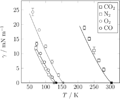
Figure 1: Surface tension of air components as a function of the temperature. The open symbols are simulation results from the present work. The solid lines represent DIPPR correlations [58], based on experimental data, and the filled symbols denote the respective critical point.

Figure 2 shows the surface tension of some refrigerants as a function of the temperature. The surface tension is again overestimated, but the molecular models predict the different slopes of the surface tension curve well, even though the critical temperatures of R114 and R134 are only 26 K apart.

Figure 2: Surface tension of various refrigerants as a function of the temperature. The open symbols are simulation results from the present work. The solid lines represent DIPPR correlations [58], based on experimental data, and the filled symbols denote the respective critical point.

Figure 3 shows the surface tension of halogens as a function of the temperature. The prediction by the molecular models are about as good as in the cases discussed above except for I₂. Experimental data for the surface tension of I₂ are only available between about 390 and 425 K, while the critical point is slightly above 800 K. The extrapolation of the DIPPR correlation may be unreliable. In the temperature range where experimental data are available, the deviation between the prediction by molecular simulation and the experimental data is about 19 %, and hence in the range as observed for the other studied systems.

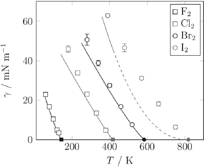
Figure 3: Surface tension of halogens as a function of the temperature. The open symbols are simulation results from the present work. The solid lines represent DIPPR correlations [58], based on experimental data, and the filled symbols denote the respective critical point. The dashed line for I₂ indicates that experimental data are only available up to 425 K.

Figure 4 shows the surface tension of halogenated carbons. The molecular model for C₂F₄ is the only model that underestimates the surface tension.

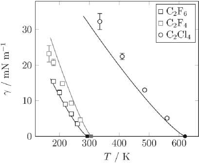
Figure 4: Surface tension of halogenated carbons as a function of the temperature. The open symbols are simulation results from the present work. The solid lines represent DIPPR correlations [58], based on experimental data, and the filled symbols denote the respective critical point.

The surface tension of all other compounds investigated in the present work are shown in the Appendix.

All in all the surface tension of 29 real fluids was studied in the present work. The deviation between the prediction by the molecular models of Vrabec et al. [48] and Stoll et al. [49] which were not adjusted to experimental data for the surface tension is of the order of 20 %. The surface tension is overestimated by the models in most cases. Nevertheless, considering that only data for the saturated liquid density and the vapour pressure were used for the model development, this is a good agreement.

To increase the quality of the molecular models in terms of the surface tension, they have to be reoptimized, taking the surface tension into account.A suitable way for doing this is multi-criteria optimization.

4 Model Optimization

In the following a multi-criteria optimization of the molecular model of Vrabec et al. [48] for CO₂ is discussed. Besides the saturated liquid density and the vapour pressure, which were already taken into account by Vrabec et al. [48], now also the surface tension is considered.

Three objective functions $g_{i}$, depending on the molecular model parameters, are considered. Each objective function represents the relative mean deviation for one relevant property $O$, i.e. the saturated liquid density, the vapour pressure and the surface tension,

$$g_{i}=\delta O=\sqrt{\frac{1}{N}\sum_{j=1}^{N}\left(\frac{O^{\rm exp}(T_{j})-O^{\rm sim}(T_{j},\sigma,\epsilon,L,Q}{O^{\rm exp}(T_{j})}\right)^{2}},$$ (4)

where $O^{\rm exp}$ are properties calculated by DIPPR correlations and $O^{\rm sim}$ are properties calculated by correlations to simulation data.

The DIPPR correlations are based on the entire set of experimental data available for each fluid and deviate from the individual data points to a certain extent. The relative mean deviations between the simulation data and the correlations are about 0.4 % for the saturated liquid density, about 1.8 $\%$ for the vapour pressure [52] and about 1.9 % for the surface tension [54]. The temperature values are equidistantly spaced from the triple point temperature up to 95 $\%$ of the critical temperature in 5 K steps.

Figure 5 shows the influence of increasing one molecular model parameter by 5 %, while the other parameters are kept constant, on the surface tension. The base line corresponds to the model parameters from Vrabec et al. [48]. Increasing one energy parameter, $\epsilon$ or $Q$, increases the surface tension value, while increasing the size parameter, $\sigma$ or $L$, decreases the surface tension value. The corresponding phase diagram and vapour pressure curve are shown in the Appendix.

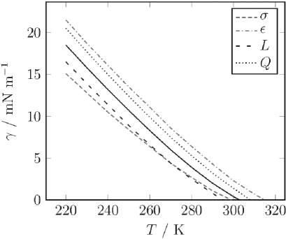
Figure 5: Surface tension of CO₂. The solid line is the base line, representing the molecular model of Vrabec et al. [48]. The dotted and dashed lines show the effect of an increase of 5 % in the corresponding model parameter.

The Pareto set is obtained by brute force sampling of the parameter space. Therefore lower and upper bounds were defined for the parameters, $\sigma$, $\epsilon$, $L$, $Q$, such that the whole Pareto set is found. The sampled grid is 60 $\times$ 60 $\times$ 60 $\times$ 60 points. Based on the correlations of Stoll et al. [52] and Werth et al. [54] the relative mean deviations between the simulation data and the experimental data are determined. The comparison of all molecular models generates the Pareto set.

Figure 6 shows the Pareto set in the parameter space on the left hand side and the objective space on the right hand side, represented by the deviation in the saturated liquid density, the vapour pressure and the surface tension. From Figure 6 it can be seen which parameter values correspond to an optimum in two objective functions. The molecular model of Vrabec et al. [48] for CO₂ (upward triangle in Figure 6) is found to lie on the Pareto set. It represents a compromise which is excellent in the vapour pressure and the saturated liquid density, but poor in the surface tension (cf. Table 1). Some other compromises taken from the Pareto set are discussed in the following (parameters cf. Table 2). It is possible to find models which are good in the vapour pressure and the surface tension, but poor in the saturated liquid density (e.g. model $\gamma-p$ designated by a circle in Figure 6) or models which are good in the saturated liquid density and the surface tension, but poor in the vapour pressure (e.g. model $\gamma-\rho$ designated by diamond in Figure 6). Contrarily to the model of Vrabec et al. [48] these choices are not attractive as they yield very high deviations for the quantity which is described poorly, cf. Table 1. Taking the model of Vrabec et al. [48] as a starting point, the knowledge of the Pareto set enables finding compromises which are distinctly better in the surface tension at some expense in the quality for the saturated liquid density and the vapour pressure, (e.g. model $\gamma-\rho-p$ by downward triangle in Figure 6). Note that all models discussed in the present section are optimal according to the definition given by Pareto.

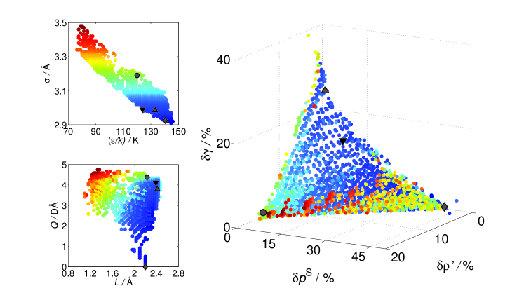
Figure 6: Pareto set of the 2CLJQ molecular models for CO₂ in the parameter space, represented by the Lennard-Jones parameters $\sigma$ and $\epsilon$ (left top) and the model parameters $Q$ and $L$ (left bottom), and the objective space (right): deviations in the surface tension, the saturated density and the vapour pressure. The upward triangle denotes the molecular model of Vrabec et al. [48], the circle ($\gamma-p$) and the diamond ($\gamma-\rho$) denote the optimizations in two objective functions and the downward triangle denotes the new optimized molecular model ($\gamma-\rho-p$). The colors represent the numerical value of $\sigma$ and connect the points in the parameter and the objective space.

	$\delta\rho^{\prime}$ / %	$\delta p$ / %	$\delta\gamma$ / %
Vrabec et al. [48]	0.36	3.68	26.4
$\gamma-p$	14.4	2.60	5.42
$\gamma-\rho$	0.77	41.6	4.21
$\gamma-\rho-p$	0.86	9.24	12.3

Table 1: Relative mean deviation in the saturated liquid density, the vapour pressure and the surface tension of the molecular models for CO₂ from Vrabec et al. [48] and the optimized versions from the present work.

	$\sigma$ / Å	$\epsilon$ / $k_{\rm B}$	$L$ / Å	$Q$ / DÅ
Vrabec et al. [48]	2.9847	133.22	2.4176	3.7938
$\gamma-p$	3.19	120	2.233	4.3766
$\gamma-\rho$	2.925	140.5	2.144	-
$\gamma-\rho-p$	2.99	124	2.392	4.1091

Table 2: Parameters of the molecular models for CO₂ from Vrabec et al. [48] and the optimized versions from the present work.

Table 2 shows the molecular model parameters for CO₂ which were selected from the Pareto set of the 2CLJQ model class as described above. The molecular model $\gamma-\rho$ does not have a quadrupole moment and the quadrupole moments of the other models are slightly larger than the value used of Vrabec et al. [48]. Experimental data for the quadrupole moment are between 1.64 and 4.87 DÅ [56]. The experimental C=O distance is 1.15 Å [68]. The deviation between this value and $L/2$ of the molecular models is less than 5 %.

More detailed information on the representation of the different thermodynamic properties by the models discussed above is available in the Appendix.

5 Conclusion

In the present work, the ability of molecular models to predict the surface tension of real compounds was tested. 29 models of the 2CLJQ type which were parameterized using only experimental data of the saturated liquid density and the vapour pressure were used to predict the surface tension. The deviation between the prediction and the experimental data is usually of the order of 20 % and the surface tension is overestimated. These deviations are not large considering that they refer to data along almost the entire vapour pressure curve of the studied compounds. And that both the simulation results and the experimental data are subject of errors which are of the order of 1 % and 5 % respectively.

Increasing the quality of the molecular models requires including the surface tension in the model optimization procedure. Here a multi-criteria optimization using a Pareto approach was used to optimize a molecular model for CO₂ tailored for particular applications. The Pareto approach can be generally applied to include the surface tension in the model development. A suitable multi-criteria optimization approach, based on constructing the Pareto set for the considered model class with respect to multiple thermodynamic properties, was presented here and applied to carbon dioxide. With a compromise model selected from the Pareto set, fair agreement is obtained for vapour-liquid equilibrium properties of the bulk fluid as well as the surface tension.

Acknowledgment. The authors acknowledge financial support from BMBF within the SkaSim project and from DFG within the Collaborative Research Centre MICOS (SFB 926) as well as the Reinhart Kosseleck Programme (grant HA 1993/15-1). They thank Doros Theodorou for his encouragement as well as Wolfgang Eckhardt, Manfred Heilig, Maximilian Kohns, Kai Langenbach, Gábor Rutkai, and Jadran Vrabec for fruitful discussions. The present work was conducted under the auspices of the Boltzmann-Zuse Society of Computational Molecular Engineering (BZS), and the MD simulations were carried out on the SuperMUC at Leibniz-Rechenzentrum Garching within the large-scale scientific computing project pr83ri.

Appendix

Simulation Details

The simulations were performed with the molecular dynamics code $ls1$ $MarDyn$ [61] in the canonical ensemble with $N$ = 16 000 particles. The parameters of the molecular models of Vrabec et al. [48] and Stoll et al. [49] are given in Table 3. The equation of motion was solved by a leapfrog integrator [62] with a time step of $\Delta t$ = 1 fs. The elongation of the simulation volume normal to the interface was 80 $\sigma$ and the thickness of the liquid film in the centre of the simulation volume was 40 $\sigma$ to account for finite size effects [63]. The elongation in the other spatial directions was at least 20 $\sigma$.

Name	Formula	CAS RN	$\sigma$ / Å	$\epsilon$ / $k_{\rm B}$	$L$ / Å	$Q$ / DÅ	Author
Florine	F2	7782-41-4	2.8258	52.147	1.4129	0.8920	[48]
Chlorine	Cl2	7782-50-5	3.4016	160.86	1.9819	4.2356	[48]
Bromine	Br2	7726-95-6	3.5546	236.76	2.1777	4.8954	[48]
Iodine	I2	7553-56-2	3.7200	371.47	2.6784	5.6556	[48]
Nitrogen	N2	7727-37-9	3.3211	34.897	1.0464	1.4397	[48]
Oxygen	O2	7782-44-7	3.1062	43.183	0.9699	0.8081	[48]
Carbon dioxide	CO2	124-38-9	2.9847	133.22	2.4176	3.7938	[48]
Carbon disulfide	CS2	75-15-0	3.6140	257.68	2.6809	3.8997	[48]
Ethane	C2H6	74-84-0	3.4896	136.99	2.3762	0.8277	[48]
Ethylene	C2H4	74-85-1	3.7607	76.950	1.2695	4.3310	[48]
Acetylene	C2H2	74-86-2	3.5742	79.890	1.2998	5.0730	[48]
R116	C2F6	76-16-4	4.1282	110.19	2.7246	8.4943	[48]
R1114	C2F4	116-14-3	3.8611	106.32	2.2394	7.0332	[48]
R1110	C2Cl4	127-18-4	4.6758	211.11	2.6520	16.143	[48]
Propadiene	C3H4	463-49-0	3.6367	170.52	2.4958	5.1637	[48]
Propyne	C3H4	74-99-7	3.5460	186.43	2.8368	5.7548	[48]
Propylene	C3H6	115-07-1	3.8169	150.78	2.5014	5.9387	[48]
R846	SF6	2551-62-4	3.9615	118.98	2.6375	8.0066	[48]
R14	CF4	75-73-0	3.8812	59.235	1.3901	5.1763	[48]
R10	CCl4	56-23-5	4.8471	142.14	1.6946	14.346	[48]
Carbon monoxide	CO	630-08-0	3.3344	36.713	1.1110	1.9170	[49]
R113	CFCl2-CF2Cl	76-13-1	4.5207	217.08	3.6166	12.984	[49]
R114	CBrF2-CBrF2	76-14-2	4.3772	183.26	3.5018	11.456	[49]
R115	CF3-CF2Cl	76-15-3	4.1891	155.77	3.3513	9.2246	[49]
R134	CHF2-CHF2	359-35-3	3.7848	170.46	3.0278	7.8745	[49]
R30B2	CH2Br2	74-95-3	3.8683	274.97	3.0946	9.2682	[49]
R150B2	CH2Br-CH2Br	106-93-4	4.1699	302.33	3.3359	10.903	[49]
R114B2	CBrF2-CBrF2	124-73-2	4.5193	218.40	3.6154	12.822	[49]
R1120	CHCl=CCl2	79-01-6	4.4120	201.03	2.6357	13.624	[49]

Table 3: Parameters of the molecular models of Vrabec et al. [48] and Stoll et al. [49].

The equilibration was conducted for 500 000 time steps and the production runs for 2 500 000 time steps to reduce statistical uncertainties. The statistical errors were estimated to be three times the standard deviation of five block averages, each over 500 000 time steps. The saturated densities and the vapour pressure were calculated as an average over the respective phases excluding the area close to the interface.

The cutoff radius was set to 5 $\sigma$ and a centre-of-mass cutoff scheme was employed. The Lennard-Jones interactions were corrected with a slab-based long range correction (LRC) [29]. The quadrupole was assumed to have no preferred orientation, which yields a vanishing LRC contribution. Following Eq. (3), the surface tension was computed immediately from the deviation between the normal and tangential diagonal components of the overall pressure tensor for the whole system. Thereby, the tangential pressure $p_{T}$ was determined by averaging over the two tangential components of the pressure tensor.

Additional simulation results

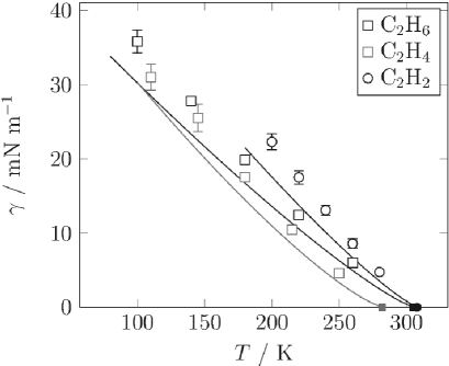
Figure 7: Surface tension of hydrocarbons as a function of the temperature. The open symbols are simulation results from the present work. The solid lines represent DIPPR correlations [58], based on experimental data, and the filled symbols denote the respective critical point.

Figure 8: Surface tension of hydrocarbons as a function of the temperature. The open symbols are simulation results from the present work. The solid lines represent DIPPR correlations [58], based on experimental data, and the filled symbols denote the respective critical point.

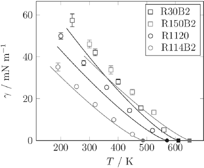
Figure 9: Surface tension of refrigerants as a function of the temperature. The open symbols are simulation results from the present work. The solid lines represent DIPPR correlations [58], based on experimental data, and the filled symbols denote the respective critical point.

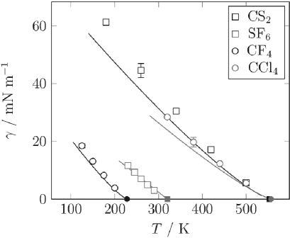
Figure 10: Surface tension of various fluids as a function of the temperature. The open symbols are simulation results from the present work. The solid lines represent DIPPR correlations [58], based on experimental data, and the filled symbols denote the respective critical point.

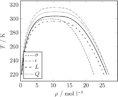
Figure 11: Saturated densities of CO₂. The solid line is the base line, representing the molecular model of Vrabec et al. [48]. The dotted and dashed lines show the effect of an increase of 5 % in the corresponding model parameter.

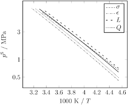
Figure 12: Vapour pressure of CO₂. The solid line is the base line, representing the molecular model of Vrabec et al. [48]. The dotted and dashed lines show the effect of an increase of 5 % in the corresponding model parameter.

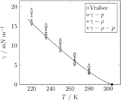
Figure 13: Surface tension of CO₂ as a function of the temperature. Comparison between molecular models optimized to the surface tension and the vapour-pressure ($\gamma-p$), the surface tension and the saturated liquid density ($\gamma-\rho$), the optimized model ($\gamma-\rho-p$) and a previous model of Vrabec et al. [48], cf. Table 2. The solid line represents the DIPPR correlation [58], based on experimental data, and the filled symbol denotes the critical point.

Figure 14: Saturated densities of CO₂. Comparison between molecular models optimized to the surface tension and the vapour-pressure ($\gamma-p$), the surface tension and the saturated liquid density ($\gamma-\rho$), the optimized model ($\gamma-\rho-p$) and a previous model of Vrabec et al. [48], cf. Table 2. The solid line represents the DIPPR correlation [58], based on experimental data, the dashed line is based on an equation of state [67]. Error bars are within symbol size.

Figure 15: Vapour pressure of CO₂ as a function of the temperature. Comparison between molecular models optimized to the surface tension and the vapour-pressure ($\gamma-p$), the surface tension and the saturated liquid density ($\gamma-\rho$), the optimized model ($\gamma-\rho-p$) and a previous model of Vrabec et al. [48], cf. Table 2. The solid line represents the DIPPR correlation [58], based on experimental data.

References

- [1] J. W. Gibbs, Transact. Connecticut Acad. Arts Sciences 3 (1876) 108–248, (1878) 343–524.
- [2] R. A. Alberty, Langmuir 11 (9) (1995) 3598–3600.
- [3] J. D. van der Waals, Ph.D. thesis, Universiteit Leiden (1873).
- [4] E. A. Guggenheim, Transact. Faraday Soc. 35 (1940) 397–412.
- [5] T. Frolov, Y. Mishin, J. Chem. Phys. 131 (2009) 054702.
- [6] B. B. Laird, R. Davidchack, J. Chem. Phys. 132 (2010) 204101.
- [7] D. Henderson, F. F. Abraham, J. A. Barker, Mol. Phys. 31 (4) (1976) 1291–1295.
- [8] M. Xu, C. Zhang, Z. Du, J. Mi, J. Phys. Chem. B 112 (22) (2012) 6514–6521.
- [9] S. Jain, A. Dominik, W. G. Chapman, J. Chem. Phys. 127 (2007) 244904.
- [10] J. Gross, J. Chem. Phys. 131 (2009) 204705.
- [11] H. Kahl, S. Enders, Phys. Chem. Chem. Phys. 4 (6) (2002) 931–936.
- [12] B. U. Felderhof, Physica 48 (4) (1970) 541–560.
- [13] T. C. Germann, K. Kadau, Int. J. Mod. Phys. C 19 (9) (2008) 1315–1319.
- [14] W. Eckhardt, A. Heinecke, R. Bader, M. Brehm, N. Hammer, H. Huber, H.-G. Kleinhenz, J. Vrabec, H. Hasse, M. Horsch, M. Bernreuther, C. W. Glass, C. Niethammer, A. Bode, J. Bungartz, in: Supercomputing (Proc. 28th ISC), no. 7905 in LNCS, Springer, Heidelberg, 2013, pp. 1–12.
- [15] P. Ungerer, C. Nieto Draghi, B. Rousseau, G. Ahunbay, V. Lachet, J. Mol. Liq. 134 (2007) 71–89.
- [16] B. Eckl, J. Vrabec, H. Hasse, Fluid Phase Equilib. 274 (1–2) (2008) 16–26.
- [17] S. K. Bhatia, D. Nicholson, Phys. Rev. Lett. 90 (2003) 016105.
- [18] R. J. Allen, C. Valeriani, P. R. ten Wolde, J. Phys.: Cond. Mat. 21 (46) (2009) 463102.
- [19] G. Guevara Carrión, H. Hasse, J. Vrabec, in: Multiscale Molecular Methods in Applied Chemistry, no. 307 in Topics in Current Chemistry, Springer, Heidelberg, 2012, pp. 201–249.
- [20] J. Vrabec, G. K. Kedia, G. Fuchs, H. Hasse, Mol. Phys. 104 (9) (2006) 1509–1527.
- [21] E. A. Müller, Cur. Opin. Chem. Eng. 2 (2013) 223–228.
- [22] G. Strotos, M. Gavaises, A. Theodorakakos, G. Bergeles, Int. J. Heat Mass Transfer 51 (2008) 1516–1529.
- [23] A. Lotfi, J. Vrabec, J. Fischer, Int. J. Heat Mass Transf. 73 (2014) 303–317.
- [24] M. P. Allen, D. J. Tildesley, Computer Simulation of Liquids, Clarendon, Oxford, 1987.
- [25] B. Saager, J. Fischer, M. Neumann, Mol. Sim. 6 (1) (1991) 27–49.
- [26] L. Onsager, J. Am. Chem. Soc. 58 (8) (1936) 1486–1493.
- [27] J. Janeček, J. Phys. Chem. B 110 (12) (2006) 6264–6269.
- [28] D. Tameling, P. Springer, P. Bientinesi, A. E. Ismail, J. Chem. Phys. 140 (2014) 024105.
- [29] S. Werth, G. Rutkai, J. Vrabec, M. Horsch, H. Hasse, Mol. Phys., DOI: 10.1080/00268976.2013.861086 (2014).
- [30] A. Arnold, F. Fahrenberger, C. Holm, O. Lenz, M. Bolten, H. Dachsel, R. Halver, I. Kabadshow, F. Gähler, F. Heber, J. Iseringhausen, M. Hofmann, M. Pippig, D. Potts, G. Sutmann, Phys. Rev. E 88 (2013) 063308.
- [31] R. Isele-Holder, W. Mitchell, J. R. Hammond, A. Kohlmeyer, A. E. Ismail, J. Chem. Theory Comput. 9 (12) (2013) 5412–5420.
- [32] G. J. Gloor, G. Jackson, F. J. Blas, E. de Miguel, J. Chem. Phys. 123 (2005) 134703.
- [33] A. Ghoufi, P. Malfreyt, J. Chem. Phys. 136 (2012) 024104.
- [34] K. Binder, Z. Phys. B 43 (1981) 119–140.
- [35] K. Binder, Phys. Rev. A 25 (3) (1982) 1699–1709.
- [36] M. Schrader, P. Virnau, D. Winter, T. Zykova-Timan, K. Binder, Eur. Phys. J. Spec. Top. 117 (1) (2009) 103–127.
- [37] S. K. Das, K. Binder, Phys. Rev. Lett. 107 (2011) 235702.
- [38] A. Tröster, M. Oettel, B. Block, P. Virnau, K. Binder, J. Chem. Phys. 136 (2012) 064709.
- [39] J. G. Sampayo, A. Malijevský, E. A. Müller, E. de Miguel, G. Jackson, J. Chem. Phys. 132 (2010) 141101.
- [40] A. Malijevský, G. Jackson, J. Phys.: Cond. Mat. 24 (2012) 464121.
- [41] E. Salomons, M. Mareschal, J. Phys.: Cond. Mat. 3 (20) (1991) 3645–3661.
- [42] S. Braun, A. R. Imre, T. Kraska, J. Chem. Phys. 138 (2013) 244710.
- [43] A. Ghoufi, F. Goujon, V. Lachet, P. Malfreyt, J. Chem. Phys. 128 (2008) 154716.
- [44] T. Kraska, F. Römer, A. Imre, J. Phys. Chem. B 113 (14) (2009) 4688–4697.
- [45] C. Vega, E. de Miguel, J. Chem. Phys. 126 (2007) 154707.
- [46] J.-C. Neyt, A. Wender, V. Lachet, P. Malfreyt, J. Phys. Chem. B 115 (30) (2011) 9421–9430.
- [47] S. Eckelsbach, S. K. Miroshnichenko, G. Rutkai, J. Vrabec, in: W. E. Nagel, D. H. Kröner, M. M. Resch (Eds.), High Performance Computing in Science and Engineering ’13, Springer, Chur, 2014, pp. 635–646.
- [48] J. Vrabec, J. Stoll, H. Hasse, J. Phys. Chem. B 105 (48) (2001) 12126–12133.
- [49] J. Stoll, J. Vrabec, H. Hasse, J. Chem. Phys. 119 (21) (2003) 11396–11407.
- [50] J. Vrabec, Y.-L. Huang, H. Hasse, Fluid Phase Equilib. 279 (2) (2009) 120–135.
- [51] Y.-L. Huang, J. Vrabec, H. Hasse, Fluid Phase Equilib. 287 (1) (2009) 62–69.
- [52] J. Stoll, J. Vrabec, H. Hasse, J. Fischer, Fluid Phase Equilib. 179 (1–2) (2001) 339–362.
- [53] J. Gross, AIChE J. 51 (9) (2005) 2556–2568.
- [54] S. Werth, M. Horsch, H. Hasse, submitted (2014).
- [55] R. Lustig, Mol. Phys. 65 (1) (1988) 175–179.
- [56] C. G. Gray, K. E. Gubbins, Theory of Molecular Fluids, Vol. 1: Fundamentals, Clarendon, Oxford, 1984.
- [57] J. P. R. B. Walton, D. J. Tildesley, J. S. Rowlinson, J. R. Henderson, Mol. Phys. 48 (6) (1983) 1357–1368.
- [58] R. L. Rowley, W. V. Wilding, J. L. Oscarson, Y. Yang, N. A. Zundel, T. E. Daubert, R. P. Danner, DIPPR Information and Data Evaluation Manager for the Design Institute for Physical Properties, AIChE, 2013, version 7.0.0.
- [59] K. Stöbener, P. Klein, S. Reiser, M. Horsch, K.-H. Küfer, H. Hasse, Fluid Phase Equilib. 373 (2014) 100–108.
- [60] T. Merker, J. Vrabec, H. Hasse, Soft Mater. 10 (2012) 3–24.
- [61] C. Niethammer, S. Becker, M. F. Bernreuther, M. Buchholz, W. Eckhardt, A. Heinecke, S. Werth, H.-J. Bungartz, C. W. Glass, H. Hasse, J. Vrabec, M. Horsch, J. Chem. Theory Comput., submitted (2014).
- [62] D. Fincham, Mol. Phys. 8 (3–5) (1992) 165–178.
- [63] S. Werth, S. V. Lishchuk, M. Horsch, H. Hasse, Physica A 392 (10) (2013) 2359–2367.
- [64] M. Hülsmann, J. Vrabec, A. Maaß, D. Reith, Comp. Phys. Comm. 181 (5) (2010) 887–905.
- [65] M. Hülsmann, T. Köddermann, J. Vrabec, D. Reith, Comp. Phys. Comm. 181 (3) (2010) 499–513.
- [66] S. Deublein, P. Metzler, J. Vrabec, H. Hasse, Mol. Sim. 39 (2) (2012) 109–118.
- [67] R. Span, W. Wagner, J. Phys. Chem. Ref. Data 25 (6) (1996) 1509-1596.
- [68] Landolt-Börnstein, Zahlenwerte und Funktionen aus Physik, Chemie, Astronomie, Geophysik und Technik Bd. I, Teil 2, 6. Aufl., Springer, Berlin, 1961.