Effect of cross-redistribution on the resonance scattering polarization of O i line at 1302 Å 

Abstract

Oxygen is the most abundant element on the Sun after Hydrogen and Helium. The intensity spectrum of resonance lines of neutral Oxygen namely O i (1302, 1305 and 1306 Å ) has been studied in the literature for chromospheric diagnostics. In this paper we study the resonance scattering polarization in the O i line at 1302 Å  using two-dimensional radiative transfer in a composite atmosphere constructed using a two-dimensional magneto-hydrodynamical snapshot in the photosphere and columns of the one-dimensional FALC atmosphere in the chromosphere. The methods developed by us recently in a series of papers to solve multi-dimensional polarized radiative transfer have been incorporated in our new code POLY2D which we use for our analysis. We find that multi-dimensional radiative transfer including XRD effects is important in reproducing the amplitude and shape of scattering polarization signals of the O i line at 1302 Å .

1 Introduction

Frequency cross redistribution (XRD) has been introduced in the literature to take into account the effects of partial frequency redistribution (PRD) in multi-level atomic systems. The O i triplet has been studied in great detail by Carlsson & Judge (1993) using multi-level radiative transfer. Miller-Ricci & Uitenbroek (2002) have shown the importance of XRD in modeling the intensity spectrum of these lines. However, the effects of XRD on scattering polarization have not been quantified so far. In this paper we investigate such effects in the O i resonance line at 1302 Å.

The XRD theory is developed in the classic papers by Hubeny et al. (1983a, b). Recently, Sampoorna et al. (2013) showed a heuristic way of including XRD to study the scattering polarization in multi-level atoms. Rigorous QED theory that can include XRD effects on the polarization is under development by several authors in the field (see e.g., Bommier, 2003). However they are not yet published with complete details.

Given the theoretical difficulties to solve the full polarized multi-level transfer equation rigorously, we decompose the problem as follows. Small degrees of scattering polarization in O i lines allow us to assume that a decoupling of the underlying transfer equation into an unpolarized multilevel atom transfer equation with XRD, and a polarized two-level atom transfer equation with ordinary PRD (i.e., no XRD, following Bommier, 1997a, b), is sufficiently good for obtaining an estimate of the effects of XRD on the emergent, fractional linear polarization.

We present a comparison of intensity and linear polarization profiles computed by assuming either ordinary PRD or XRD in the multi-level calculation, and show the significant differences in the shapes and amplitudes of the fractional linear polarization signals.

2 Theoretical background

2.1 The Stokes parameters

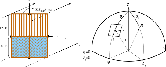
Figure 1: Left: Geometry of the 2D radiative transfer problem. The cartoon mimics the spatially inhomogeneous MHD atmosphere in the photosphere and horizontally homogeneous columns of FALC atmosphere in the chromosphere. The line $(X,Z_{\rm max})$ represents the surface where the radiation emerges from the 2D atmosphere. Right: The atmospheric reference frame. The angle pair $(\theta,\varphi)$ defines the outgoing ray direction. The magnetic field is characterized by $\bm{B}=(\Gamma,\theta_{B},\chi_{B})$, where $\Gamma$ is the Hanle efficiency parameter and ($\theta_{B},\chi_{B}$) defines the field direction. $\Theta$ is the scattering angle.

We consider an ellipse described by vibrations of an electric field vector corresponding to an elliptically polarized beam of light (see Chandrasekhar, 1960). Consider a plane transverse to the propagation direction of this beam of light in which we can decompose the specific intensity into components $I_{l}$ and $I_{r}$ along two mutually perpendicular directions $l$ and $r$ (see Figure 1, right panel). Then we define

$$I=I_{l}+I_{r},$$

$$Q=I_{l}-I_{r},$$

$$U=(I_{l}-I_{r})\tan 2\chi,$$ (1)

where $\chi$ is the angle between the semi-major axis of the ellipse and the direction $l$. Positive value of $Q$ is defined to be in a direction parallel to $l$ and negative $Q$ to be in a direction parallel to $r$. The vector $\bm{r}=({\rm x},{\rm y},{\rm z})$ denotes the position vector of the ray described by the direction cosines $\bm{\Omega}=(\eta,\gamma,\mu)=(\sin\theta\,\cos\varphi\,,\sin\theta\,\sin\varphi\,,\cos\theta)$ with respect to the atmospheric normal (the $Z$-axis in Figure 1, left panel). Here $\theta$ and $\varphi$ represent the polar and azimuthal angles of the ray (see Figure 1, right panel).

2.2 The cross-redistribution (XRD)

In this section we briefly describe the theoretical background of the XRD mechanism. For more details we refer the reader to Hubeny et al. (1983a, b) (see also Uitenbroek, 2001, and the references cited therein).

As described in Uitenbroek (2001), for a ray travelling in direction $\bm{\Omega}$, at wavelength $\lambda$, the emission profile coefficient denoted as $\psi$, in the case of a general XRD theory depends on the radiation field $I(\lambda,\bm{\Omega})$ in the line and its subordinate lines. It is given by

$$\left[\psi_{ij}(\lambda,\bm{\Omega})\right]_{\rm XRD}= \phi_{ij}(\lambda,\bm{\Omega})\Big{\{}1+\frac{\sum_{k<j}n_{k}B_{kj}}{n_{j}P_{j}}$$ (2)

$$\times\oint\frac{d\bm{\Omega}^{\prime}}{4\pi}\int d\lambda^{\prime}I(\lambda^{\prime},\bm{\Omega}^{\prime})\left[\frac{R_{kji}(\lambda,\bm{\Omega},\lambda^{\prime},\bm{\Omega}^{\prime})}{\phi_{ij}(\lambda,\bm{\Omega})}-\phi_{kj}(\lambda^{\prime},\bm{\Omega}^{\prime})\right]\Big{\}}.$$

In the case of ordinary PRD the summation over all subordinate lines in the emission profile coefficient reduces to just one term with $k=i$.

Here $n_{i},n_{j},n_{k}$ denote populations of $i,j,k$-th levels respectively; $R_{kji}$ are the cross-redistribution functions involving levels denoted by the subscripts $k$, $j$ and $i$; $\phi_{ij}$ denotes the Voigt profile function for the line corresponding to transition between levels $j$ and $i$; $B_{kj}$ or $B_{ji}$ being the Einstein-B coefficients for the transitions described by the subscripts $j$ and $i$; and $P_{j}$ denotes the sum of collisional and radiative rates, namely $P_{j}=\sum_{k\neq j}C_{jk}+R_{jk}$.

We note here that although general expressions given above can handle angle-dependent XRD/PRD problems, we restrict our attention in this paper to the angle-averaged redistribution functions (see Hummer, 1962).

3 Radiative transfer in the O i triplet

The method of solution used in this paper to compute the fractional linear polarization in the O i resonance line is the same as that explained in Anusha & Nagendra (2013, and references cited therein). For completeness we summarize the method briefly in this section.

In the first step we solve unpolarized transfer with the multi-level code of Uitenbroek (see Uitenbroek, 2001, hereafter called the RH code) with the O i model atom and a model atmosphere which is a combination of a two-dimensional (2D) snapshot of a three-dimensional (3D) magneto-hydrodynamical (MHD) atmosphere in the photosphere (see Nordlund & Stein, 1991), and columns of the one-dimensional FALC atmosphere in the chromosphere (see Fontenla et al., 1993). For the solution of unpolarized multi-level transfer equation with XRD the model atom used is the same as that used in Miller-Ricci & Uitenbroek (2002). It has 14 atomic energy levels with 18 line transitions and 13 continuum transitions in O i. A Grotrian diagram of the O i triplet and the other lines taken into account when solving with the RH-code is shown in Figure 2. The continuum transitions are not shown. The main lines of the triplet are results of the transitions ($3s\,\,^{3}S\rightarrow{2p^{4}}\,\,^{3}P_{0}$ : 1302.2 Å ), ($3s\,\,^{3}S\rightarrow{2p^{4}}\,\,^{3}P_{1}$ : 1304.9 Å ), and ($3s\,\,^{3}S\rightarrow{2p^{4}}\,\,^{3}P_{2}$ : 1306 Å ). The XRD theory of Hubeny et al. (1983a, b) is incorporated in the unpolarized transfer equation in the RH code. The RH-code computes radiative rates, collision rates, center-to-limb variation of the intensity spectrum $I(\lambda,\bm{\Omega})$ etc. in the O i triplet.

In the second step we only consider the resonance line (marked in bold in Figure 2), namely the line at 1302 Å , which is a result of the resonance transition $3s\,\,^{3}S\rightarrow{2p^{4}}\,\,^{3}P_{0}$. All the output parameters from the RH-code corresponding to this line are kept fixed in this step. For the fractional linear polarization computation in the second step, we adapt the irreducible spherical tensor notation (see e.g., Landi Degl’Innocenti & Landolfi, 2004; Frisch, 2007). We use $I(\lambda,\bm{\Omega})$ from the RH-code for both ordinary PRD and XRD cases as the initial unpolarized solution namely, the 6-component irreducible Stokes vector $\bm{\mathcal{I}}=(I^{0}_{0},0,0,0,0,0)^{T}$ (see e.g., Anusha & Nagendra, 2013). We then calculate the 6-component mean intensity vector in the two-level atom approximation with an unpolarized ground level given by

$$\bm{\mathcal{J}}(\lambda)=\frac{1}{\phi(\lambda)}\int_{-\infty}^{+\infty}d\lambda^{\prime}\oint\frac{d\bm{\Omega}^{\prime}}{4\pi}\hat{W}\Big{\{}\hat{M}_{\rm II}(\bm{B},\lambda,\lambda^{\prime})r_{\rm II}(\lambda,\lambda^{\prime})$$

$$+\hat{M}_{\rm III}(\bm{B},\lambda,\lambda^{\prime})r_{\rm III}(\lambda,\lambda^{\prime})\Big{\}}\hat{\Psi}(\bm{\Omega}^{\prime})\bm{\mathcal{I}}(\lambda^{\prime},\bm{\Omega}^{\prime}).$$ (3)

Here $\bm{B}$ represents an oriented magnetic field vector (see Figure 1, right panel). The matrix $\hat{\Psi}$ represents the reduced phase matrix for Rayleigh scattering. Its elements are listed in Appendix D of Anusha & Nagendra (2011b). The elements of the matrices $\hat{M}_{\rm II,III}(\bm{B},\lambda,\lambda^{\prime})$ for the Hanle effect are derived in Bommier (1997a, b). The functions $r_{\rm II}$ and $r_{\rm III}$ are the angle-averaged PRD functions of Hummer (1962), keeping the same notation as Anusha & Nagendra (2013). $\hat{W}$ is a diagonal matrix written as

$$\hat{W}=\textrm{diag}\{W_{0},W_{2},W_{2},W_{2},W_{2},W_{2}\},$$ (4)

with $W_{0}=1$. The angular momentum quantum number of the line under consideration determines the value of $W_{2}$ (see e.g., Landi Degl’Innocenti & Landolfi, 2004). For the O i line at 1302 Å , the factor $W_{2}=0.01$. Here $\phi(\lambda)$ represents the Voigt profile function for the resonance line at 1302 Å .

Computing the mean intensity vector is an important step in which linear polarization is generated from the unpolarized intensity vector. This step is the link between the multi-level atom unpolarized radiative transfer code (RH-code) and the two-level atom polarized radiative transfer code that computes linear polarization at 1302 Å . In this second step the polarization is generated iteratively similar to a perturbation process and we finally obtain converged fractional linear polarization. For more details on the computation of linear polarization we refer the reader to Anusha & Nagendra (2013, and the references cited therein). For future references we name the code used in the second step as POLY2D, which is a 2D extension of the so called POLY code developed by Fluri et al. (2003).

We note here that in this paper we use the word ‘XRD’ when we use cross redistribution theory in the RH-code to compute linear polarization using two-level atom PRD theory, and use the word ordinary ‘PRD’ when we use ordinary PRD theory in the RH code to compute linear polarization using two-level atom PRD theory.

4 Results and Discussions

In this section we present the intensity profiles of the O i triplet and linear polarization profiles of the O i line at 1302 Å  computed using the method described in Section 3. Our emphasis is on the fractional linear polarization spectrum of the O i line at 1302 Å . We also present an estimate of the errors in the resonance scattering fractional polarization, caused by not using XRD. We note here that the degree of the polarization in the O i resonance line is extremely small (because of the small $W_{2}$ factor), yet they are useful to theoretically predict the effects of XRD on the fractional linear polarization. All the results presented here correspond to a non-magnetic case ($\bm{B}=0$).

4.1 Intensity profiles

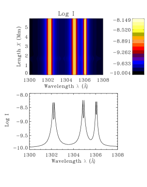
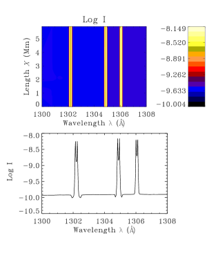
Figure 3: Top: The 2D spatial variation of the emergent, intensity profiles of the O i triplet line in log scale. Left panels are computed using ordinary PRD theory and those on the right panels are computed using XRD theory in the unpolarized multi-level radiative transfer. Bottom: Emergent, spatially averaged intensity profiles of the triplet in log scale.

In Figure 3 we show the emergent intensity profiles of the O i triplet in log scale computed from the 2D version of the RH-code for ordinary PRD and the XRD cases. We show both, namely the spatial variation of the emergent intensity profiles and their spatial averages. The color coding of the profiles in the top panels is shown in the corresponding color bars in each panel. The spatial homogeneity of the intensity profiles is caused by the fact that the formation height of the line core is in a region of the atmosphere where it is represented by the horizontally homogeneous FALC atmosphere. A comparison of the intensity profiles computed using the ordinary PRD and the XRD cases show similar conclusions as presented in Miller-Ricci & Uitenbroek (2002). The use of ordinary PRD instead of XRD leads to a broadening of the intensity profiles in the near-wings of the line. The reason is that, if we do not take XRD into account, the fraction of emissions that occur by excitation in two other lines of the triplet is counted as complete frequency redistribution (CRD) in the line under consideration, and clearly CRD leads to a broadening in the lines. Therefore assuming ordinary PRD decreases the coherency fraction of the lines.

4.2 Linear polarization profiles

In Figure 4 we present a spatial distribution of $(I/I_{\rm max},Q/I,U/I)$ profiles at the top of the 2D atmosphere for both the ordinary PRD and XRD cases. The color coding of the profiles is shown in the corresponding color bars in each panel. Clearly, differences between the ordinary PRD and XRD profiles are significant in both the line core and the near-wings of the line. Unlike the intensity profiles, the fractional linear polarization profiles are sensitive to the structuring in the atmosphere. The spatial variation due to inhomogeneities of the MHD atmosphere in the lower layers shows itself in the near-wings of the line which are formed in these layers (see Anusha & Nagendra, 2013). The spatial distribution of linear polarization shows significant differences between the ordinary PRD and XRD cases.

In Figure 5 we show the spatially averaged fractional polarization profiles $(I/I_{\rm max},Q/I,U/I)$ profiles where each of the Stokes parameters are spatially averaged before considering their ratios. These profile shapes are very much similar to the spatially averaged $(I,Q,U)$ profiles for the XRD and the ordinary PRD cases as shown in Figure 6. However in both these cases, the spatial averaging smears out large differences between XRD and the ordinary PRD fractional polarization profiles, which are clearly seen in Figure 4. This suggests that the differences between XRD and the ordinary PRD fractional polarization profiles become more significant in spatially resolved structures.

The 2D radiative transfer allows us to show the effects of XRD also in the resonance scattering values of $U/I$ - which is generated due to geometrical symmetry breaking in the medium.

In the case of scattering polarization, the quantities of interest have always been, the fractional polarization profiles. This is because of the following reasons. From the observational point of view, even in the most sophisticated polarimeter that measures scattering polarization to a very high accuracy, namely ZIMPOL (see e.g., Gandorfer et al., 2004), certain noise (seeing noise and gain table noise namely flat-field noise due to pixel-to-pixel sensitivity variations) in the observed data can be removed only by measuring the fractional polarization values $Q/I$ and $U/I$ at each wavelength point. The small values of $I$ in a given spectral region further makes it difficult to measure the polarization profiles $Q$ and $U$, because the latter are obtained through a decomposition of $I$ in two mutually perpendicular directions (see Equation 1 and Figure 6). From theoretical point of view, physically more meaningful are the fractional polarization profiles expressed in percents, in place of the $Q$ and $U$ profiles which are expressed in some arbitrary units.

For all these reasons, we conclude that the differences between XRD and ordinary PRD fractional polarization profiles need to be considered when modeling the observed fractional polarization signals.

4.3 Error estimation

As we discussed in the previous section, the XRD effects apparently become more visible in spatially resolved fractional polarization profiles (as seen in Figure 4), than in the spatially averaged case (as in Figures 5 and 6) as the latter smears out the differences. Therefore, to quantify the differences between ordinary PRD and XRD profiles in the spatially resolved case, we computed percent absolute error defined as

$$E=(|\,\,|X_{\textrm{XRD}}|-|X_{\textrm{P}RD}|\,\,|)\times 100,$$ (5)

where $X=(I/I_{\rm max},Q/I,U/I)$. We do not use the relative error because in some parts of the spectrum, values of the linear polarization approach zero in which case, errors become undefined.

In Figure 7 we show percent absolute error in $(I/I_{\rm max},Q/I,U/I)$, (in log scale), caused by using ordinary PRD theory instead of XRD theory. Due to steep gradient in the intensity profiles (see Figure 5), the errors can be as large as 28 % in the line wings ($\sim$1.44 in log scale) of intensity profiles. In $Q/I$ profiles, the maximum absolute error is 4 % ($\sim$ 0.62 in log scale) and in $U/I$, it is 2 % ($\sim$ 0.37 in log scale). These results clearly show that XRD can cause significant differences in intensity as well as linear polarization profiles, and needs to be used whenever possible and applicable.

On the one hand, the spatial distribution of the scattering polarization shows that it is sensitive to the structuring of the atmosphere. On the other hand significant differences between the spatial distribution of the polarization for the ordinary PRD and XRD cases show that whenever XRD is relevant, assumption of ordinary PRD may lead to significant errors. Therefore, the differences between ordinary PRD and XRD profiles is the outcome of both (1) multi-D transfer, and (2) the type of scattering theory used. In this way the XRD effects in combination with multi-D transfer are important to reproduce the amplitude and shapes of the observed scattering polarization profiles.

5 Conclusions

In this paper we have attempted to quantify for the first time, the effects of XRD on the fractional linear polarization using the example of the resonance line of O i triplet at 1302 Å . We use the anisotropy computed from the RH-code for both ordinary PRD and XRD theories, to compute the linear polarization based on the two-level atom PRD theory of Bommier (1997a, b). We present also an estimate of the percent absolute error when using the approximation of ordinary PRD theory instead of the more realistic XRD theory. This can be as large as 28 % for the intensity profiles, due to the steep gradients present in these profiles. In $Q/I$, the maximum error is 4 % and that in $U/I$ it is 2 %. We show a comparison of the spatial distribution of the fractional scattering polarization and the spatially averaged profiles for ordinary PRD and XRD cases. We conclude that the fractional linear polarization signals are sensitive to the structuring of the atmosphere and that the XRD effects become more significant in spatially resolved cases than in the spatially averaged case as the latter smears out the large differences. Therefore, to reproduce the amplitude and shape of observed scattering polarization signals of the O i line at 1302 Å , a multi-dimensional radiative transfer including XRD theory is important.

Figure 2: Grotrian diagram of the O i triplet showing all the eighteen line transitions that are taken into account in the unpolarized radiative transfer calculations in the RH-code. The 1300 triplet line transitions are labelled with the line center wavelengths. The energy levels of the resonance line transition at 1302.2 Å  are marked in bold lines the diagram.

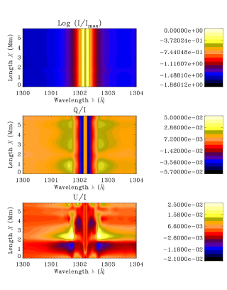
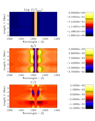
Figure 4: Spatial distribution of $(I/I_{\rm max},Q/I,U/I)$ for the first direction in Carlsson A4 angular grid Carlsson (1963), namely, $(\mu,\varphi)=(0.3,160^{\circ})$ on the top of the 2D atmosphere. Left panels are computed using ordinary PRD theory and those on the right panels are computed using XRD theory in the unpolarized multi-level radiative transfer.

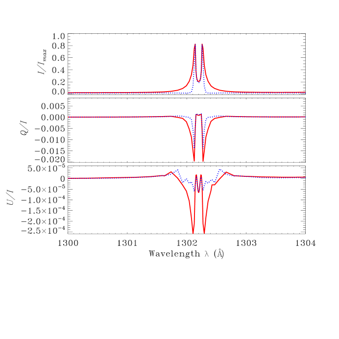
Figure 5: $(I/I_{\rm max},Q/I,U/I)$ profiles with each of the Stokes parameters spatially averaged, for ordinary PRD (solid red curves) and XRD (dotted blue curves) cases for $(\mu,\varphi)=(0.3,160^{\circ})$.

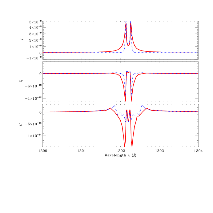
Figure 6: Spatially averaged $(I,Q,U)$ profiles for ordinary PRD (solid red curves) and XRD (dotted blue curves) cases for $(\mu,\varphi)=(0.3,160^{\circ})$.

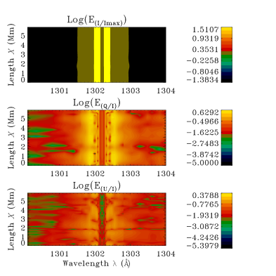
Figure 7: Percent absolute errors in $(I/I_{\rm max},Q/I,U/I)$ profiles, expressed in log scale, computed using Equation (5) for $(\mu,\varphi)=(0.3,160^{\circ})$.

References

- Anusha & Nagendra (2011b) Anusha, L. S., & Nagendra, K. N. 2011b, ApJ, 738, 116
- Anusha & Nagendra (2013) Anusha, L. S., & Nagendra, K. N. 2013, ApJ, 767, 108
- Anusha et al. (2010) Anusha, L. S., Nagendra, K. N., Stenflo, J. O., Bianda, M., Sampoorna, M., Frisch, H., Holzreuter, R., & Ramelli, R. 2010, ApJ, 718, 988
- Bommier (1997a) Bommier, V. 1997a, A&A, 328, 706
- Bommier (1997b) Bommier, V. 1997b, A&A, 328, 726
- Bommier (2003) Bommier, V. 2003, in Solar Polarization, ed. J. Trujillo Bueno & J. Sánchez Almeida (San Francisco: ASP), 213
- Carlsson (1963) Carlsson, B. G. 1963, in Methods in Computational Physics, Vol 1, Academic Press, 1
- Carlsson & Judge (1993) Carlsson, M.; Judge, P. G. 1993, ApJ, 402,344
- Chandrasekhar (1960) Chandrasekhar, S. 1960, Radiative Transfer (New York: Dover)
- Fontenla et al. (1993) Fontenla, J. M., Avrett, E. H., & Loeser, R. 1993, ApJ, 406, 319
- Frisch (2007) Frisch, H. 2007, A&A, 476, 665
- Gandorfer et al. (2004) Gandorfer, A. M., Povel H. P., Steiner, P., Aebersold, F., Egger, U.,
- Landi Degl’Innocenti & Landolfi (2004) Landi Degl’Innocenti, E., & Landolfi, M. 2004, Polarization in Spectral Lines (Dordrecht: Kluwer)
- Miller-Ricci & Uitenbroek (2002) Miller-Ricci, E. & Uitenbroek, H. 2002, ApJ, 566, 500
- Nordlund & Stein (1991) Nordlund, Å ., & Stein, R. F., 1991, in Stellar Atmospheres: Beyond Classical Models, NATO ASI Series C, 341, ed. L. Crivellari, I. Hubeny, & D. G. Hummer (Dordrecht: Kluwer), 263
- Hubeny et al. (1983a) Hubeny, I., Oxenius, J., & Simonneau, E. 1983a, JQSRT, 29, 477
- Hubeny et al. (1983b) Hubeny, I., Oxenius, J., & Simonneau, E. 1983a, JQSRT, 29, 495
- Hummer (1962) Hummer, D. G. 1962, MNRAS, 125, 21
- Fluri et al. (2003) Fluri, D. M., Holzreuter, R., Klement, J., & Stenflo, J. O. 2003, in ASP Conf. Ser. 307, Solar Polarization III, ed. J. Trujillo-Bueno & J. Sanchez Almeida (San Francisco, CA: ASP), 227
- Sampoorna et al. (2013) Sampoorna, M., Nagendra, K. N. & Stenflo, J. O. 2013, ApJ, 770, 92
- Uitenbroek (2001) Uitenbroek, H. 2001, ApJ, 557, 389