Coupled Vlasov and two-fluid codes on GPUs

Abstract

We present a way to combine Vlasov and two-fluid codes for the simulation of a collisionless plasma in large domains while keeping full information of the velocity distribution in localized areas of interest. This is made possible by solving the full Vlasov equation in one region while the remaining area is treated by a 5-moment two-fluid code. In such a treatment, the main challenge of coupling kinetic and fluid descriptions is the interchange of physically correct boundary conditions between the different plasma models. In contrast to other treatments, we do not rely on any specific form of the distribution function, e.g. a Maxwellian type. Instead, we combine an extrapolation of the distribution function and a correction of the moments based on the fluid data. Thus, throughout the simulation both codes provide the necessary boundary conditions for each other. A speed-up factor of around 20 is achieved by using GPUs for the computationally expensive solution of the Vlasov equation and an overall factor of at least 60 using the coupling strategy combined with the GPU computation. The coupled codes were then tested on the GEM reconnection challenge.

1 Introduction

For many relevant problems in plasma physics, the plasma can be considered non-collisional or even collisionless. In these cases, the Vlasov-Maxwell system is sufficient for a complete description of the physically important phenomena. Nevertheless, it is close to impossible to numerically solve the Vlasov equation for global problems on fluid scales due to the vast amount of memory needed to resolve a 6-dimensional phase-space. However, in many situations a complete kinetic description is not necessary and computationally inexpensive fluid models based on the moments of the distribution function are sufficient. In addition, plasmas are typical multi-scale phenomena. Often there are only localized and small regions, where a kinetic description is needed, whereas the rest of the domain can be described by means of a fluid model. This separation of scales can be found in many typical problems of plasma physics, such as reconnection in the magnetotail of the earth, solar flares or typical phenomena in tokamaks. To determine what amount of computational savings coupling techniques might provide, a rough estimation of the numerical costs can be made on the basis of spatial scales. To do this, both the computational effort for the fluid region and the overhead for the coupling itself can be assumed as negligible compared to the costs of the kinetic part of the simulation. Thus the fraction of the domain where kinetic effects occur can indicate how much computational time might be saved. This fraction can be estimated on the basis of typical plasma parameters. The most relevant scales are determined by the ion skin depth, below which the dynamics of ions and electrons decouple, and the ion gyro radius, which is especially important in the context of non-collisional plasmas.

In the magnetotail of the earth, kinetic effects are important in and around the current sheet, where reconnection takes place. In an example of a typical setup for this problem given by Birn et al. [1], the current sheet–and thus the kinetic region–covers around 10% of the computational domain. In a typical tokamak with an overall size $\sim 1\,\mathrm{m}$, the ion skin depth is $\sim 5\,\mathrm{cm}$ (see Woods [2]). The ion gyro radius is even one order of magnitude smaller. Thus, taking into account the rotationally symmetric geometry of a tokamak and the magnetic field therein, the fraction of the domain where localized kinetic effects as reconnection might take place is likely to scale with the fraction of $5\,\mathrm{cm}/1\,\mathrm{m}$ and can thus be expected to be only 5% of the domain, to give a very rough estimation of the order of magnitude. In a solar flare, the ratio is even smaller: A typical size of $\sim 10^{7}\,\mathrm{m}$ compares to an ion skin depth of about $10\,\mathrm{m}$ (see for example Ramesh et al. [3]).

If the kinetic regions are known, this additional information might be used to reduce the computational costs drastically by restricting the expensive kinetic simulation to this smaller area and using a suitable fluid model for the rest of the domain. There have been several approaches to exploit this ansatz in numerical schemes. In the works of Degond et al. [4], Dellacherie [5], Goudon et al. [6], Klar et al. [7], and Le Tallec and Mallinger [8] methods for coupling the Boltzmann equation to some kind of fluid model like the Navier-Stokes or Euler-equations are adressed. Sugiyama and Kusano [9] describe the coupling of PIC and MHD models, Markidis et al. [10] show a way to combine PIC and fluid models, and Kolobov and Arslanbekov [11] describe the transition from neutral gas models to models of weakly ionized plasmas with respect to coupling kinetic and fluid equations. Schulze et al. [12] use coupling techniques in the context of epitaxial growth.

Most of these schemes are based on the strong assumption that the distribution function is close to Maxwellian in the vicinity of the coupling border and use this approximation to generate boundary conditions for the kinetic region. In other approaches, an artificial field is introduced that expresses the deviation from a Maxwellian and is coupled to the underlying equations [4], or the fluxes at the boundary are used for the coupling [8].

This paper presents a different mechanism for coupling the Vlasov equation with a five-moment model and the full Maxwell equations. Our method is easy to implement and does not rely on any specific assumptions with respect to the distribution function near the coupling border. In addition, no extensive transition region between the kinetic and fluid domains is required.

The rest of this paper is organized as follows: After the physical models have been described in Sec. 2, the numerical schemes are presented in Sec. 3. The coupling procedure is explained in Sec. 4. Finally, in Sections 5 and 6, first numerical results are presented and discussed.

2 Physical models

Consider a plasma consisting of different particle species $s$. The Vlasov equation

$$\partial_{t}f_{s}+\textbf{v}\cdot\nabla_{\textbf{x}}f_{s}+\frac{q_{s}}{m_{s}}(\textbf{E}+\textbf{v}\times\textbf{B})\cdot\nabla_{\textbf{v}}f_{s}=0$$ (1)

describes the time evolution of the phase-space density $f_{s}(\textbf{x},\textbf{v},t)$, where E is the electric field, B is the magnetic field, $q_{s}$ is the charge, and $m_{s}$ is the mass per particle. By calculating the moments of $f_{s}$ with respect to v, we can derive important physical quantities describing the plasma:

the mass density $$\rho_{s} =m_{s}\int f_{s}\mathrm{d}^{3}v,$$ (2)

the momentum density $$\textbf{u}_{s} =m_{s}\int\textbf{v}f_{s}\mathrm{d}^{3}v,$$ (3)

and the energy density $$\mathcal{E}_{s} =\frac{m_{s}}{2}\int\textbf{v}^{2}f_{s}\mathrm{d}^{3}v.$$ (4)

Their time dependence can be calculated from the Vlasov equation (1) and is given by:

$$\partial_{t}\rho_{s} =-\nabla\cdot\textbf{u}_{s}$$ (5)

$$\partial_{t}\textbf{u}_{s} =-\nabla\cdot\left(\frac{\textbf{u}_{s}\otimes\textbf{u}_{s}}{\rho_{s}}+\mathbb{P}_{s}\right)+\frac{q_{s}}{m_{s}}(\rho_{s}\textbf{E}+\textbf{u}_{s}\times\textbf{B}_{s})$$ (6)

$$\partial_{t}\mathcal{E}_{s} =-\nabla\cdot\left(\frac{\mathcal{E}_{s}\mathds{1}+\mathbb{P}_{s}}{\rho_{s}}\textbf{u}_{s}\right)-\nabla\cdot\textbf{Q}_{s}+\frac{q_{s}}{m_{s}}\textbf{u}_{s}\cdot\textbf{E},$$ (7)

where $\mathbb{P}_{s}$ is the pressure tensor, $3p_{s}=\mathrm{Tr}\;\mathbb{P}_{s}$ is the trace of the pressure tensor, and $\textbf{Q}_{s}$ is the heat flux tensor. These quantities must be provided in order to close the system.

For our first tests of the coupling procedure, we assume that the plasma is adiabatic and the pressure to be isotropic, which corresponds to

$$\mathbb{P}_{s}=p_{s}\mathds{1},\hskip 10.00002ptp_{s}=\frac{2}{3}\mathcal{E}_{s}-\frac{1}{3}\frac{\textbf{u}_{s}^{2}}{\rho_{s}},\hskip 10.00002pt\text{and}\hskip 10.00002pt\nabla\cdot\textbf{Q}_{s}=0$$ (8)

respectively. Note that this fluid closure was chosen for simplicity and other fluid models may be used depending on the situation of the plasma application.

Furthermore Faraday’s and Ampère’s laws

$$\partial_{t}\textbf{B} =-\nabla\times\textbf{E}$$ (9)

$$\partial_{t}\textbf{E} =c^{2}(\nabla\times\textbf{B}-\mu_{0}\textbf{j})$$ (10)

are required to determine how the electromagnetic fields evolve where current density j is given by

$$\textbf{j}=\sum_{s}\frac{q_{s}}{m_{s}}\textbf{u}_{s}.$$ (11)

3 Numerical schemes

In order to solve the coupling problem, we must first design numerical schemes for solving the Vlasov equation, the five-moment two-fluid equations and the Maxwell equations separately. It is important to note that we have chosen the fluid model with care such that we do not impose a generalized Ohm’s law to obtain the electric field E but use the same set of Maxwell equations as for the Vlasov equations. This implies that timescales of both fluid and kinetic descriptions are comparable. This allows for a clean separation between the Maxwell solver, the Vlasov solver and the fluid solver. That is, the Maxwell solver only requires the current density as a source term, which can be obtained from the fluid and the Vlasov solver.

Coupling to even larger spatial and temporal scales which could be described with an MHD model, would thus be more related to the question of coupling Maxwell’s equation to a generalized Ohm’s law. This kind of coupling can be done on the fluid level (2-fluid with Maxwell-equation coupled to MHD with generalized Ohm’s law). This is still a major task and will be the next necessary step.

Both models, the Vlasov equation and the two-fluid equations, are implemented numerically and each code can be executed alone or coupled to the other—a concept known as multiple program multiple data (MPMD).

Because of the high dimensionality of the distribution function $f_{s}$, the Vlasov code is much more computationally expensive than the fluid code. Therefore, to achive optimal performance, the Vlasov code is executed on multiple GPUs, while the relatively low cost fluid model and Maxwell’s equations (9) and (10) are solved on CPUs. The network communication is implemented via OpenMPI. Our code solves the 2.5-dimensional problem (i.e. two space dimensions and three velocity dimensions), but a generalisation to the full 3-dimensional case is straightforward. In the following subsections we will describe the numerical schemes. In addition to that, a detailed description of semi-Lagrangian solvers is given because they are essential both to the Vlasov code and to the coupling routine that will be explained in section 4.

3.1 Numerical implementation of the Vlasov equation

In this section, the numerical solver for the Vlasov equation used in this work is described. By means of splitting methods, the Vlasov equation is broken down into a set of simpler one-dimensional conservation laws. These can then be solved with a semi-Lagrangian scheme. Such a scheme requires finding the characteristics for which we use the Backsubstitution method, and approximating the integrals between these characteristics, which we do by means of the PFC scheme.

3.1.1 Conservative semi-Lagrangian schemes

The underlying idea of how to solve conservation laws by means of semi-Lagrangian schemes is now described. As an example consider

$$\partial_{t}f(x,t)+\partial_{x}\big{(}u(x,t)f(x,t)\big{)}=0.$$ (12)

Let the domain be divided into equal cells and the $i^{\mathrm{th}}$ cell be bounded by the points $x_{i}$ and $x_{i+1}$. Different points in time, separated by the time interval $\Delta t$, are denoted as $t^{n}=n\Delta t$. The scheme will then evolve the cell integrals

$$\overline{f_{i}}(t^{n})=\int_{{x_{i}}}^{{x_{i+1}}}f(x,t^{n})\,\mathrm{d}x$$ (13)

in time. Next, a family of curves $\mathcal{C}(t;x,s)$ is introduced, called the characteristics of equation (12), which are defined by

$$\frac{\mathrm{d}}{\mathrm{d}t}\mathcal{C}(t) =u(\mathcal{C}(t),t)$$ (14)

$$\mathcal{C}(t=s) =x.$$ (15)

Integrating $f$ along $x$ between the two curves that pass through the cell boundaries of cell $i$ at time $t^{n+1}$, taking the time derivative, using the chain rule for parameter integrals, and inserting the conservation law (12) leads to

$$\frac{\mathrm{d}}{\mathrm{d}t}\int_{{\mathcal{C}(t;x_{i},t^{n+1})}}^{{\mathcal{C}(t;x_{i+1},t^{n+1})}}f(x,t)\,\mathrm{d}x=0.$$ (16)

If the velocity field $u(x,t)$ is Lipschitz continuous, the Picard-Lindelöf theorem will guarantee that two different characteristics will never intersect. Then we may integrate over time to obtain

$$\overline{f_{i}}(t^{n+1})=\int_{{\mathcal{C}(t^{n};x_{i},t^{n+1})}}^{{\mathcal{C}(t^{n};x_{i+1},t^{n+1})}}f(x,t^{n})\,\mathrm{d}x.$$ (17)

Where $\overline{f_{i}}(t^{n})$ and the points $\mathcal{C}(t^{n};x_{i},t^{n+1})$ are known, the cell integrals $\overline{f_{i}}(t^{n+1})$ can be found by reconstructing the right hand side of equation (17) from the $\overline{f_{i}}(t^{n})$ by means of an arbitrary reconstruction scheme. In other words, in order to solve the conservation law (12), it is sufficient to find the source points of the characteristics that will pass through the cell boundaries.

3.1.2 Splitting

The phase space density $f_{S}$ depends on six coordinates plus time. Trying to solve the Vlasov equation in a naive way by simply discretizing it based on an arbitrary scheme would lead to severe problems: If the number of dimensions is $d$, the number of direct neighbours of a given cell is $3^{d}-1$. Even if one spatial dimension can be left out because of the symmetry of the problem, this still results in 242 cells. A stencil spanning a larger part of these cells, would produce a very clumsy and slow scheme. This exponential growth of the number of dependencies can be avoided by splitting the Vlasov equation into smaller parts that are more manageable and can be solved separately. If this is done carefully, the resulting error does not exceed the one of the overall scheme.

The Vlasov equation can be written in the form

$$\partial_{t}f_{s}+(\mathcal{A}+\mathcal{B})f_{s}=0$$ (18)

with operators

$$\mathcal{A}=\textbf{v}\cdot\nabla_{\textbf{x}}$$

and

$$\mathcal{B}=\frac{q_{s}}{m_{s}}(\textbf{E}+\textbf{v}\times\textbf{B})\cdot\nabla_{\textbf{v}}.$$

Instead of solving the full equation (18), we consider the equations

$$\partial_{t}f_{s}+\mathcal{A}f_{s}=\partial_{t}f_{s}+\textbf{v}\cdot\nabla_{\textbf{x}}f_{s}=0$$ (19)

and

$$\partial_{t}f_{s}+\mathcal{B}f_{s}=\partial_{t}f_{s}+\frac{q_{s}}{m_{s}}(\textbf{E}+\textbf{v}\times\textbf{B})\cdot\nabla_{\textbf{v}}f_{s}=0.$$ (20)

Now, given some differential equation

$$\partial_{t}f+\mathcal{S}f=0,\quad f(t=0)=f_{0}$$ (21)

we can write its formal solution as $f(\Delta t)=\exp(-\Delta t\mathcal{S})f_{0}=:T(\mathcal{S})f_{0}$.

With this notation in mind we can decompose the solution of (18) in terms of solutions of (19) and (20) by making use of the Strang splitting method:

$$f_{s}(t+\Delta t)=T(\mathcal{A}+\mathcal{B})f(t)=T\left(\frac{1}{2}\mathcal{A}\right)T(\mathcal{B})T\left(\frac{1}{2}\mathcal{A}\right)f(t)+\mathcal{O}(\Delta t^{3}).$$ (22)

This decomposition is exact if the operators $\mathcal{A}$ and $\mathcal{B}$ commute. However, this is not the case here, but the resulting error is of third order in time and thus does not destroy the overall accuracy. Now that the problem has been split into two subproblems, each one can be solved separately. In both (19) and (20) the operators still act on a three-dimensional space. It is natural to try to decompose the operators $\mathcal{A}$ and $\mathcal{B}$ further in order to simplify the problem even more and make it possible to solve it with a semi-Lagrangian scheme which only works for one dimension. As for $\mathcal{A}$, which is the sum of three commuting operators, this splitting is exact and can easily be done by a simple composition of the single operators.

The operator $\mathcal{B}$, however, does not allow for such an easy decomposition. Here, it would be possible to use Strang splitting again, but there would be some disadvantages in this. First, the resulting scheme would be non-isotropic, as the single operators would not be used the same number of times. Second, the application of these operators is particularly expensive, so it is not desirable to apply them no more than necessary.

Thus, the next problem is to find a splitting so that equation (20) can be solved by only three applications of the time-evolution operator (one for each dimension of v) and obtain at least second-order accuracy in space and time. We rewrite (20) as

$$\partial_{t}f_{s}+\mathcal{B}f_{s}=\partial_{t}f_{s}+(\mathcal{V}_{x}+\mathcal{V}_{y}+\mathcal{V}_{z})f_{s}=0$$ (23)

with

$$\mathcal{V}_{i}=\frac{q_{s}}{m_{s}}(E_{i}+(\textbf{v}\times\textbf{B})_{i})\partial_{i}$$

and make the ansatz

$$f(t+\Delta t)=T(\tilde{\mathcal{V}}_{z})T(\tilde{\mathcal{V}}_{y})T(\tilde{\mathcal{V}}_{x})f(t)+E_{\mathrm{split}}+E_{\mathrm{mod}}.$$ (24)

with modified operators $\tilde{\mathcal{V}}_{i}$ that still have to be determined. The term $E_{\mathrm{split}}$ represents the error due to the splitting scheme, while $E_{\mathrm{mod}}$ is the error caused by modifying the operators. If the modifications are chosen correctly, both error terms cancel out and the splitting is exact. It should be noted however, that the error term of the splitting depends on the order in which the solution operators are applied. Thus it is not possible to change the order of execution of the $T(\tilde{\mathcal{V}}_{i})$ once the modifications have been chosen. The implementation of (24) is done by means of the Backsubstitution method, which is described in the next section.

3.1.3 The Backsubstitution Method

The Backsubstitution method [13, 14] relies on the calculation of the characteristics needed for the semi-Lagrangian schemes that occur in the single operators in (24) by means of the Boris push method. The latter is best known from the context of PIC simulations.

We start with a review of the Boris push method. Considering the discretized equation

$$\frac{\textbf{v}^{n+1}-\textbf{v}^{n}}{\Delta t}=\frac{q_{\alpha}}{m_{\alpha}}\left(\textbf{E}^{n+1/2}+\frac{\textbf{v}^{n+1}+\textbf{v}^{n}}{2}\times\textbf{B}^{n+1/2}\right),$$ (25)

the effects of the electric and magnetic fields can be separated by introducing new variables

$$\textbf{v}^{+}=\textbf{v}^{n+1}-\frac{q_{\alpha}}{m_{\alpha}}\frac{\Delta t}{2}\textbf{E}^{n+1/2}\hskip 28.45274pt\mathrm{and}\hskip 28.45274pt\textbf{v}^{-}=\textbf{v}^{n}+\frac{q_{\alpha}}{m_{\alpha}}\frac{\Delta t}{2}\textbf{E}^{n+1/2}.$$ (26)

With that, equation (25) becomes

$$\frac{\textbf{v}^{+}-\textbf{v}^{-}}{\Delta t}=\frac{q_{\alpha}}{m_{\alpha}}\frac{\textbf{v}^{+}+\textbf{v}^{-}}{2}\times\textbf{B}^{n+1/2}.$$ (27)

This equation is solved in two steps. Introducing the quantities

$$\textbf{t}=\frac{q_{\alpha}}{m_{\alpha}}\frac{\Delta t}{2}\textbf{B}\hskip 28.45274pt\mathrm{and}\hskip 28.45274pt\textbf{s}=\frac{2\textbf{t}}{1+t^{2}},$$ (28)

the first step calculates an intermediate vector $\textbf{v}^{\prime}$ from $\textbf{v}^{-}$, the second step uses this intermediate vector to calculate the result $\textbf{v}^{+}$

$$\textbf{v}^{\prime} =\textbf{v}^{-}+\textbf{v}^{-}\times\textbf{t}$$ (29)

$$\textbf{v}^{+} =\textbf{v}^{-}+\textbf{v}^{\prime}\times\textbf{s}$$ (30)

There is also a backward-in-time version of the Boris push that calculates $\textbf{v}^{-}$ from $\textbf{v}^{+}$:

$$\widetilde{\textbf{v}}^{\prime} =\textbf{v}^{+}-\textbf{v}^{+}\times\textbf{t}$$ (31)

$$\textbf{v}^{-} =\textbf{v}^{+}-\widetilde{\textbf{v}}^{\prime}\times\textbf{s}.$$ (32)

A big advantage of the Boris push is that it correctly conserves energy respectively the length of v if only magnetic and no electric fields are present.

Following the idea of cascade interpolation [15], the first step of the update in velocity space will be performed along the $\textbf{v}_{x}$ direction, the second step along $\textbf{v}_{y}$, and the last step along $\textbf{v}_{z}$. For the last step, the distance along the $\textbf{v}_{z}$ direction is just the $z$ component of the characteristic ending exactly at the grid point. Since we are tracing the characteristics back in time, the grid-point coordinates are denoted by $\textbf{v}^{n+1}$. By using the new variables (26), the electric fields can be removed from the equations and the grid-point coordinates become $\textbf{v}^{+}$. The distance for the $\textbf{v}_{z}$ update is then given by a formula $v^{-}_{z}=v^{-}_{z}(v^{+}_{x},v^{+}_{y},v^{+}_{z})$. This notation means that $v_{z}^{-}$ is a function of the variables $v^{+}_{x}$, $v^{+}_{y}$, and $v^{+}_{z}$. Using the $z$ component of equations (31) and (32), one obtains

$$v_{z}^{-}=v_{x}^{+}(t_{z}s_{x}-s_{y})+v_{y}^{+}(t_{z}s_{y}+s_{x})+v_{z}^{+}(1-t_{x}s_{x}-t_{y}s_{y})$$ (33)

for the sought-after function. The step along the $\textbf{v}_{y}$ direction follows a characteristic passing through $v_{z}^{+}$ at time $t-\Delta t$ and $v_{y}^{+}$ and $v_{x}^{+}$ at time $t$. This means that an equation of the form $v_{y}^{-}=v_{y}^{-}(v_{x}^{+},v_{y}^{+},v_{z}^{-})$ is needed. This can be obtained by solving Eq. (33) for $v_{z}^{+}$ and inserting the result into the $y$ component of equation (32), yielding

$$v_{y}^{-} =v_{x}^{+}\left(s_{x}t_{y}+s_{z}-\frac{(t_{z}s_{x}-s_{y})(t_{y}s_{z}-s_{x})}{1-t_{x}s_{x}-t_{y}s_{y}}\right)$$ (34)

$$\;\;\;+v_{y}^{+}\left(1-t_{x}s_{x}-t_{z}s_{z}-\frac{(t_{z}s_{y}+s_{x})(t_{y}s_{z}-s_{x})}{1-t_{x}s_{x}-t_{y}s_{y}}\right)$$

$$\;\;\;+v_{z}^{-}\frac{t_{y}s_{z}-s_{x}}{1-t_{x}s_{x}-t_{y}s_{y}}.$$

For the last step, the equation for $v_{z}^{-}$ has the form $v_{z}^{-}=v_{z}^{-}(v_{x}^{+},v_{y}^{-},v_{z}^{-})$. In the original version of the backsubstitution method [13], this equation was obtained in a similar way by solving Eqs. (33) and (34) for $v_{z}^{+}$ and $v_{y}^{+}$, respectively, and “substituting them back” into the $x$ component of equation (32). However, this results in a lengthy calculation, and it is difficult to simplify the resulting expression. There is an easier way to obtain the final result using the forward-in-time version of the Boris push and solving the $x$ component of equation (30) for $v_{x}^{-}$, which results in

$$v_{x}^{-}=\frac{v_{x}^{+}-v_{y}^{-}(t_{x}s_{y}+s_{z})-v_{z}^{-}(t_{x}s_{z}-s_{y})}{1-t_{y}s_{y}-t_{z}s_{z}}.$$ (35)

Equations (35), (34), and (33) provide the starting points for the one-dimensional updates along the $\textbf{v}_{x}$, $\textbf{v}_{y}$, and $\textbf{v}_{z}$-axis, respectively. The order in which these steps must be applied is $\textbf{v}_{x}$, then $\textbf{v}_{y}$, then $\textbf{v}_{z}$.

3.1.4 The PFC Scheme

In this section we present a brief review of the positive flux-conservative (PFC) scheme developed by Filbet et al. [16], which is used in this work and provides a method for calculating the integral in Eq. (17). For a comparison of other schemes that might be used for the same purpose, see Crouseilles et al. [17].

The PFC scheme is used to approximate the function $f$ on the basis of its cell integral $f_{i}$ in the $i^{\mathrm{th}}$ cell. Here, the case of a positive velocity $u$ is discussed. The case $u<0$ can be derived analogously. From Eq. (17) it holds that

$${f_{i}^{n}}=\int_{x_{i-1/2}}^{x_{i+1/2}}f(x,t^{n})\mathrm{d}x=\int_{{X(t^{n-1};x_{i-1/2},t^{n})}}^{{X(t^{n-1};x_{i+1/2},t^{n})}}f(x,t^{n-1})\mathrm{d}x.$$ (36)

By setting

$$\Phi_{i+1/2}=\int_{{X(t^{n-1};x_{i+1/2},t^{n})}}^{{x_{i+1/2}}}f(x,t^{n-1})\mathrm{d}x,$$ (37)

equation (36) can be rewritten as an update equation for the $f_{i}$:

$$f_{i}^{n}=f_{i}^{n-1}+\Phi_{i-1/2}-\Phi_{i+1/2}.$$ (38)

The primitive function of $f$ at the cell borders is given by

$$F(t^{n},x_{k-1/2})=\sum_{i=0}^{k-1}f_{i}^{n}.$$ (39)

An approximation $\widetilde{F}$ of $F$ within the $i^{\mathrm{th}}$ cell can be obtained by Newton interpolation of $F$ on the cell borders $\{x_{i-3/2},x_{i-1/2},x_{i+1/2},x_{i+3/2}\}$:

$$\widetilde{F}(x)=\; F(x_{i-3/2})+f_{i-1}(x-x_{i-3/2})+\frac{f_{i}-f_{i-1}}{2\Delta x}(x-x_{i-3/2})(x-x_{i-1/2})$$ (40)

$$+\frac{f_{i+1}-2f_{i}+f_{i-1}}{6(\Delta x)^{2}}(x-x_{i-3/2})(x-x_{i-1/2})(x-x_{i+1/2})$$

By differentiating and rearranging the terms, one obtains an approximation $\widetilde{f}$ in the $i^{\mathrm{th}}$ cell:

$$\widetilde{f}(x) =\frac{\mathrm{d}\widetilde{F}(x)}{\mathrm{d}x}(x)$$ (41)

$$=f_{i}+\frac{f_{i+1}-f_{i}}{6(\Delta x)^{2}}\big{(}2(x-x_{i})(x-x_{i-3/2})+(x-x_{i-1/2})(x-x_{i+1/2})\big{)}$$ (42)

$$\hskip 9.00002pt+\frac{f_{i}-f_{i-1}}{6(\Delta x)^{2}}\big{(}2(x-x_{i})(x-x_{i+3/2})+(x-x_{i-1/2})(x-x_{i+1/2})\big{)}$$

This reconstruction can create negative values of $\widetilde{f}(x)$, or values larger than $f_{\infty}=\max(f(x))$, which would be an unphysical solution to the Vlasov equation. Thus, slope limiters are introduced:

$$\epsilon_{i}^{+} =\begin{cases}\min(1;2f_{i}/(f_{i+1}-f_{i}))&\mathrm{if\;}f_{i+1}>f_{i}\\ \min(1;-2(f_{\infty}-f_{i})/(f_{i+1}-f_{i}))&\mathrm{if\;}f_{i+1}<f_{i}\end{cases}$$ (43)

$$\epsilon_{i}^{-} =\begin{cases}\min(1;2(f_{\infty}-f_{i})/(f_{i}-f_{i-1}))&\mathrm{if\;}f_{i}>f_{i-1}\\ \min(1;-2f_{i}/(f_{i}-f_{i-1}))&\mathrm{if\;}f_{i}<f_{i-1},\end{cases}$$ (44)

and the approximation becomes

$$\widehat{f}_{i}(x)=f_{i} +\epsilon_{i}^{+}\frac{f_{i+1}-f_{i}}{6(\Delta x)^{2}}\big{(}2(x-x_{i})(x-x_{i-3/2})+(x-x_{i-1/2})(x-x_{i+1/2})\big{)}$$ (45)

$$+\epsilon_{i}^{-}\frac{f_{i}-f_{i-1}}{6(\Delta x)^{2}}\big{(}2(x-x_{i})(x-x_{i+3/2})+(x-x_{i-1/2})(x-x_{i+1/2})\big{)}.$$

The flux $\Phi_{i+1/2}$ can be approximated by integrating $\widehat{f}_{i}(x)$ from $X(t^{n-1};x_{i+1/2},t^{n})$ to $x_{i+1/2}$ (see equation (37)). It was assumed that the velocity $u$ used in calculating the characteristic $X$ is positive. Because the characteristic is followed backwards in time, its footpoint lies to the left of $x_{i+1/2}$. However, due to the semi-Lagrangian nature of this scheme, the point $X(t^{n-1};x_{i+1/2},t^{n})$ might not be located in the $i^{\mathrm{th}}$ cell, but multiple cells further to the left. Setting $j$ so that $X(t^{n-1};x_{i+1/2},t^{n})$ lies in the $j^{\mathrm{th}}$ cell and defining $\alpha_{i}=(x_{j+1/2}-X(t^{n-1};x_{i+1/2},t^{n}))/\Delta x$ one obtains

$$\Phi_{i+1/2}=\sum_{k=j+1}^{i}f_{k}+\alpha_{i}\left(\vphantom{\frac{\epsilon_{j}^{+}}{6}}f_{j}\right. +\frac{\epsilon_{j}^{+}}{6}(1-\alpha_{i})(2-\alpha_{i})(f_{j+1}-f_{j})$$ (46)

$$+\left.\frac{\epsilon_{j}^{-}}{6}(1-\alpha_{i})(1+\alpha_{i})(f_{j}-f_{j-1})\right).$$

For negative velocities, $\alpha_{i}=(x_{j-1/2}-X(t^{n-1};x_{i+1/2},t^{n}))/\Delta x$ can be used in

$$\Phi_{i+1/2}=-\sum_{k=j+1}^{i}f_{k}+\alpha_{i}\left(\vphantom{\frac{\epsilon_{j}^{+}}{6}}f_{j}\right. -\frac{\epsilon_{j}^{+}}{6}(1-\alpha_{i})(1+\alpha_{i})(f_{j+1}-f_{j})$$ (47)

$$-\left.\frac{\epsilon_{j}^{-}}{6}(2+\alpha_{i})(1+\alpha_{i})(f_{j}-f_{j-1})\right).$$

If the $\alpha_{i}$ are known for each cell, these formulas together with equation (38) provide the PFC scheme.

3.2 Numerical implementation of the two-fluid model

For the discretization in space, we use the CWENO scheme [18], an easy to implement third order finite-volume scheme. The third order strong-stability-preserving Runge-Kutta scheme by Shu and Osher [19] is employed for the time integration.

3.3 Maxwell solver

The electromagnetic fields live on a Yee grid [20]. They are evolved through the FDTD method presented in [21]. Since the speed of light exceeds all other speeds found in the plasma by far, subcycling is used in order to resolve lightwaves while keeping the global timestep as large as possible.

To obtain the electromagnetic fields and the sources at the correct positions, we use a linear interpolation. This results in a second order accurate scheme which is consistent with the Vlasov code.

4 Coupling

The three separate codes, the Vlasov code, the multifluid code, and the Maxwell code have to be coupled in order to complete our multiphysics approach to plasma simulations. The Maxwell solver is mostly independent of the other two schemes and can be solved globally in the complete domain. As a source term, it requires only the local current density, which can easily be calculated from the phase space distribution functions or its first moments. Similarly, the electromagnetic fields appear as (space and time dependent) source terms in the fluid and Vlasov equation and are directly provided by the Maxwell solver. Thus, no restrictions with respect to the domain or the other two schemes are implied by the way in which Maxwell’s equations are solved. There is a further advantage to this approach: Because of the far-reaching separation between the Maxwell solver and the other schemes, the global timestep is not limited by the speed of light. During each step of the fluid solvers, several subcycling steps of the Maxwell scheme can be carried out in order to resolve light waves. If the interplay is organized correctly, the resulting overall error is still of second order in the global time step. As each step of the Vlasov scheme is very expensive, this separation of time scales is quite desirable and efficient.

The numerical fluid and Vlasov solvers presented above do not require any non-local operations in physical space. This makes it possible to subdivide the physical domain into arbitrary pieces or blocks, in which the equations can be solved independently. Over one time step, each block has to only provide the boundary conditions for its neighbouring blocks. In principle, this makes it possible to mix fluid and kinetic blocks in an arbitrary way as long as meaningful boundary conditions can be provided. Providing boundary data for the fluid solver from kinetic data is simple and can be achieved by calculating the necessary moments via integration of the phase space density. The difficulty comes in provisioning the boundary conditions for the Vlasov solver at the boundary to the fluid region. Even if an arbitrarily high (yet finite) number of moments is known, there is be no unique way of deriving a correct phase space density. The necessary information is simply missing and can only be guessed on the basis of further assumptions. Our approach here is to extrapolate the shape of the distribution function at the border of the kinetic region into the cells, where the new distribution is needed. This extrapolated phase space density is then slightly altered such that it has the correct lowest moments, which are known from the fluid region. Thus, the only assumption we enforce is that the shape of the distribution function does not change too rapidly near the coupling border. There are neither any assumptions with respect to any specific form of the distribution function, nor is there any need for an extensive transition region. In addition, this coupling method is not limited to the simple fluid model shown above and a huge class of fluid models may be used in this spirit.

In addition, because electrons and ions are treated separately and are only coupled via the currents and electromagnetic fields, no quasi-neutrality is required in the overall scheme.

4.1 Boundary data for the two-fluid regions

In the Vlasov regions, the full phase-space densities $f_{s}$ are known and the boundary data needed by the two-fluid code can be calculated by means of the moment equations (2)–(4). The Runge-Kutta scheme that is used for updating the fluid data from time $t$ to time $t+\Delta t$ needs boundary conditions at times $t$, $t+\Delta t/2$ and $t+\Delta t$. Thus the Vlasov data has to be advanced before the fluid data. Then, by linear interpolation in time, the intermediate boundary conditions can be calculated and the fluid simulation can be advanced.

4.2 Boundary data for the Vlasov regions

To update the Vlasov data from $t$ to $t+\Delta t$, boundary conditions are required only at the initial time $t$. The full phase-space density is required though and the moments provided by the fluid code are in general not sufficient to determine $f_{s}$. If, however, the coupling boundary is placed in a region that changes slowly with respect to typical phenomena of the plasma, then it is appropriate to assume that the shape of $f_{s}$ will not change significantly over the distance of a few grid cells—otherwise the simulation would be underresolved. We may then construct the phase-space density in the boundary cells by first extrapolating $f_{s}$ from the Vlasov data and then modifying its shape such that it matches the moments given by the fluid data. As the extrapolation of the distribution function to the boundary cells is straightforward, we now focus on a detailed description of the procedure to adjust the moments of the distribution function.

To simplify notation, we will drop the subscript $s$ for the particle species in this section and denote the extrapolated distribution functions by $f^{E}$ and the modified functions – the ones that will be used as boundary conditions – by $f^{M}$. The modification of the zeroth moment can be performed by a simple multiplication. The first moment can be changed by shifting the distribution function in velocity space. Finally, the second moment is altered by squeezing or stretching of the function. This fitting can be done in various ways. However, here we use the same semi-Lagrangian method as in the Vlasov solver itself with an appropriately chosen advecting “velocity” field for changing the distribution function. Note that the method is not limited to a special choice of a semi-Lagrangian scheme for solving the advection problem. An exaggerated example is depicted in Fig. 1.

Figure 1: Example of the modification of a distribution function. The solid line represents the original distribution function obtained by extrapolation. After multiplication with an appropriate factor and advection by a “velocity field” $av+b$, the area under the curve, the expectation value and the variance have changed, but the overall shape of the distribution function is preserved. Note that this plot is exaggerated for clarity.

This procedure will now be explained in more detail. For simplicity, only the one-dimensional case will be discussed here. The extension to three dimensions can be obtained by successive application of the algorithm along each direction. It is convenient to use slightly different moments than the ones defined in (2)–(4). Writing

$$n:=\int f(v)\,\mathrm{d}v,\hskip 20.00003ptV:=\frac{1}{n}\int vf(v)\,\mathrm{d}v,\hskip 20.00003pt\text{and}\hskip 20.00003ptT:=\frac{1}{n}\int v^{2}f(v)\,\mathrm{d}v-V^{2},$$ (48)

no generality is lost and both sets of moments can be converted into one another:

$$\rho(n,V,T) =mn, \hskip 28.45274ptu(n,V,T) =mnV, \hskip 28.45274pt\mathcal{E}(n,V,T) =\frac{m}{2}n\big{(}T+V^{2}\big{)},$$ (49)

$$n(\rho,u,\mathcal{E}) =\frac{\rho}{m}, V(\rho,u,\mathcal{E}) =\frac{u}{\rho}, T(\rho,u,\mathcal{E}) =\frac{2\mathcal{E}}{\rho}-\frac{u^{2}}{\rho^{2}}.$$ (50)

Now, the idea is to let the distribution function be advected by a divergent velocity field $av+b$, i.e. to solve the initial value problem

$$\partial_{\tau}f(v,\tau)+\partial_{v}\Big{(}\big{(}av+b\big{)}f(v,\tau)\Big{)}=0,\quad f(\tau=0)=f^{E},$$ (51)

where $\tau$ is just a dummy time variable independent of the actual time of the simulation $t$. Note that a rescaling of $\tau$ can be compensated by a rescaling of $a$ and $b$. Since this equation has the form of a conservation law, the zeroth moment $n$ of $f$ will not be changed. Furthermore it will preserve the main features of $f$, like the number of maxima etc. To solve equation (51) using a semi-Lagrangian scheme, we need to find the source points of the characteristics.

First we investigate the effects of this advection on the first moment:

$$\>\partial_{\tau}\frac{1}{n}\int vf\>\mathrm{d}v+\frac{1}{n}\int v\partial_{v}\left((av+b)f\right)\>\mathrm{d}v$$ (52)

$$= \>\partial_{\tau}V-b-aV=0$$ (53)

Here, partial integration and the vanishing of $f$ at infinity is used. The resulting differential equation can be solved by variation of constants to yield

$$V(\tau)=\begin{cases}\left(V(0)+\frac{b}{a}\right)\exp(a\tau)-\frac{b}{a}&\text{for}\quad a\in\mathbb{R}\setminus\{0\}\\ V(0)+b\tau&\text{for}\quad a=0.\end{cases}$$ (54)

Solving for $b$ yields

$$b=\begin{cases}{\frac{a\left(V(\tau)-V(0)\exp(a\tau)\right)}{\exp(a\tau)-1}}&\text{for}\quad a\in\mathbb{R}\setminus\{0\}\\[10.00002pt] V(\tau)-V(0)&\text{for}\quad a=0.\end{cases}$$ (55)

Next, we examine the evolution of the second moment $T$:

$$\quad\partial_{\tau}\frac{1}{n}\int v^{2}f\>\mathrm{d}v+\frac{1}{n}\int v^{2}\partial_{v}\big{(}(av+b)f\big{)}\>\mathrm{d}v$$ (56)

$$= \quad\partial_{\tau}T+\partial_{\tau}V^{2}-2bV-2aT-2aV^{2}$$ (57)

$$= \quad\partial_{\tau}T-2aT=0.$$ (58)

The solution of the resulting differential equation is

$$T(\tau)=T(0)\exp(2a\tau),$$ (59)

which can be solved for $a$, giving

$$a=\frac{1}{2}\ln{\left(\frac{T(\tau)}{T(0)}\right)}.$$ (60)

We now want to find the characteristics $\mathcal{C}$ of equation (51), which can be calculated from

$$\frac{\mathrm{d}}{\mathrm{d}\tau}\mathcal{C}(\tau)=a\mathcal{C}(\tau)+b,$$ (61)

with the initial condition $\mathcal{C}(\tau=0)=\mathcal{C}(0)$. The solution is

$$\mathcal{C}(\tau)=\begin{cases}\left(\mathcal{C}(0)+\frac{b}{a}\right)\exp\big{(}a(\tau-1)\big{)}-\frac{b}{a}&\text{for}\quad a\in\mathbb{R}\setminus\{0\}\\ b(\tau-1)+\mathcal{C}(0)&\text{for}\quad a=0\;.\end{cases}$$ (62)

Inserting $a$ (60) and $b$ (55) yields:

$$\boxed{\mathcal{C}(\tau)=V(\tau)+\sqrt{\frac{T(\tau)}{T(0)}}\big{(}\mathcal{C}(0)-V(0)\big{)}.}$$ (63)

As expected, all explicit dependence on $\tau$ has disappeared.
Finally, a summary of the algorithm for changing $f^{E}$ with moments $\rho^{E}$, $u^{E}$, and $\mathcal{E}^{E}$ to $f^{M}$ with the prescribed moments $\rho^{M}$, $u^{M}$, and $\mathcal{E}^{M}$:

1. Calculate $\widetilde{f}=f^{E}\rho^{M}/\rho^{E}$ to change the zeroth moment.
   Now $\widetilde{f}$ has moments $\widetilde{\rho}=\rho^{M}$, $\widetilde{u}=u^{E}\rho^{M}/\rho^{E}$, and $\widetilde{\mathcal{E}}=\mathcal{E}^{E}\rho^{M}/\rho^{E}$.

2. Use the formulas (50) to obtain $\widetilde{V}$, $\widetilde{T}$, $V^{M}$, and $T^{M}$.

3. Set $V(0)=\widetilde{V}$, $T(0)=\widetilde{T}$, $V(\tau)=V^{M}$, and $T(\tau)=T^{M}$. Use a conservative Semi-Lagrangian scheme with the source points of the characteristics given by equation (63) to obtain $f^{M}$.

4.3 Time stepping

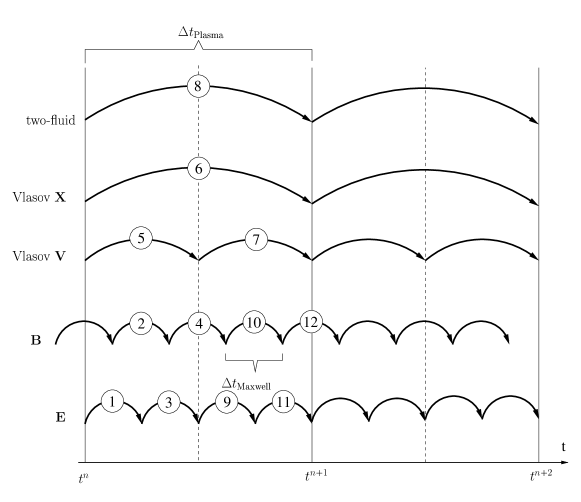
Figure 2: This is the order, in which the fields are updated in each step. Each arrow represents a substep of the respective scheme. The first line (two-fluid) represents the stepping of the fluid quantities. The update of the phase space density in physical (Vlasov X) and velocity space (Vlasov V) is separated by means of Strang splitting. The electric (E) and magnetic (B) field are updated separately.

As multistage and splitting methods are employed, care must be taken with respect to the points in time at which the fields and the fluxes at the cell faces live. Fig. 2 reveals the structure of time stepping for the electric E and magnetic B fields, the fluid quantities and the distribution functions. The timestep for the Maxwell solver is chosen to be smaller than the global timestep in order to resolve light waves which are much faster than all other speeds in the plasma. We choose the ratio between the smaller timestep of the Maxwell solver and the global timestep as a power of two, so the electromagnetic fields are known at all relevant times and the two different discrete times stay aligned throughout the simulation.

Initially, all the fields exist at the same point in time. Based on the currents calculated at that time, half a substep of the magnetic field is done in order to start the scheme. Afterwards, the following steps are repeated in a cyclic way:

1. Calculate currents from moments and phase space density of the different species and pass them to the Maxwell solver.

2. With these currents as source terms, advance the electromagnetic fields by half a global timestep. The magnetic field is shifted by half a time step, so linear interpolation is used for obtaining the magnetic field at the times at which the electric fields live.

3. Do a complete step of the Vlasov solver, which translates into half a step in velocity space, a full step in physical space and half a step in velocity space again. Herein, the new electromagnetic fields are used as source terms. The boundary conditions for the kinetic region are known from the last step.

4. Do a full step of the multi-fluid scheme. Once again, the newly obtained electromagnetic fields are used as source terms. The Runge-Kutta method requires boundary conditions at intermediate times, which must be obtained by temporal interpolation of the values provided by the Vlasov solver. Because of this, it is necessary to advance the plasma in the kinetic region first.

5. Now the currents can be calculated again.

6. With these, the electromagnetic field is advanced by another half step.

5 First Results of the multiphysics approach

As a first test, the GEM reconnection challenge setup, set forth in [1], was used. It was simulated both with the multifluid and the Vlasov code alone, as well as with our multiphysics coupling method.

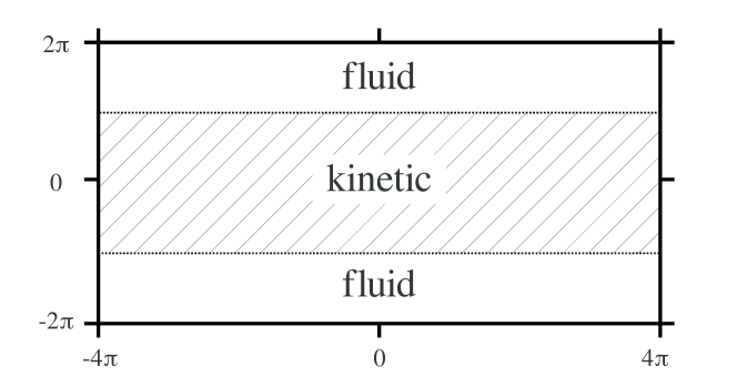
Figure 3: Partition of the domain of the GEM problem. The inner region (hatched), i.e. the vicinity of the current layer, is simulated by means of the kinetic model, whereas the multifluid code is employed in the outer regions.

For respecting the aforementioned restrictions, the vicinity of the current sheet was completely simulated by means of the Vlasov model and only in the outer regions the multifluid model was applied (see Fig. 3). Nevertheless, this already leads to nearly a half of the required computation time, as only half of the domain needs to be simulated with a kinetic code and the time needed for the multifluid code is negligible compared to that for the Vlasov code.
A comparison of the time needed for the respective simulations can be found in Tab. 1.

Code	System	Resolution	Time
multifluid	32 CPUs	$256\times 128$	0.3 h
Vlasov (cf. [22])	64 CPUs	$256\times 128\times 30\times 30\times 30$	150 h
Vlasov (this work)	64 CPUs / 64 GPUs	$256\times 128\times 32\times 32\times 32$	16 h
Vlasov/multifluid	64 CPUs / 64 GPUs	$256\times 128\,(\times\,32\times 32\times 32)$	8 h

Table 1: Comparison of the computational time required for solving the GEM reconnection challenge problem.

The results of the coupled simulation look both quantitatively and qualitatively the same as for the pure Vlasov simulation, which means that the region in which the determining physical processes occur is indeed the current layer and the multifluid model is sufficient for the outer region that was chosen (see Fig. 4 and Fig. 5).

As can be expected, a coupling inside the current sheet does not yield satisfactory results, because the simple 5-moment model leads to a different behaviour than the kinetic model. Thus, in future developments, new strategies will have to be developed in order to identify the regions which have to be treated by the kinetic or fluid description, respectively. This would result in an adaptive multiphysics approach to collisionless plasmas.

Figure 4: Comparison of reconnected flux vs. time for full kinetic (solid, taken from [22]), coupled (dashed), and pure multifluid (dotted) simulations.

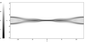
(a)

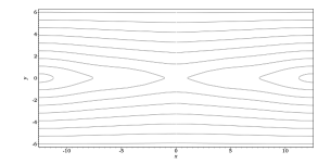
(b)

(c)

(d)

Figure 5: Comparison of $j_{z}$ and magnetic fieldlines between pure Vlasov and coupled simulation.

One problem, that is observed in general is the heating in the Vlasov region, due to numerical diffusivity in the velocity space, which can hardly be avoided. Especially the fast-gyrating electrons tend to be heated noticeably. This effect does not take place when the energy conservative multifluid code is used. This gives rise to a small yet observable temperature gradient at the coupling border and corresponding changes in other fields affected by it. As a quick fix, the numerical diffusivity can be lowered by a higher resolution in $v$-space. In the long run a more robust solution for this problem needs to be found.

6 Summary and Outlook

A Vlasov code on GPUs and a conventional multifluid code were presented that can be run both on their own as well as coupled to each other during runtime. Coupling of both codes was achieved by a combination of extrapolating and adjusting the distribution function according to the moments of the fluid description. Specific results on the GEM reconnection setup were extremely encouraging and a remarkable speed-up was observed . However, we should note that this is only a first step in the treatment of multiphysics descriptions of collisionless plasmas. Further steps needed to achieve this goal should include

1. appropriate closure relations (adiabatic, Chew-Goldberger-Low, isotropic, polytropic, Landau-fluid) depending on the physical situation;

2. an identification of regions which have to be treated by a kinetic or fluid description, respectively;

3. allowing the kinetic regions to change and move in an adaptive way in order to get the most efficient description of the underlying problem (analogous to our our adaptive mesh framework racoon [23]).

These topics are currently under development in our group.

References

- Birn et al. [2001] J. Birn, J. F. Drake, M. A. Shay, Geospace Environmental Modeling (GEM) Magnetic Reconnection Challenge, J. Geophys. Res. 106 (2001) 3715–3719.
- Woods [2006] L. Woods, Theory of Tokamak Transport, Wiley, 2006.
- Ramesh et al. [2005] R. Ramesh, A. Satya Narayanan, C. Kathiravan, C. V. Sastry, N. Udaya Shankar, An estimation of the plasma parameters in the solar corona using quasi-periodic metric type III radio burst emission, A & A 431 (2005) 353–357.
- Degond et al. [2010] P. Degond, G. Dimarce, L. Mieussens, A multiscale kinetic-fluid solver with dynamic localization of kinetic effects, J. Comput. Phys. 229 (2010) 4907–4933.
- Dellacherie [2003] S. Dellacherie, Kinetic-fluid coupling in the field of the atomic vapor isotopic separation: Numerical results in the case of a monospecies perfect gas, AIP Conf. Proc. 663 (2003) 947–956.
- Goudon et al. [2013] T. Goudon, S. Jin, J.-G. Liu, B. Yan, Asymptotic-preserving schemes for kinetic-fluid modeling of disperse two-phase flows., J. Comput. Phys. 246 (2013) 145–164.
- Klar et al. [2000] A. Klar, H. Neunzert, J. Struckmeier, Transition from kinetic theory to macroscopic fluid equations: A problem for domain decomposition and a source for new algorithms, Transport Theory and Statistical Physics 29 (2000) 93–106.
- Le Tallec and Mallinger [1997] P. Le Tallec, F. Mallinger, Coupling Boltzmann and Navier-Stokes Equations by Half Fluxes, Journal of Computational Physics 136 (1997) 51–67.
- Sugiyama and Kusano [2007] T. Sugiyama, K. Kusano, Multi-scale plasma simulation by the interlocking of magnetohydrodynamic model and particle-in-cell kinetic model, Journal of Computational Physics 227 (2007) 1340–1352.
- Markidis et al. [2014] S. Markidis, P. Henri, G. Lapenta, K. Rönnmark, M. Hamrin, Z. Meliani, E. Laure, The fluid-kinetic particle-in-cell method for plasma simulations, Journal of Computational Physics (2014).
- Kolobov and Arslanbekov [2012] V. Kolobov, R. Arslanbekov, Towards adaptive kinetic-fluid simulations of weakly ionized plasmas, Journal of Computational Physics 231 (2012) 839–869.
- Schulze et al. [2003] T. P. Schulze, P. Smereka, W. E, Coupling kinetic Monte-Carlo and continuum models with application to epitaxial growth, Journal of Computational Physics 189 (2003) 197 – 211.
- Schmitz and Grauer [2006a] H. Schmitz, R. Grauer, Comparison of time splitting and backsubstitution methods for integrating Vlasov’s equation with magnetic fields, Comp. Phys. Commun. 175 (2006a) 86–92.
- Schmitz and Grauer [2006b] H. Schmitz, R. Grauer, Darwin–Vlasov simulations of magnetised plasmas, J. Comput. Phys. 214 (2006b) 738–756.
- Leslie and Purser [1995] L. M. Leslie, R. J. Purser, Three-dimensional mass-conserving semi-Lagrangian scheme employing forward trajectories, Mon. Weather Rev. 123 (1995) 2551–2566.
- Filbet et al. [2001] F. Filbet, E. Sonnendrücker, P. Bertrand, Conservative numerical schemes for the Vlasov equation, J. Comput. Phys. 172 (2001) 166–187.
- Crouseilles et al. [2010] N. Crouseilles, M. Mehrenberger, E. Sonnendrücker, Conservative semi-Lagrangian schemes for Vlasov equations, J. Comput. Phys. 229 (2010) 1927–1953.
- Kurganov and Levy [2000] A. Kurganov, D. Levy, A Third-Order Semidiscrete Central Scheme for Conservation Laws and Convection-Diffusion Equations, SIAM J. Sci. Comput. 22 (2000) 1461–1488.
- Shu and Osher [1988] C. W. Shu, S. Osher, Efficient Implementation of Essentially Non-oscillatory Shock-Capturing Schemes, J. Comput. Phys. 77 (1988) 439–471.
- Yee [1966] K. S. Yee, Numerical Solution of Initial Boundary Value Problems Involving Maxwell’s Equations in Isotropic Media, IEEE Trans. Antennas Propag. 14 (1966) 302–307.
- Taflove and Brodwin [1975] A. Taflove, M. E. Brodwin, Numerical Solution of Steady-State Electromagnetic Scattering Problems Using the Time-Dependent Maxwell’s Equations, IEEE Trans. Microwave Theory Tech. 23 (1975) 623–630.
- Schmitz and Grauer [2006] H. Schmitz, R. Grauer, Kinetic Vlasov simulations of collisionless magnetic reconnection, Phys. Plasmas 13 (2006).
- Dreher and Grauer [2005] J. Dreher, R. Grauer, Racoon: A parallel mesh-adaptive framework for hyperbolic conservation laws, Parallel Computing 31 (2005) 913.