The limits of statistical significance of Hawkes processes fitted to financial data

Abstract

Many fits of Hawkes processes to financial data look rather good but most of them are not statistically significant. This raises the question of what part of market dynamics this model is able to account for exactly. We document the accuracy of such processes as one varies the time interval of calibration and compare the performance of various types of kernels made up of sums of exponentials. Because of their around-the-clock opening times, FX markets are ideally suited to our aim as they allow us to avoid the complications of the long daily overnight closures of equity markets. One can achieve statistical significance according to three simultaneous tests provided that one uses kernels with two exponentials for fitting an hour at a time, and two or three exponentials for full days, while longer periods could not be fitted within statistical satisfaction because of the non-stationarity of the endogenous process. Fitted timescales are relatively short and endogeneity factor is high but sub-critical at about 0.8.

I Introduction

Hawkes processes are a natural extension of Poisson processes in which self-excitation causes event clustering (Hawkes, 1971a, b). Originally applied to the modeling of earthquake occurrences (Ogata, 1988, 1999), they have proven to be useful in many fields (e.g. neuroscience, criminology and social networks modeling (Chornoboy et al., 1988; Pernice et al., 2012; Mohler et al., 2011; Crane and Sornette, 2008; Yang and Zha, 2013)). This is because of their tractability and the ever-increasing number of estimation methods (Marsan and Lengliné, 2008; Reynaud-Bouret and Schbath, 2010; Lewis and Mohler, 2011; Bacry et al., 2012a; Da Fonseca and Zaatour, 2013; Bacry and Muzy, 2014b). Since many types of financial market events such as mid-quote changes, extreme return occurrences or order submissions are clustered in time, Hawkes processes have become a standard tool in finance too.

In the context of market microstructure, Hawkes processes were first introduced by Bowsher (2007), who simultaneously analyzed trades time and mid-quotes changes with a multivariate framework. Two others pioneer approaches are the ones by Bauwens and Hautsch (2003) and Hewlett (2006) who focused on the durations between transactions. Subsequently, Large (2007) supplemented transaction data with limit orders and cancellations data in a ten-variate Hawkes process in order to measure the resilience of an London Stock Exchange order book. Bacry et al. (2012b) have recently modeled the mid-price change as the difference between two Hawkes processes and showed that the resulting price exhibits microstructure noise and the Epps effect. Jaisson and Rosenbaum (2013) established that under a suitable rescaling a nearly unstable Hawkes process converges to a Heston model. Bacry and Muzy (2014a) used an enhanced version of the model to account for market impact. Finally, Jedidi and Abergel (2013) modeled the full order book with a multivariate Hawkes setup and proved that the resulting price diffuses at large time scales. Remarkably, Hawkes processes are also applied to other financial topics such as VaR estimation (Chavez-Demoulin et al., 2005; Chavez-Demoulin and McGill, 2012), trade-through modeling (Toke and Pomponio, 2011), portfolio credit risk (Errais et al., 2010), or financial contagion across regions (Aït-Sahalia et al., 2010) and across assets (Bormetti et al., 2013).

It is widely accepted among researchers that only a small fraction of price movements is directly explained by external news releases (e.g. Cutler et al. (1989); Joulin et al. (2008)). Thus, the price dynamics is mostly driven by internal feedback mechanisms, which corresponds to what Soros calls “market reflexivity” (Soros, 1987). In the framework of Hawkes processes, endogeneity comes from self-excitation while the baseline activity rate is deemed exogenous (see Sec. II for a mathematical definition). In other words, these processes provide a straightforward way to measure the importance of endogeneity, for example in the E-mini S&P futures (Filimonov and Sornette, 2012; Hardiman et al., 2013). Filimonov and Sornette (2012) argued that the level of endogeneity has increased steadily in the last decade due to the advent of high-frequency and algorithmic trading. Hardiman et al. (2013) showed that it is only the short-term endogeneity (linked to increases of computer power and speed, and, indeed, HFT) that has increased over the years, while the endogeneity factor has been very stable and close to 1, the special value at which the process becomes totally self-referential and unstable. Fitting Hawkes processes to financial data requires some care: one should not use a single exponential self-excitation kernel (Hardiman et al., 2013), while many other biases may affect fits with long-tailed kernels on long time periods (Filimonov and Sornette, 2013).

Nobody claims that Hawkes process are the exact description of the whole dynamics of financial markets. However, testing the significance of the fits is not a current priority in the literature. Given the fact that the fits are usually visually satisfactory, it seems obvious that statistical significance may be obtained in some cases. Here, we wish to assess the extent (and the limits) of the explanatory power of Hawkes processes with several possibly types of parametric kernels, according to three statistical tests. One of the difficulties in obtaining significant fits come from jumps in trading activity such as those occurring when markets open and close. This is why we work on data from FX markets which have the advantage of operating continuously for longer periods. There may still be discontinuities, either implicit (e.g. fixing time) or explicit (e.g. week-end closures) in our FX data, but at least one day of FX data spans many more hours than one day of equity market data and is thus more suitable to our aim. Hence, a minori, one may extrapolate most of our failures to fit correct Hawkes processes to other types of data with more significant activity discontinuities.

The two other papers on FX data and Hawkes processes have a different focus than ours: Hewlett (2006) deals with the relatively illiquid EUR/PLN currency pair and uses a single-exponential kernel. Rambaldi et al. (2014) also use EBS data (with the same time resolution as ours) and studies the dynamics of best quotes around important news. Because our data set consists of order book snapshots every 0.1 s (see Sec. III for more details), we can trace most trades but not mid price changes. This is why we fit a univariate Hawkes process to EUR/USD trade arrivals. The endogeneity parameter is then the average number of trades triggered by a single trade.

The structure of the paper is as follows: we first define Hawkes processes, the fitting method, the parametric kernels and the statistical tests that we will use. We first show that Hawkes processes excel at fitting one hour of FX data, are fairly good for a single day, and fail when used for two consecutive days.

II Hawkes processes

An univariate Hawkes process is a linear self-exciting point process with an intensity given by

$$\lambda_{t} =\mu_{t}+\int_{0}^{t}\phi(t-s)dN_{s}$$

$$=\mu_{t}+\sum_{t_{i}<t}\phi(t-t_{i}),$$ (1)

where $\mu_{t}$ is a baseline intensity describing the arrival of exogenous events and the second term is a weighted sum over past events. The kernel $\phi(t-t_{i})$ describes the impact on the current intensity of a previous event that took place at time $t_{i}$.

A Hawkes process can be mapped to (and interpreted as) a branching process, where exogenous “mother” events occurring with intensity $\mu_{t}$ can trigger one or more “child” events. In turn, each of these children, can trigger multiple child events (or “grand-child” respectively to the original event), and so on. The quantity $n\equiv\int_{0}^{\infty}\phi(s)ds$ controls the size of the endogenously generated families. Indeed, $n$ is the branching ratio of the process, which is defined as the average number of children for any event. Therefore, $n$ quantifies market reflexivity in an elegant way. Three regimes exist depending on the branching ratio value:

• a sub-critical regime $(n<1)$ where families dies out almost surely,

• the critical regime $(n=1)$, where one family lives indefinitely without exploding. In the language of Hawkes process, this requires $\mu=0$ to be properly defined and it is equivalent to Hawkes process without ancestors studied by Brémaud and Massoulié (2001),

• the explosive regime $(n>1)$, where a single event triggers an infinite family with a strictly positive probability.

Evaluating $n$ gives a simple measure of the market “distance” to criticality. For $n\leq 1$, the process is stationary if $\mu_{t}$ is constant. In this case, the branching ratio is also equal to the average proportion of endogenously generated events among all events.

II.1 Parametric kernels

We compare the performance of the following kernels, each labeled by its own index.

• Sum of exponentials:

  $$\phi_{M}(t)=\sum_{i=1}^{M}\alpha_{i}e^{-t/\tau_{i}},$$

  where $M$ is the number of exponentials. The amplitudes $\alpha_{i}$ and timescales $\tau_{i}$ of the exponentials are the estimated parameters. The branching ratio is then given by: $n=\sum_{i=1}^{M}\alpha_{i}\tau_{i}=\sum_{i=1}^{M}n_{i}.$

• Approximations of power-laws have the advantage of needing a few parameters only. As a consequence, fitting them to data is much easier. Approximate power-law kernel is given by

  $$\phi_{M}^{{\scriptscriptstyle\text{PL}}}(t)=\frac{n}{Z}\sum_{i=0}^{M-1}a_{i}^{-(1+\epsilon)}e^{-\frac{t}{a_{i}}},$$

  where

  $$a_{i}=\tau_{0}m^{i}.$$

  $M$ controls the range of the approximation and $m$ its precision. $Z$ is defined such that $\intop_{0}^{\infty}\phi_{PL}(t)dt=n$. The parameters are the branching ratio $n$, the tail exponent $\epsilon$ and the smallest timescale $\tau_{0}$.

• Approximate power-law with a short lags cut-off (Hardiman et al., 2013):

  $$\phi_{M}^{{\scriptscriptstyle\text{HBB}}}(t)=\frac{n}{Z}\left(\sum_{i=0}^{M-1}a_{i}^{-(1+\epsilon)}e^{-\frac{t}{a_{i}}}-Se^{-\frac{t}{a_{-1}}}\right),$$

  the definition is the same as $\phi_{M}^{{\scriptscriptstyle\text{PL}}}$ with the addition of a smooth exponential drop for lags shorter than $\tau_{0}$. $S$ is defined such that $\phi_{M}^{{\scriptscriptstyle\text{HBB}}}(0)=0$.

• We propose a new type of kernels, made up of an approximate power-law $\phi_{M}^{{\scriptscriptstyle\text{PL}}}$ and one exponential with free parameters. This is to allow for a greater freedom in the structure of time scales. The kernel is then defined as

  $$\phi_{M}^{{\scriptscriptstyle\text{PL}_{\text{x}}}}(t)=\frac{n}{Z}\left(\sum_{i=0}^{M-1}a_{i}^{-(1+\epsilon)}e^{-\frac{t}{a_{i}}}+be^{-\frac{t}{\tau}}\right),$$

  where the exponential term adds two parameters $b$ and $\tau$. The other variables have the same meaning as above.

When a kernel is a sum of exponentials, one can exploit a recursive relation for the log-likelihood calculation that reduces the computational complexity from $\mathcal{O}(N^{2})$ to $\mathcal{O}(N)$ (see Ozaki (1979)). It provides reasonable computation time on a single workstation since N is $\mathcal{O}(10^{4})$. The first form is the most flexible and can approximate virtually any continuous function, at the cost of extra-parameters and more sloppiness (Waterfall et al., 2006). The second and third ones aim to reproduce the long memory observed in many market but are less flexible; their effective support may span well beyond the fitting period. The last one tries to combine the best of both worlds.

Once a kernel form is specified, we use the L-BFGS-B algorithm (Byrd et al., 1995) to estimate the parameters that maximize the log-likehood. For each fit we try different starting points to avoid local maxima.

Using multivariate Hawkes process to fit the arrival and the reciprocal influence of buy and sell trades systematically yields null cross-terms. Both buy and sell trades yield indistinguishable results; we therefore focus on buy trades.

II.2 Goodness-of-fits tests

The quality of the fits is assessed on the time-deformed series of durations $\left\{\theta_{i}\right\}$, defined by

$$\theta_{i}=\int_{t_{i-1}}^{t_{i}}\hat{\lambda}_{t}dt,$$

where $\hat{\lambda}$ is the estimated intensity and $\left\{t_{i}\right\}$ are the empirical timestamps. If a Hawkes process describes the data correctly, the $\theta_{i}$s must be (i) independent and (ii) exponentially distributed with unit rate. The maximum-likelihood estimation, by construction, tends to maximize the exponential nature of the $\theta$s, but not their independence. This explains why QQ-plots of the resulting $\theta$s are visually very satisfying as long as the kernel contains than more one exponential.

Visual checks of QQ-plots is only one of the available criteria, many of them being more precise and rigorous. Indeed, property (i) can be tested by the Ljung-Box test, which examines the null hypothesis of absence of auto-correlation in a given time-series. We use here a slight modification of the original test statistic from Ljung and Box (1978), defined as

$$Q=N(N+2)\sum_{k=2}^{h+1}\frac{\hat{\rho}_{k}^{2}}{n-k},$$

where $N$ is the sample size, $\hat{\rho}_{k}$ is the sample autocorrelation at lag $k,$ and $h$ is the number of lags being tested. Under the null, $Q$ follows a $\chi^{2}$ with $h$ degrees of freedom. Note that we start the sum at $k=2$ (instead of 1). This is because of the systematic small one-step anti-correlation introduced by the data cleaning procedure (Sec. III.2). In other words, we wish to test the absence of auto-correlation at lags that are unaffected by this procedure.

Property (ii) is assessed by two tests

1. Kolmogorov-Smirnov test (KS henceforth), based on the maximal discrepancy between the empirical cumulative distribution and the exponential cumulative distribution. The asymptotic distribution under the null is the Kolmogorov distribution. It is known to be a very (even excessively) demanding test.

2. Engle and Russell (1998) Excess Dispersion test (ED henceforth), which verifies the lack of excess dispersion in the residuals. The test statistic reads:

   $$S=\sqrt{N}\frac{\hat{\sigma}^{2}-1}{\sqrt{8}},$$

   where $\hat{\sigma}^{2}$ is the sample variance of $\theta$ which should be equal to $1.$ Under the null, $S$ has a limiting normal distribution.

All these three tests check basic but essential properties of the $\theta$s.

III data

III.1 Description

We study EUR/USD inter-dealer trading from January 1, 2012 to March 31, 2012. The data comes from EBS, the leading electronic trading platform for this currency pair. A message is recorded every 0.1 s. It contains the highest buying deal price and the lowest selling deal price with the dealt volumes, as well as the total signed volume of trades in the time-slice. Orders on EBS must have a volume multiple of 1 million of the base currency, which is therefore the natural volume unit. This is, to our knowledge, the best data available from EBS in terms of frequency (almost tick by tick) and, above all, has the invaluable advantage of containing information about traded volumes.

III.2 Treatment

The data must be filtered to improve the accuracy of fits. The coarse time resolution introduces a spurious discretization of the duration data, as illustrated in Fig. 1 (left plot). To overcome this issue, we added a time shift, uniformly distributed between $0$ and $0.1$, to trade occurrence times (Fig. 1, middle plot).

The number of transactions on one side during a time-slice can be determined from the total signed volumes in $92\%$ of cases. Indeed, when the total signed traded volume ($V_{total}$) is equal to the reported trade volume ($V_{report}$), only one trade occurred and the only uncertainty is about the exact time of the event. However, when $V_{total}>V_{report}$, one knows that more than one trade occurred. If $V_{total}-V_{report}=1$, exactly two trades occurred, one with volume $V_{report}$ and one with volume 1; their respective event time are randomly uniformly drawn during the time slice. Finally, the case $V_{total}-V_{report}>1$ (about $8\%$ of the non-empty time-slices) is ambiguous because the extra volume may come from more than one trade and hence may be split in different ways. We tried different schemes: not adding any trade, adding one trade, adding a trade per extra million, adding a uniform random number of trades between $1$ and $V_{total}-V_{report}$ and a self-consistent correction that uses the most probable partition according to the distribution of the volume of unambiguously determined trades. All of them give similar estimated fitting parameters for all kernels. However, statistical significance is best improved by adding one trade irrespective of the kernel choice . We therefore apply this procedure in this paper; as a consequence, all statistical results closely depend on this choice. The distribution of resulting durations are plotted in Fig 1 (right plot).

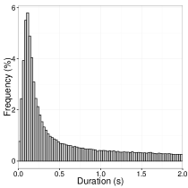
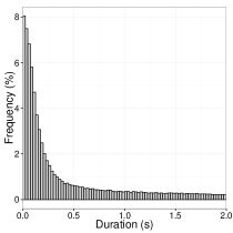
Figure 1: Duration distribution. Left: Raw times. Middle: Randomized times. Right: Corrected times. Three months of data, restricted to London active hours (9am-5pm).

This simple correction procedure introduces a weak, short-term memory effect. Figure 2 (left) plots the linear auto-correlation function of the sequence $\left\{\theta_{i}\right\}$, for a particular day (March 3rd 2012) (other days yield similar results). All the coefficients are almost statistically equal to zero except at the first lag (which is why we apply Ljung-Box test starting from the second lag). This negative value is induced by the correction procedure (see Sec. III.2) since the same measure performed in raw displays no memory at all (Fig. 2 (right)). The auto-correlation of the$\left\{(\theta_{i})^{2}\right\}$ series is however null with the correction procedure. This test therefore shows that the time stamp correction procedure, without which no fit ever passes a Kolmogorov-Smirnov test, is not entirely satisfactory from this point of view. Nevertheless, the side effects are small and most of the auto-correlation of the corrected timestamps is well explained by a Hawkes model.

There may be other unwanted side effects caused by limited time resolution and by the randomization of timestamps within a given interval. In particular, one may wonder if limited time resolution introduces a spurious small time scale in the fits. Appendix A reports extensive numerical simulations that assess the effect of limited time resolution and time stamp shuffling and shows first that this is not the case when time stamps are shuffled in an interval. In addition, the smallest fitted time scale is influenced by the limited time resolution, but to a limited extent.

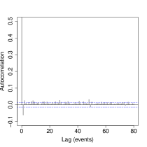
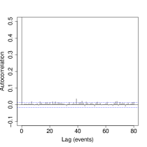
Figure 2: Time-adjusted durations autocorrelation function for March 3rd 2012. Left: with correction. Right: without correction.

IV Results

IV.1 Hourly fits

Hourly intervals are long enough to obtain reliable calibrations, at least on active hours during which 1500 events take place on average. In such short intervals, the endogenous activity $\mu_{t}$ in Eq. (1) can be approximated by a constant. We choose $m=2$ and $M=15$ for the power-law types of kernel. At the hourly scale, the results are fairly insensitive to changes in these parameters.

IV.1.1 Kernel comparisons

Table 1 summarizes the results of the 8 types of kernels for the three tests. The mono-exponential kernel $\phi_{1}$ is clearly much worse than all the other specifications and we can safely rule it out as a possible description of the data. Taking more than two exponentials only marginally improves the fits of hourly activity. QQ-plots (Fig. 3) illustrate the inadequacy of $\phi_{1}$ and show indeed that $\phi_{2}$ is a good kernel: for this time length, two time scales are enough to describe a whole hour of the arrival of FX trades. We judge the trade-off between log-likelihood and the number of parameters with Akaike criterion, denoted by $AIC_{p}$ , Akaike weights $w_{i}$ of kernel $i$, and $N_{max}$, the number of intervals in which kernel $i$ was the best. Both Akaike criteria are averaged over all the intervals. In the end, both $w_{i}$ and $N_{max}$ convey (almost) the same information because most of the time only one kernel has a weight almost equal to one. Power-law types of kernels also achieve good results, in particular $\phi_{15}^{{\scriptscriptstyle\text{PL}_{\text{x}}}}$, but all indicate a larger endogeneity factor $n$ than kernels with free exponentials. Akaike weights strongly suggest that $\phi_{2}$ is the best model at an hourly time scale. In addition we note that the means and medians of the fitted parameters of $\phi_{n}$ ($n=1,2,3$) kernels are very similar, while those of kernels that approximate power laws are significantly different, which points to the fact that this type of kernel is prone to fitting difficulties at an hourly time scale. Finally, the free exponential of $\phi_{15}^{{\scriptscriptstyle\text{PL}_{\text{x}}}}$ has a timescale of 0.06 s.

	$\phi_{1}$	$\phi_{2}$	$\phi_{3}$	$\phi_{15}^{{\scriptscriptstyle\text{HBB}}}$	$\phi_{15}^{{\scriptscriptstyle\text{PL}}}$	$\phi_{30}^{{\scriptscriptstyle\text{HBB}}}$	$\phi_{15}^{{\scriptscriptstyle\text{PL}}}$	$\phi_{15}^{{\scriptscriptstyle\text{PL}_{\text{x}}}}$
$\mu$	$0.13$	$0.08$	$0.08$	$0.07$	$0.07$	$0.07$	$0.07$	$0.06$
$n$	$0.41$	$0.64$	$0.64$	$0.67$	$0.67$	$0.77$	$0.75$	$0.72$
$\epsilon$	NA	NA	NA	$0.23$	$0.38$	$0.26$	$0.40$	$0.28$
$pKS$	$0.16$	$0.69$	$0.68$	$0.56$	$0.52$	$0.56$	$0.52$	$0.56$
$pED$	$0.03$	$0.57$	$0.55$	$0.63$	$0.60$	$0.58$	$0.57$	$0.62$
$pLB$	$0.11$	$0.38$	$0.38$	$0.34$	$0.31$	$0.29$	$0.28$	$0.33$
$\log\mathcal{L}_{p}$	$4022.9$	$4069.5$	$4069.9$	$4055.6$	$4062.9$	$4045.8$	$4060.3$	$4064.2$
$AIC_{p}$	$-8035.9$	$-8122.7$	$-8117.0$	$-8098.2$	$-8112.7$	$-8078.5$	$-8107.6$	$-8105.8$
$w$	$0.01$	$0.55$	$0.14$	$0.05$	$0.06$	$0.03$	$0.04$	$0.11$
$N_{max}$	$21$	$692$	$84$	$65$	$70$	$21$	$21$	$116$

Table 1: Comparison the ability of various kernels to fit Hawkes processes on hourly time windows. $pKS$, $pED$ and $pLB$ are respectively the Komogorov-Smirnov, Excess-Dispersion and Ljung-Box test average p-values. $\log\mathcal{L}_{p}$ is the log likelihood per point for the fit of each intervals, averaged over all intervals, and multiplied by the average number of points per interval. Idem for the Akaike information criterion $AIC_{p}$. The Akaike normalized weights $w[\phi]=\frac{1}{W}\exp\left(-\frac{AIC[\phi]-AIC_{min}}{2}\right)$, are the probabilites that kernel $\phi$ is the best according to Kullback–Leibler discrepancy (Wagenmakers and Farrell, 2004). $N_{max}[\phi]$ is the number of intervals in which the Akaike weight of kernel $\phi$ is the largest one. Values averaged over the fits on 1090 non-overlapping windows with more than 200 trades.

IV.1.2 Detailed results for $\phi_{2}$

Given its simplicity and good performance, it is interesting to look further into the results for the double exponential case. We note that Rambaldi et al. (2014) also suggest that this kernel is a good candidate for the modeling of mid-quotes changes in EBS data (without signed volumes). We characterize each hourly time-window by averaging the fits over three months.

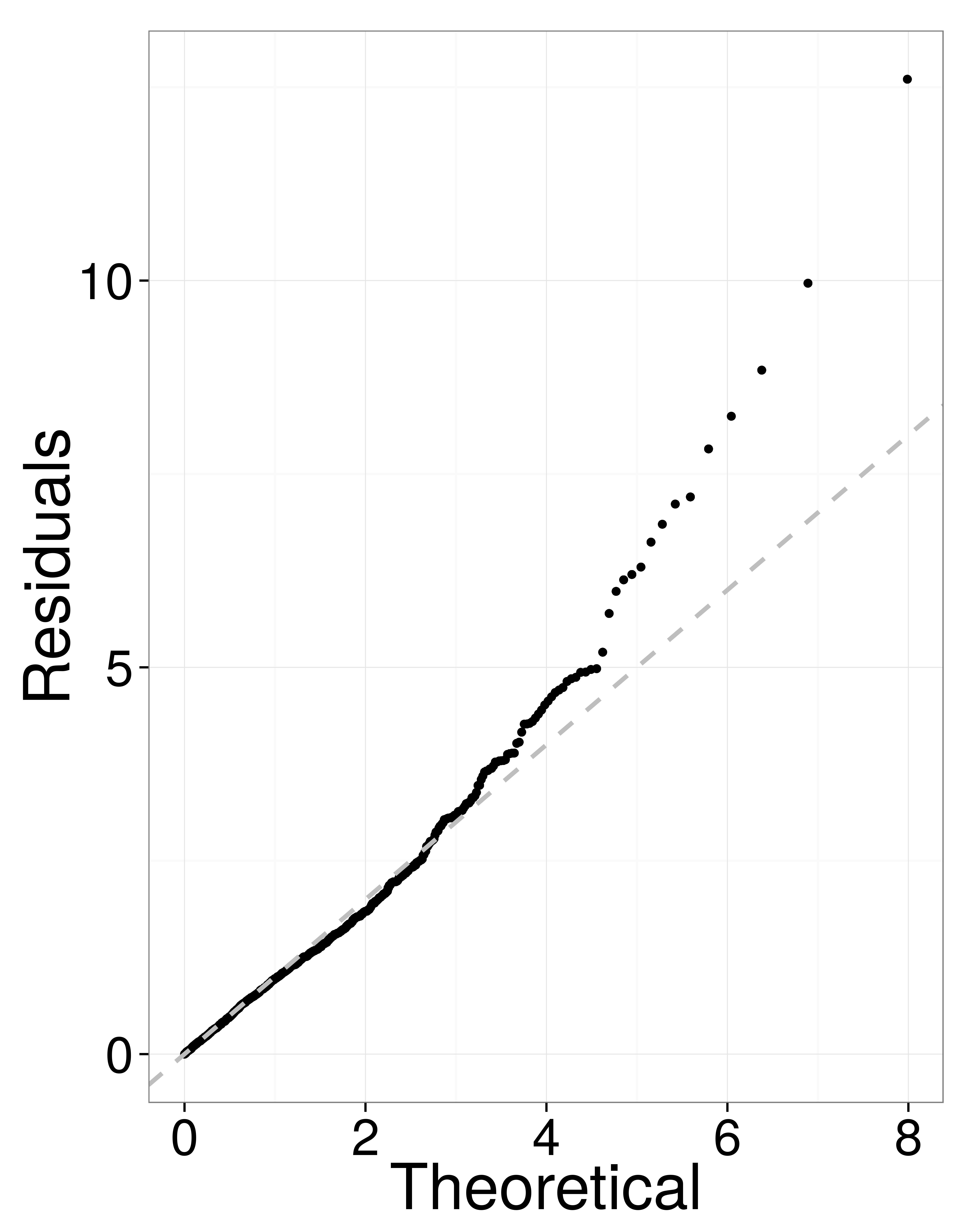
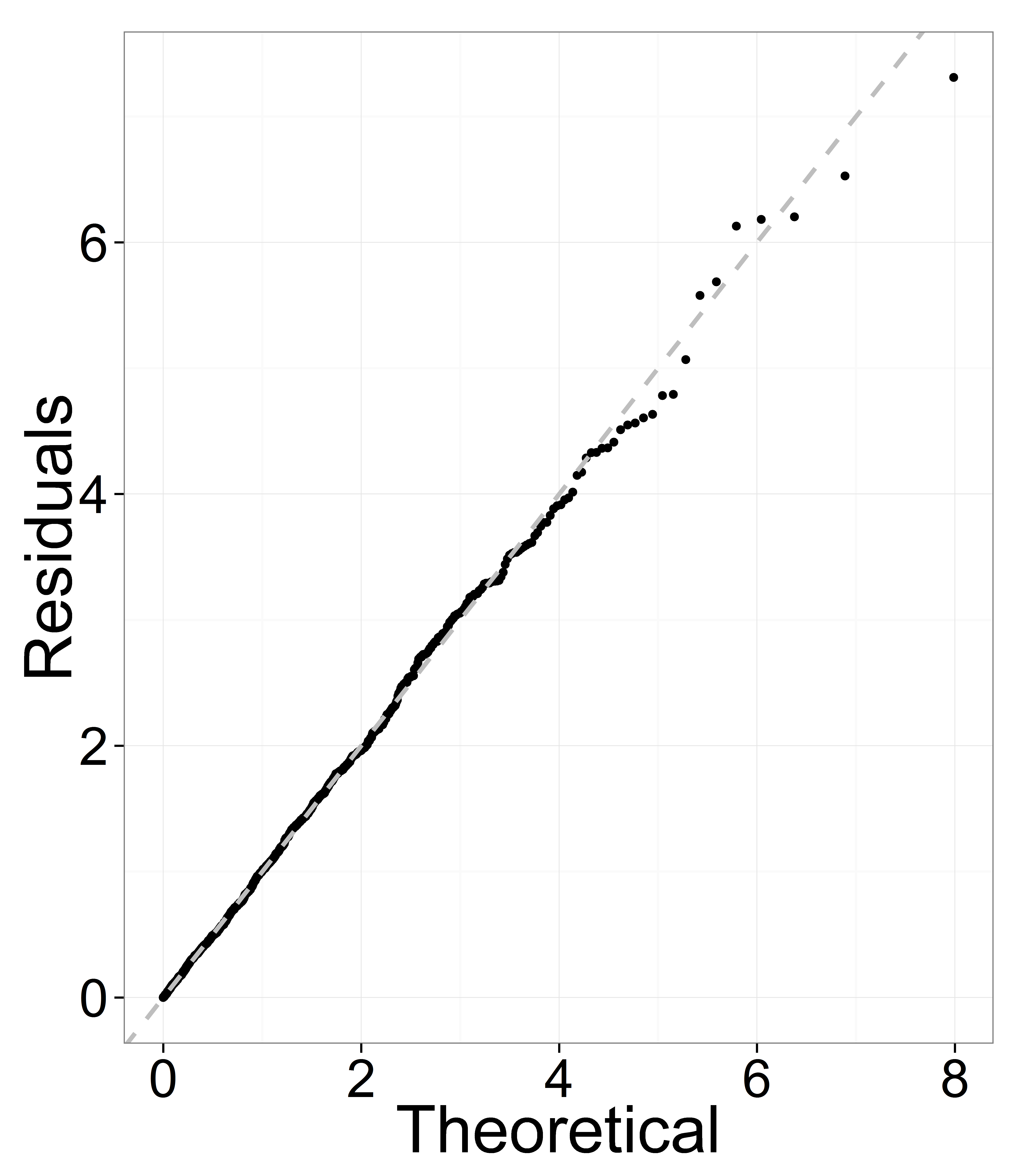
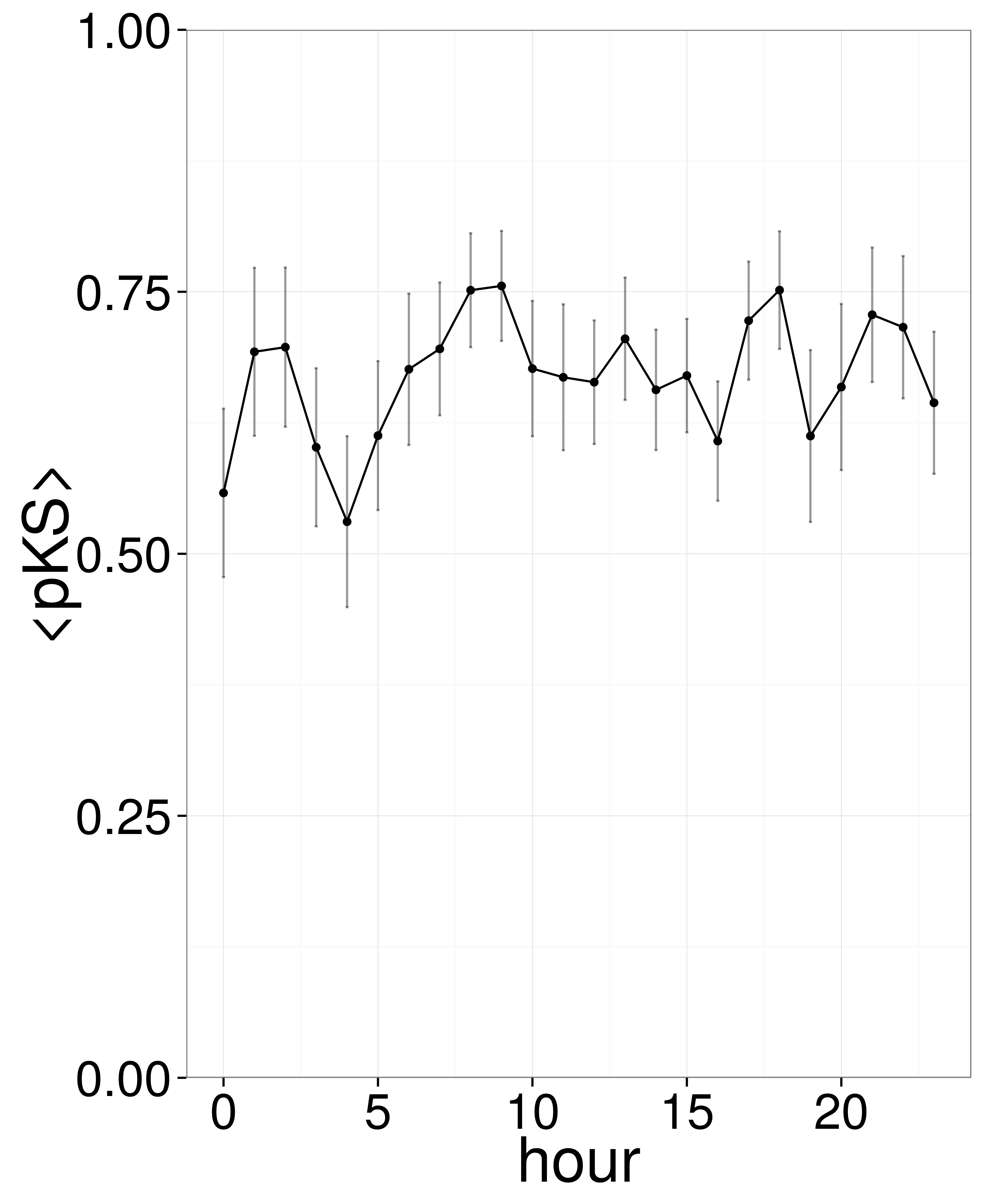
Figure 3: Goodness of Fit tests under the null hypothesis of exponentially distributed time-deformed durations. Left: A typical QQ-plot (February 1st 2012, 3-4pm) for $\phi_{1}$. Middle: Same for $\phi_{2}$. Right: Kolmogorov-Smirnov test average p-value. Error bars set at two standard deviations.

First, let us have a look at goodness of fits results. Fig. 3 (left plot) reports the quantiles of $\left\{\theta_{i}\right\}$ for a particular day and hourly window against the exponential theoretical quantiles. The fit is visually very satisfactory. Other time windows of all days yield similar results. Fig. 3 (right plot) demonstrates that all hours of the day pass Kolmogorov-Smirnov test by a large margin.

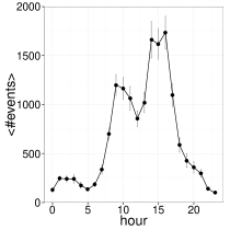
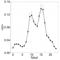
Figure 4: Left: Average number of trades (left) and average baseline intensity (right) throughout the day. Error bars set at two standard deviations.

In Fig. 4 (left), the number of trades displays the well-known intraday pattern of activity in the FX market (Dacorogna et al., 1993; Ito and Hashimoto, 2006). The average fitted exogenous part $\left\langle\mu\right\rangle$ perfectly reproduces this activity pattern (Fig. 4, right plot).

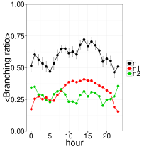
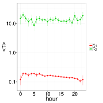
Figure 5: Average branching ratio throughout the day (left); black symbols: total ratio; green symbols: branching ratio of the largest time-scale; blue symbols: branching ratio of the smallest time-scale. Average associated times-scales on the right. Error bars set at two standard deviations.

Remarkably, the endogeneity level $n$ is relatively stable (within statistical uncertainty) for all hours (Fig. 5) given the fact that the typical trading activity is 10 times smaller at nights (Fig. 4). This is particularly striking for the endogeneity associated to largest time scale, $n_{2}$. Endogeneity associated with the smallest time scale, $n_{1}$, follows, albeit with a much smaller relative change, the daily average activity, except for the lunch time lull, which comes from the largest time scale. This suggests that while automated algorithmic trading takes no pause, human traders do have a break. In turn, this means that at this scale, most of the endogeneity at the smallest time scale comes from algorithmic trading, and that a sizable part of the endogeneity at longer times scales is caused by human trading.

IV.2 Whole-day fits

The relative stability of the branching ratio and the high p-values of e.g. KS tests encourages us to fit longer time windows. As we will see, this is possible for a full day at a time. In this case, $\mu$ cannot be considered constant anymore (see Fig. 4). As suggested by Bacry and Muzy (2014a), a time-of-the-day dependent background intensity is a good way to account for the intraday variation of activity. This method has the advantage of not mixing data from other days like classic detrending methods do. We thus approximate, for each day, $\mu_{t}$ by a piecewise linear function with knots at 0 am (when the series begin), 5 am, 9 am, 12 pm, 4 pm and at the end of the series. The $6$ knots values are additional fitting parameters.

IV.2.1 Kernel comparison

The results are synthesized in table 2.

Kernel	$\phi_{1}$	$\phi_{2}$	$\phi_{3}$	$\phi_{4}$	$\phi_{15}^{{\scriptscriptstyle\text{HBB}}}$	$\phi_{15}^{{\scriptscriptstyle\text{PL}}}$	$\phi_{15}^{{\scriptscriptstyle\text{HBB}}}/\mu_{cst}$	$\phi_{15}^{{\scriptscriptstyle\text{PL}}}/\mu_{cst}$	$\phi_{30}^{{\scriptscriptstyle\text{HBB}}}$	$\phi_{30}^{{\scriptscriptstyle\text{PL}}}$	$\phi_{15}^{{\scriptscriptstyle\text{PL}_{\text{x}}}}$
$n$	$0.48$	$0.79$	$0.83$	$0.85$	$0.81$	$0.83$	$0.92$	$0.93$	$0.98$	$0.97$	$0.88$
$pKS$	$7e-13$	$0.09$	$0.13$	$0.16$	$4\times 10^{-6}$	$2\times 10^{-7}$	$6\times 10^{-9}$	$6\times 10^{-10}$	$6\times 10^{-4}$	$4e-6$	$0.04$
$pED$	$0$	$0.10$	$0.31$	$0.45$	$0.61$	$0.51$	$0.6$	$0.54$	$0.52$	$0.49$	$0.66$
$pLB$	$0$	$0.058$	$0.056$	$0.012$	$9e-5$	$0.001$	$0.017$	$0.026$	$1\times 10^{-4}$	$2e-4$	$0.006$
$\log\mathcal{L}_{p}$	$60271.0$	$61559.3$	$61596.2$	$61575.5$	$61279.6$	$61340.2$	$61181.5$	$61271.1$	$61286.3$	$61340.6$	$61468$
$AIC_{p}$	$-120525.4$	$-123097.7$	$-123167.4$	$-123121.8$	$-122540.4$	$-122661.7$	$-122354.7$	$-122534.0$	$-122553.9$	$-122662.5$	$-122912.0$
$\epsilon$	NA	NA	NA	NA	$0.090$	$0.115$	$0.027$	$0.057$	$0.13$	$0.14$	$0.08$
$w$	$0$	$0.13$	$0.38$	$0.24$	$0$	$0$	$0$	$0$	$0$	$0$	$0.24$
$N_{max}$	$0$	$9$	$22$	$14$	$0$	$0$	$0$	$0$	$0$	$0$	$14$

Table 2: Kernel comparison. Full day fits. 59 points.

Only $\phi_{2}$ and $\phi_{3}$ pass the Ljung-Box test. This time $\phi_{3}$ is the favored model according to the Akaike weights and performs well with respect to the three tests. We note that $\phi_{15}^{{\scriptscriptstyle\text{PL}_{\text{x}}}}$, whose free exponential has a timescale equal to 0.11 s, is also a strong contender. We can gain a global insight across days from QQplots. Indeed, under the null hypothesis, the residuals possess the same distribution independently of the considered day. We therefore merge all the residuals from all the daily fits and construct the QQplot against the exponential distribution. Fig. 6 reports the performance of four families of kernel and bring a visual confirmation of the results in Table 2. In addition, it allows one to understand where each kernel performs best and worst. For example, $\phi_{30}^{{\scriptscriptstyle\text{PL}}}$ is better in the extreme tails than in the bulk of the distribution. One also sees the problems of $\phi_{3}$ in this region, solved by adding a fourth exponential (see $\phi_{4}$).

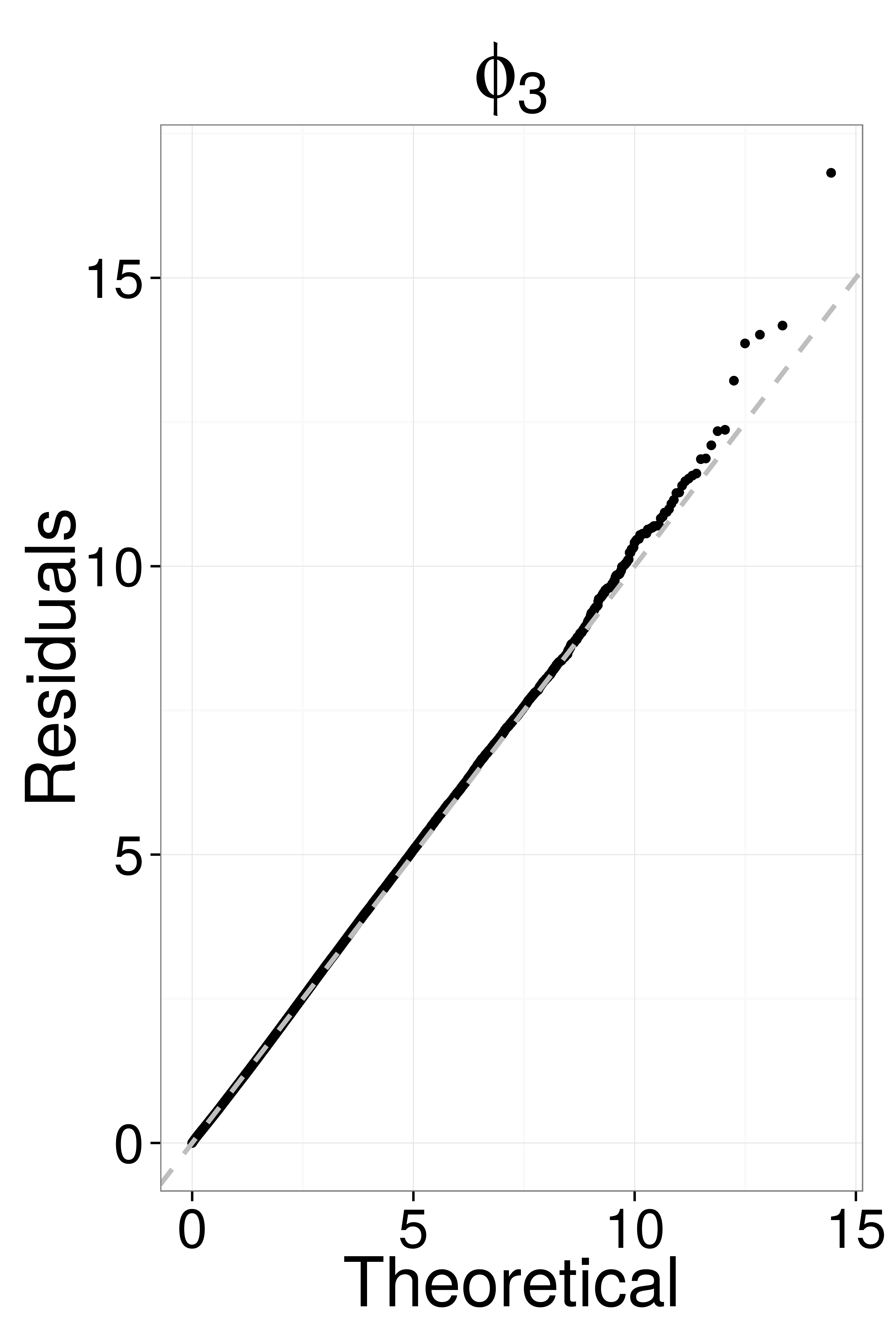
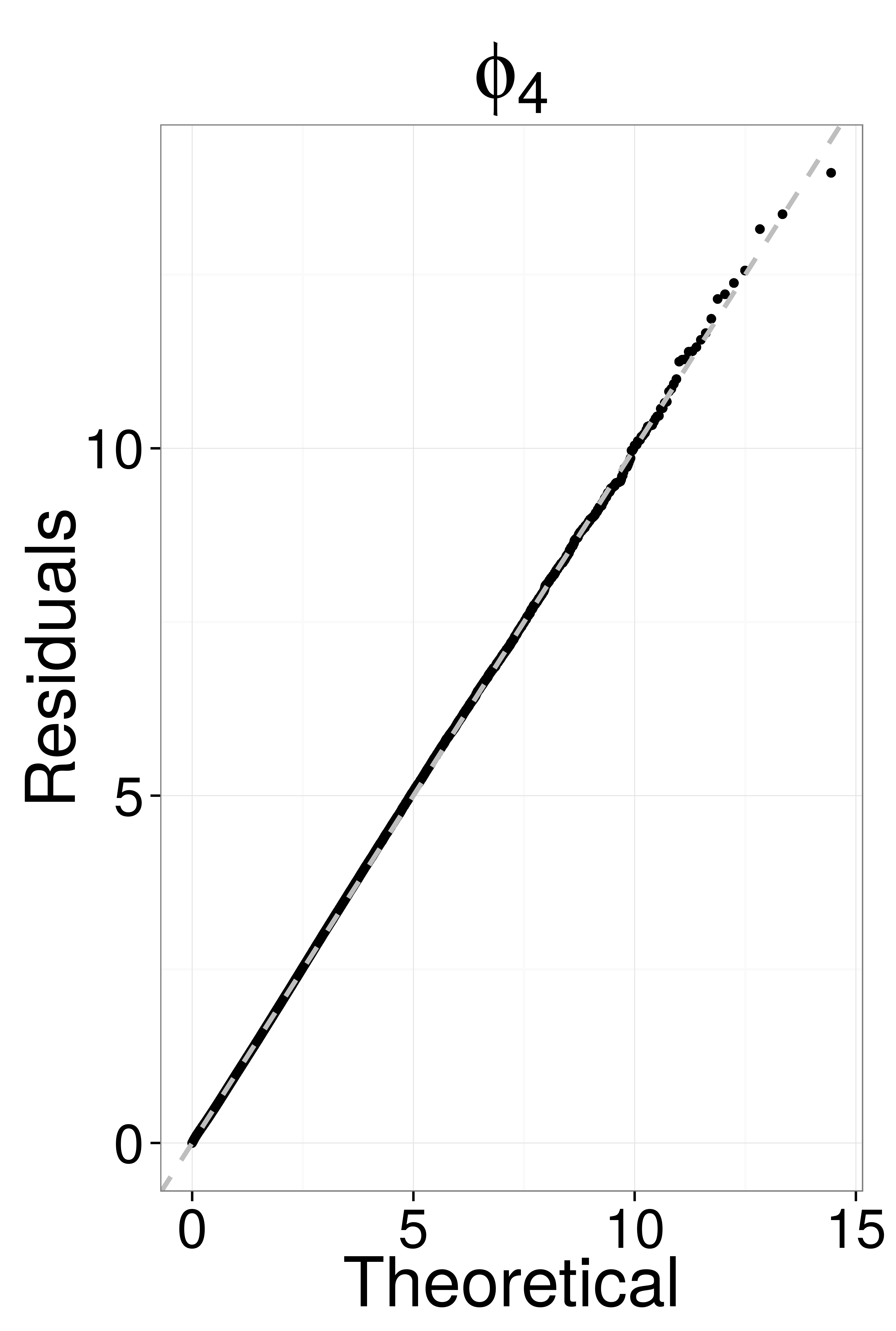
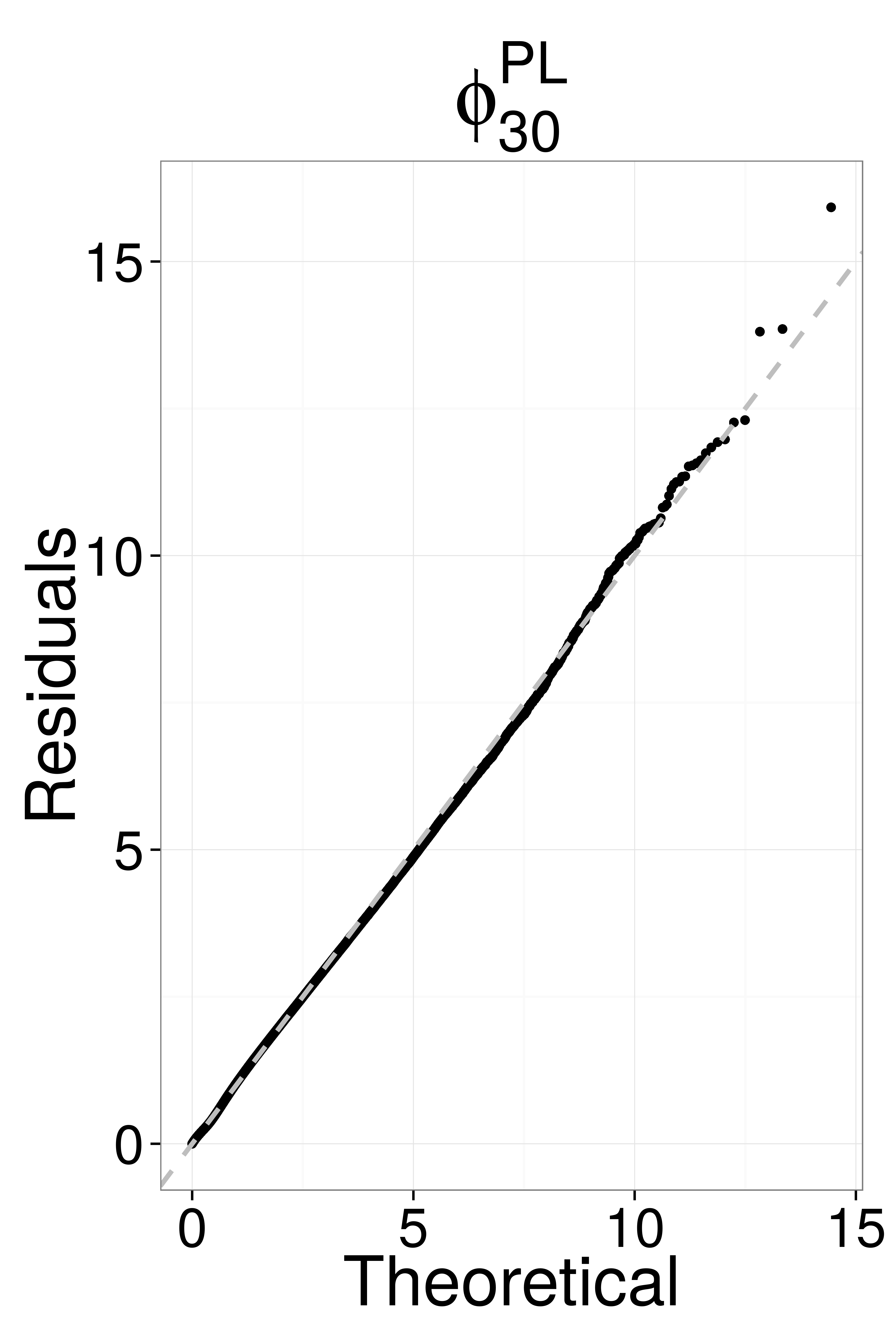
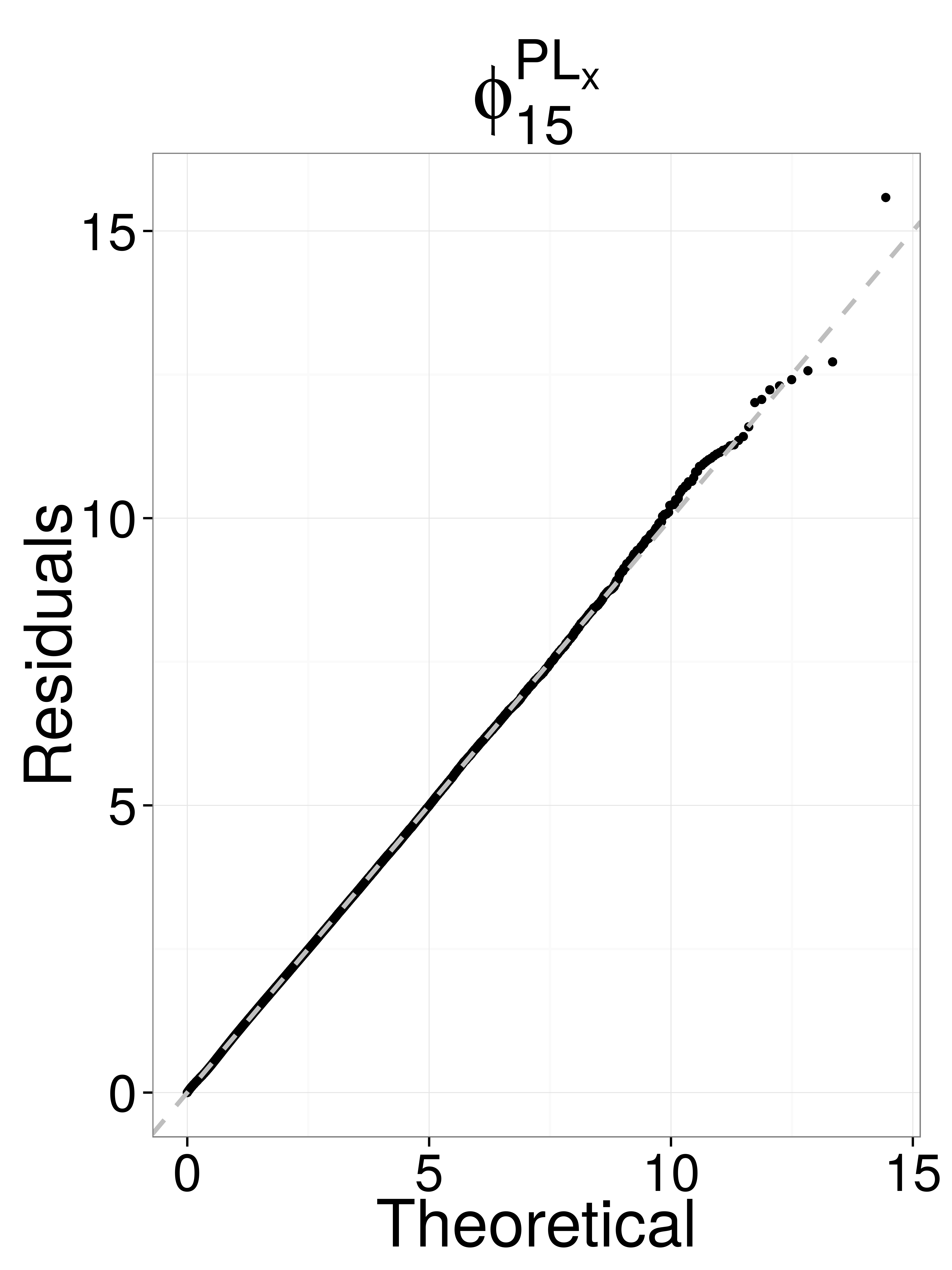
Figure 6: QQ-plot of the residuals merged from all intervals (one-day fits).

IV.2.2 Detailed results for $\phi_{3}$

Let us investigate in details the fits of $\phi_{3}$, the overall best kernel for whole days. We also show some results for $\phi_{2}$ for sake of comparison. The background intensity fitted values are summarized in Fig. 7 and are in line with the average intraday activity pattern.

Figure 7: Tukey boxplot of baseline intensity knots values.

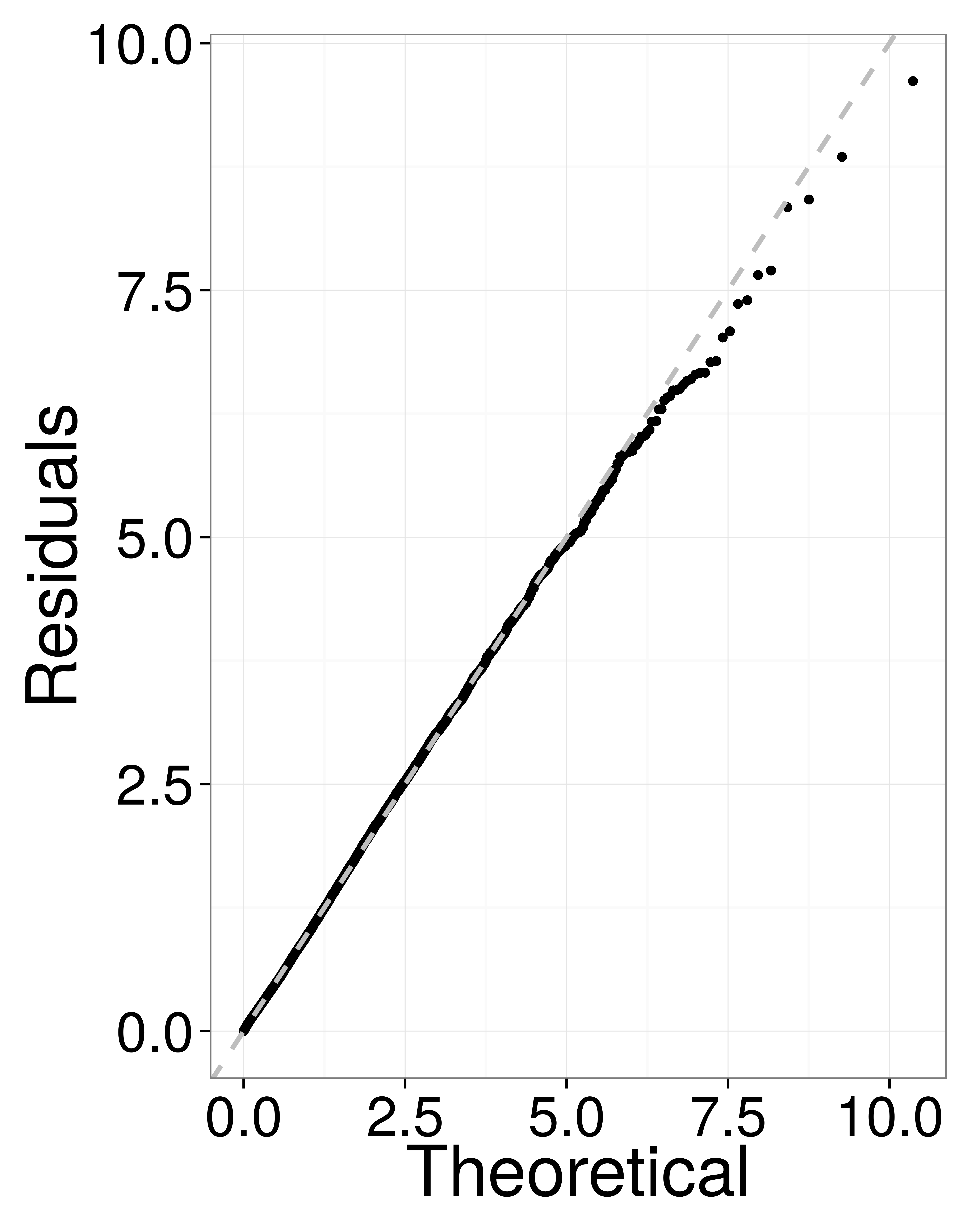
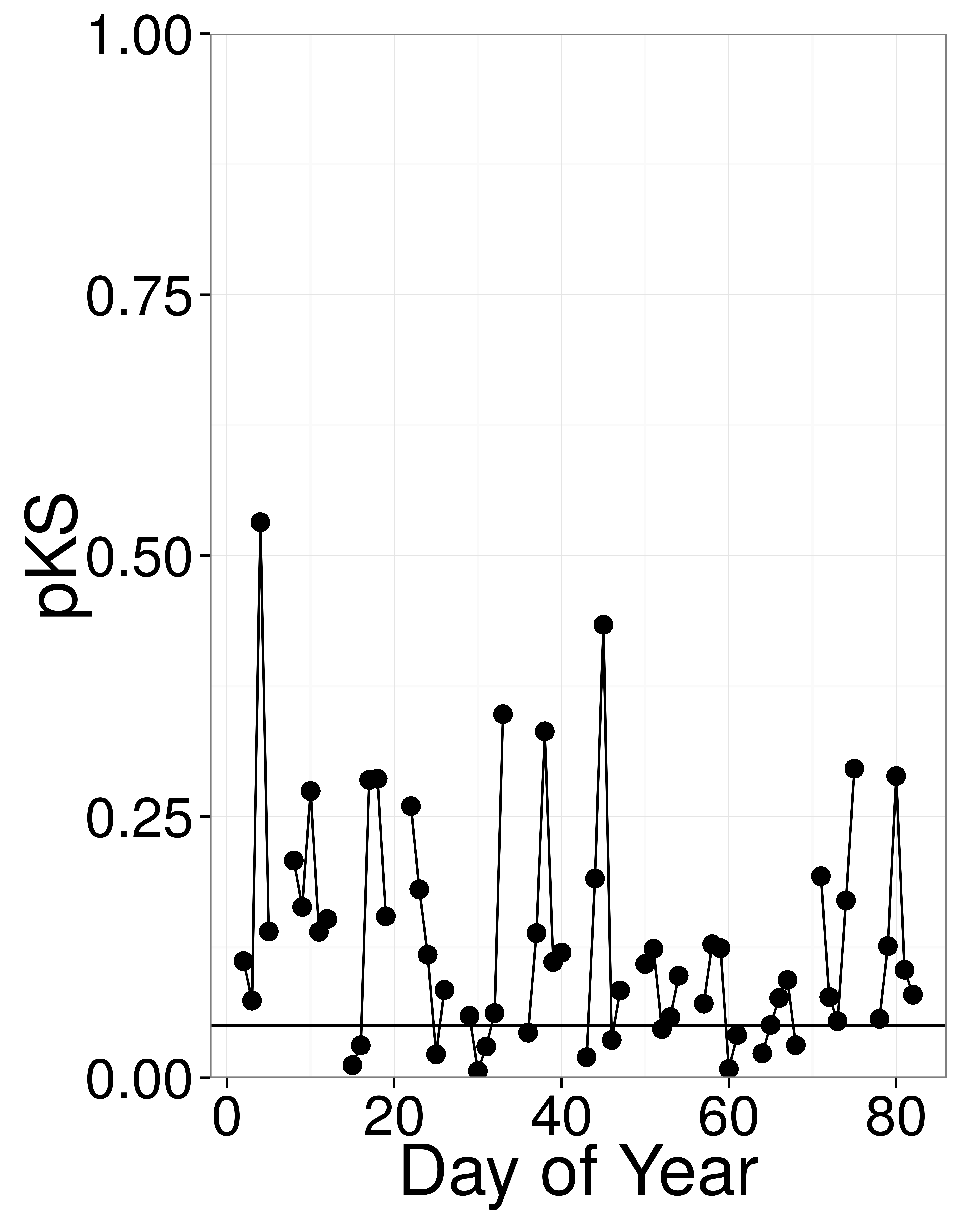
Figure 8: Goodness of Fit tests under the null hypothesis of exponentially distributed time-deformed durations. Left: A typical QQ-plot (March 3rd 2012). Right: Kolmogorov-Smirnov test p-value. The continuous line is the 0.05 significance level.

Figure 8 reports the Kolmogorov-Smirnov p-value for each fitted day. Again, the null hypothesis of exponentially distributed $\left\{\theta_{i}\right\}$, i.e., good fits, cannot be rejected. Fits are however less impressively significant that those of hourly fits case because of additional non-stationarities. On this plot and on all the remaining plots of the section, line breaks correspond to weekends. The QQ-plot (left plot of Fig. 8) visually confirms the accuracy of the fit.

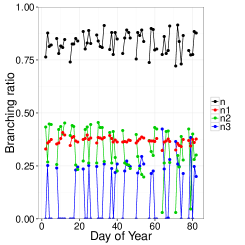
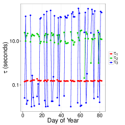
Figure 9: Daily branching ratio (left) and associated time-scales (right). The shortest characteristic timescale is very stable; the model captures $1$ or $2$ longer time scales depending on the day.

While the total branching ratio oscillates around 0.8 (Fig. 5), the parameters associated to each exponential make it clear that three timescales are only found on some days. This, once again, may either be because some days do not require three timescales, or because of the sloppiness of sums of exponentials. As reported by Table 3, the shortest timescale $\left\langle\tau_{1}\right\rangle$ does not depend on the effective number of timescales, while the second indeed does.

	2 timescales	3 timescales
$\left\langle\tau_{1}\right\rangle$	0.16 s	0.15 s
$\left\langle\tau_{2}\right\rangle$	21.9 s	9.3 s
$\left\langle\tau_{3}\right\rangle$	NA	161 s

Table 3: Average timescales when two or three timescales are found by fitting $\phi_{3}$ to whole days.

IV.3 Multi-day fits

Extending fits to two days requires to account for weekly seasonality. First and most importantly, EBS order book does not operate at week-ends, which implies that Mondays and Fridays most likely have a dynamics distinctly different from the other days. Thus we fit all pairs Tuesdays-Wednesdays, and Wednesdays-Thursdays, which amounts to 26 fits (2 points per week, 13 weeks). Before proceeding, it is important to keep in mind that Figure 7 forewarns that the daily variations of activity at various times of the day are ample, particularly at about 4pm, the time of the daily fixing. This may also prevent a single kernel to hold for several days in a row, the composition of the reaction times of the population of traders being potentially subject to similar fluctuations between two days.

Kernel	$\phi_{2}$	$\phi_{3}$	$\phi_{4}$	$\phi_{15}^{{\scriptscriptstyle\text{HBB}}}$	$\phi_{15}^{{\scriptscriptstyle\text{PL}}}$	$\phi_{30}^{{\scriptscriptstyle\text{HBB}}}$	$\phi_{30}^{{\scriptscriptstyle\text{PL}}}$	$\phi_{15}^{{\scriptscriptstyle\text{PL}_{\text{x}}}}$
$n$	$0.80$	$0.87$	$0.88$	$0.82$	$0.84$	$0.98$	$0.97$	$0.91$
$pKS$	$0.02$	$0.04$	$0.06$	$1\times 10^{-12}$	$3\times 10^{-15}$	$1\times 10^{-6}$	$3\times 10^{-10}$	$0.04$
$pED$	$0.04$	$0.46$	$0.54$	$0.50$	$0.35$	$0.59$	$0.44$	$0.58$
$pLB$	$0.010$	$0.008$	$0.011$	$2\times 10^{-6}$	$4\times 10^{-6}$	$3\times 10^{-8}$	$4\times 10^{-8}$	$0.001$
$\log\mathcal{L}_{p}$	$119666.0$	$119819.2$	$119814.5$	$119094.1$	$119221.6$	$119086.8$	$119207.4$	$119656.4$
$AIC_{p}$	$-239303.5$	$-239605.7$	$-239592.4$	$-238161.7$	$-238416.7$	$-238147.1$	$-238388.2$	$-239282.2$
$\epsilon$	NA	NA	NA	$0.08$	$0.11$	$0.13$	$0.15$	$0.10$
$w$	$0$	$0.34$	$0.40$	$0$	$0$	$0$	$0$	$0.26$
$N_{max}$	$0$	$9$	$10$	$0$	$0$	$0$	$0$	$7$

Table 4: Kernel comparison of two-days fits. 26 points.

Table 4 compares the performance of all kernels. Kernel $\phi_{2}$ performs poorly, while $\phi_{3}$, $\phi_{4}$ and $\phi_{15}^{{\scriptscriptstyle\text{PL}_{\text{x}}}}$ are the best ones according to $AIC_{p}$ criterion. No kernel can pass the three tests at the same time ($\phi_{3}$ does for a single pair of days). The timescales of $\phi_{3}$ are stable and similar to those of single-day fits ( $\left\langle\tau_{1}\right\rangle\simeq$ 0.15 s, $\left\langle\tau_{2}\right\rangle\simeq$ 10.6 s, $\left\langle\tau_{3}\right\rangle\simeq$ 178 s), while $\phi_{4}$ sometimes manages to find a fourth timescale. For the record, we tried to use 5 exponentials, but never found a fifth timescale. It is noteworthy that $\phi_{4}$ has an acceptable average pKS. The free exponential of $\phi_{15}^{{\scriptscriptstyle\text{PL}_{\text{x}}}}$ has a timescale of 0.13 s.

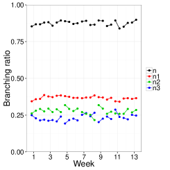
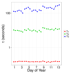
Figure 10: Endogeneity factors (left plot) and associated timescales (right plot) for fits of $\phi_{3}$ to two consecutive days

	3 timescales	4 timescales
$\left\langle\tau_{1}\right\rangle$	0.15 s	0.15 s
$\left\langle\tau_{2}\right\rangle$	13.5 s	7.1 s
$\left\langle\tau_{3}\right\rangle$	226 s	33 s
$\left\langle\tau_{4}\right\rangle$	NA	295 s

Table 5: Average timescales when three or four timescales are found by fitting $\phi_{4}$ to two consecutive days.

V Discussion and conclusions

Our results are mostly positive: Hawkes processes can indeed be fitted in a statistically significant way according to three tests to a whole day of data. This means that they describe very precisely a large number of events (around on average 15000). This is all the more remarkable because the fitted timescales are quite small. This shows that the endogenous part, which account for about 80% of the events, is limited to short time self-reactions in FX markets. This also means that at these time horizons, the instantaneous distribution of reaction time scales of the traders influences much the fitted kernels, as shown by the lunch lull in endogeneity. This is one reason why fitting more than one day with the same kernel is very hard since nothing guarantees that the composition of the trader population will be the same for several days in a row.

Fitting longer and longer time periods requires more and more exponentials. Fitting sums of exponentials with free parameters yields successive timescales whose ratios are not constant, which contrasts with the assumption of kernels that approximate power-laws. This is why the kernel $\phi_{15}^{{\scriptscriptstyle\text{PL}_{\text{x}}}}$, which adds one free exponential to the latter, has an overall better performance than pure approximations of power-laws. Longer time periods also leads to larger endogeneity factors, which makes sense since measuring long memory by definition requires long time series. As it clearly appears in all the tables, the use of power law-like kernels mechanically increases the apparent endogeneity factor, some of them being dangerously close to 1 (e.g $\phi_{30}^{{\scriptscriptstyle\text{HBB}}}$ and $\phi_{30}^{{\scriptscriptstyle\text{PL}}}$). That said, and quite importantly, the best kernels are never those with the largest endogeneity factors.

One may wonder if significance could be much improved by using data with a much better time resolution. It would certainly help, but only to a limited extent. As shown in Appendix A, only the KS test is affected by introduction of limited time resolution. Since the fits also fail to pass the the LB test for two consecutive days that is not affected by a limited time resolution, it is safe to assume that this failure has deeper reasons. The main problem resides in the difficulties caused by the non-stationarities of both exogeneity and endogeneity. The example of the lunch lull is striking: assuming a constant kernel shape for all times of the day, while a good approximation, cannot lead to statistical significance of fits over many days. In this precise case, one could add a daily seasonality on some weights.

Our results may well be specific to FX markets. In particular, the endogeneity is never close to 1, in contrast with studies on futures on equity indices. However given the nightly closure of equities markets (for example) and their short opening times, and given the difficulties encountered for FX data, it seems difficult to envisage a statistically satisfying comparison.

Appendix A Simulations

We simulate a Hawkes process with a $\phi_{2}$ kernel with parameters similar to those of hourly fits on real data: we set $\mu=0.05,$ $n_{1}=0.37$, $n_{2}=0.42$, $\tau_{2}=$21 s and vary $\tau_{1}$ from 0.05 s to 1.5 s. For each value of $\tau_{1}$ we perform $50$ simulations of $22$ hours. Then, on each simulated time-series, we artificially reduce the data resolution to 0.1 s, introducing time slicing as in our data set, and then randomize the timestamps within each time slice in order to mimic the procedure applied on empirical data (see Sec. III.2). We fit each resulting time-series and average the results over the $50$ runs with two- and three-exponential kernels.

Figure 11 reports the fitted smallest time scale as a function of the original time scale and shows that the shuffling of time stamps within an interval leads artifically increases the apparent smallest time scale, particularly (and quite expectedly) for small $\tau_{1}^{\mbox{sim}}$. Nevertheless, this increase is small, of the order of 15%. In addition, shuffling does not introduce a spurious third time scale, as fits with kernels with three exponentials did not yield any third time scale.

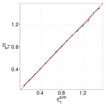
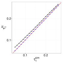
Figure 11: Fitted short timescale (black points) versus simulated short timescale. In red, the $y=x$ line. Right plot is a zoom on the critical region (close to 0.1 s). Blue points are the fitted values without the slicing procedure. Small distortion in the short timescale determination. Error bars set at two standard deviations..

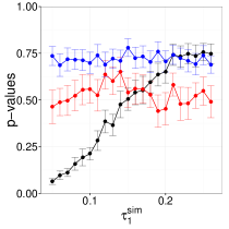
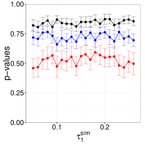
Figure 12: Fits p-values for Kolmogorov-Smirnov test (black), Ljung-Box test (red) and Excess-Dispersion test (blue). Left plot: with time stamp shuffling within a time slice. Right plot: without shuffling. Only the Kolmogorov-Smirnov p-value is affected by the data bundling. Error bars set at two standard deviations.

Finally, Fig. 12 shows that only the Kolmogorov-Smirnov p-values are affected by the time slicing and time stamp shuffling within a time slice. Nevertheless, at $\tau_{1}^{fit}=0.15\mbox{s}$ , $pKS$ is still larger than $0.05.$ This is consistent with fits on real data: significance is possible, but limited time resolution does not help.

References

- Aït-Sahalia et al. [2010] Yacine Aït-Sahalia, Julio Cacho-Diaz, and Roger J A Laeven. Modeling Financial Contagion Using Mutually Exciting Jump Processes. National Bureau of Economic Research Working Paper Series, No. 15850, 2010.
- Bacry et al. [2012a] E. Bacry, K. Dayri, and J. F. Muzy. Non-parametric kernel estimation for symmetric Hawkes processes. Application to high frequency financial data. The European Physical Journal B, 85(5):157, May 2012a.
- Bacry et al. [2012b] E Bacry, S Delattre, M Hoffmann, and J F Muzy. Modelling microstructure noise with mutually exciting point processes. Quantitative Finance, 13(1):65–77, January 2012b.
- Bacry and Muzy [2014a] Emmanuel Bacry and Jean-François Muzy. Hawkes model for price and trades high-frequency dynamics. Quantitative Finance, pages 1–20, April 2014a.
- Bacry and Muzy [2014b] Emmanuel Bacry and Jean-Francois Muzy. Second order statistics characterization of Hawkes processes and non-parametric estimation. January 2014b.
- Bauwens and Hautsch [2003] Luc Bauwens and Nikolaus Hautsch. Dynamic Latent Factor Models for Intensity Processes. CORE Discussion Paper, 103, February 2003.
- Bormetti et al. [2013] Giacomo Bormetti, Lucio Maria Calcagnile, Michele Treccani, Fulvio Corsi, Stefano Marmi, and Fabrizio Lillo. Modelling systemic price cojumps with Hawkes factor models. January 2013.
- Bowsher [2007] Clive G Bowsher. Modelling security market events in continuous time: Intensity based, multivariate point process models. Journal of Econometrics, 141(2):876–912, December 2007.
- Brémaud and Massoulié [2001] Pierre Brémaud and Laurent Massoulié. Hawkes Branching Point Processes without Ancestors. Journal of Applied Probability, 38(1):122–135, March 2001.
- Byrd et al. [1995] R Byrd, P Lu, J Nocedal, and C Zhu. A Limited Memory Algorithm for Bound Constrained Optimization. SIAM Journal on Scientific Computing, 16(5):1190–1208, September 1995.
- Chavez-Demoulin and McGill [2012] V Chavez-Demoulin and J A McGill. High-frequency financial data modeling using Hawkes processes. Journal of Banking & Finance, 36(12):3415–3426, December 2012.
- Chavez-Demoulin et al. [2005] V Chavez-Demoulin, A C Davison, and A J McNeil. Estimating value-at-risk: a point process approach. Quantitative Finance, 5(2):227–234, April 2005.
- Chornoboy et al. [1988] E S Chornoboy, L P Schramm, and A F Karr. Maximum likelihood identification of neural point process systems. Biological Cybernetics, 59(4-5):265–275, 1988.
- Crane and Sornette [2008] Riley Crane and Didier Sornette. Robust dynamic classes revealed by measuring the response function of a social system. Proceedings of the National Academy of Sciences, 105(41):15649–15653, October 2008.
- Cutler et al. [1989] David M Cutler, James M Poterba, and Lawrence H Summers. What moves stock prices? The Journal of Portfolio Management, 15(3):4–12, 1989.
- Da Fonseca and Zaatour [2013] José Da Fonseca and Riadh Zaatour. Hawkes process: Fast calibration, application to trade clustering, and diffusive limit. Journal of Futures Markets, pages n/a–n/a, 2013.
- Dacorogna et al. [1993] Michael M Dacorogna, Ulrich A Müller, Robert J Nagler, Richard B Olsen, and Olivier V Pictet. A geographical model for the daily and weekly seasonal volatility in the foreign exchange market. Journal of International Money and Finance, 12(4):413–438, August 1993.
- Engle and Russell [1998] Robert F Engle and Jeffrey R Russell. Autoregressive Conditional Duration: A New Model for Irregularly Spaced Transaction Data. Econometrica, 66(5):1127–1162, September 1998.
- Errais et al. [2010] E Errais, K Giesecke, and L Goldberg. Affine Point Processes and Portfolio Credit Risk. SIAM Journal on Financial Mathematics, 1(1):642–665, January 2010.
- Filimonov and Sornette [2012] Vladimir Filimonov and Didier Sornette. Quantifying reflexivity in financial markets: Toward a prediction of flash crashes. Physical Review E, 85(5):056108, May 2012.
- Filimonov and Sornette [2013] Vladimir Filimonov and Didier Sornette. Apparent criticality and calibration issues in the Hawkes self-excited point process model: application to high-frequency financial data. August 2013.
- Hardiman et al. [2013] Stephen J Hardiman, Nicolas Bercot, and Jean-Philippe Bouchaud. Critical reflexivity in financial markets: a Hawkes process analysis. Eur. Phys. J. B, 86(10), October 2013.
- Hawkes [1971a] Alan G Hawkes. Spectra of Some Self-Exciting and Mutually Exciting Point Processes. Biometrika, 58(1):83–90, April 1971a.
- Hawkes [1971b] Alan G Hawkes. Point Spectra of Some Mutually Exciting Point Processes. Journal of the Royal Statistical Society. Series B (Methodological), 33(3):438–443, January 1971b.
- Hewlett [2006] Patrick Hewlett. Clustering of order arrivals, price impact and trade path optimisation. In Workshop on Financial Modeling with Jump Processes, 2006.
- Ito and Hashimoto [2006] Takatoshi Ito and Yuko Hashimoto. Intraday seasonality in activities of the foreign exchange markets: Evidence from the electronic broking system. Journal of the Japanese and International Economies, 20(4):637–664, December 2006.
- Jaisson and Rosenbaum [2013] Thibault Jaisson and Mathieu Rosenbaum. Limit theorems for nearly unstable Hawkes processes. page 38, October 2013.
- Jedidi and Abergel [2013] Aymen Jedidi and Frederic Abergel. On the Stability and Price Scaling Limit of a Hawkes Process-Based Order Book Model. SSRN Electronic Journal, May 2013.
- Joulin et al. [2008] Armand Joulin, Augustin Lefevre, Daniel Grunberg, and Jean-Philippe Bouchaud. Stock price jumps: news and volume play a minor role. arXiv preprint arXiv:0803.1769, 2008.
- Large [2007] Jeremy Large. Measuring the resiliency of an electronic limit order book. Journal of Financial Markets, 10(1):1–25, February 2007.
- Lewis and Mohler [2011] E Lewis and G Mohler. A Nonparametric EM algorithm for Multiscale Hawkes Processes. Submitted, 2011.
- Ljung and Box [1978] G M Ljung and G E P Box. On a measure of lack of fit in time series models. Biometrika, 65(2):297–303, August 1978.
- Marsan and Lengliné [2008] David Marsan and Olivier Lengliné. Extending Earthquakes’ Reach Through Cascading. Science, 319(5866):1076–1079, February 2008.
- Mohler et al. [2011] G O Mohler, M B Short, P J Brantingham, F P Schoenberg, and G E Tita. Self-Exciting Point Process Modeling of Crime. Journal of the American Statistical Association, 106(493):100–108, March 2011.
- Ogata [1999] Y Ogata. Seismicity Analysis through Point-process Modeling: A Review. pure and applied geophysics, 155(2-4):471–507, 1999.
- Ogata [1988] Yosihiko Ogata. Statistical Models for Earthquake Occurrences and Residual Analysis for Point Processes. Journal of the American Statistical Association, 83(401):9–27, March 1988.
- Ozaki [1979] T Ozaki. Maximum likelihood estimation of Hawkes’ self-exciting point processes. Annals of the Institute of Statistical Mathematics, 31(1):145–155, 1979.
- Pernice et al. [2012] Volker Pernice, Benjamin Staude, Stefano Cardanobile, and Stefan Rotter. Recurrent interactions in spiking networks with arbitrary topology. Physical Review E, 85(3):31916, March 2012.
- Rambaldi et al. [2014] Marcello Rambaldi, Paris Pennesi, and Fabrizio Lillo. Modeling FX market activity around macroeconomic news: a Hawkes process approach. page 11, May 2014.
- Reynaud-Bouret and Schbath [2010] Patricia Reynaud-Bouret and Sophie Schbath. Adaptive estimation for Hawkes processes; application to genome analysis. pages 2781–2822, 2010.
- Soros [1987] Georges Soros. The Alchemy of Finance: Reding the Mind of the Market. 1987.
- Toke and Pomponio [2011] Ioane Muni Toke and Fabrizio Pomponio. Modelling Trades-Through in a Limited Order Book Using Hawkes Processes Trades-through. 2011.
- Wagenmakers and Farrell [2004] Eric-Jan Wagenmakers and Simon Farrell. AIC model selection using Akaike weights. Psychonomic Bulletin & Review, 11(1):192–196, 2004.
- Waterfall et al. [2006] Joshua J Waterfall, Fergal P Casey, Ryan N Gutenkunst, Kevin S Brown, Christopher R Myers, Piet W Brouwer, Veit Elser, and James P Sethna. Sloppy-Model Universality Class and the Vandermonde Matrix. Physical Review Letters, 97(15):150601, October 2006.
- Yang and Zha [2013] S. Yang and H. Zha. Mixture of Mutually Exciting Processes for Viral Diffusion. Journal of Machine Learning Research, 28(2):1–9, 2013.