A Credit Assignment Compiler for Joint Prediction

Abstract

Many machine learning applications involve jointly predicting multiple mutually dependent output variables. Learning to search is a family of methods where the complex decision problem is cast into a sequence of decisions via a search space. Although these methods have shown promise both in theory and in practice, implementing them has been burdensomely awkward. In this paper, we show the search space can be defined by an arbitrary imperative program, turning learning to search into a credit assignment compiler. Altogether with the algorithmic improvements for the compiler, we radically reduce the complexity of programming and the running time. We demonstrate the feasibility of our approach on multiple joint prediction tasks. In all cases, we obtain accuracies as high as alternative approaches, at drastically reduced execution and programming time.

1 Introduction

Many applications require a predictor to make coherent decisions. As an example, consider recognizing a handwritten word where each character might be recognized in turn to understand the word. Here, it is commonly observed that exposing information from related predictions (i.e. adjacent letters) aids individual predictions. Furthermore, optimizing a joint loss function can improve the gracefulness of error recovery. Despite these advantages, it is empirically common to build independent predictors, in settings where joint prediction naturally applies, because they are simpler to implement and faster to run. Can we make joint prediction algorithms as easy and fast to program and compute while maintaining their theoretical benefits?

Methods making a sequence of sub-decisions have been proposed for handling complex joint predictions in a variety of applications, including sequence tagging [30], dependency parsing (known as transition-based method) [35], machine translation [18], and co-reference resolution [44]. Recently, general search-based joint prediction approaches (e.g., [10, 12, 14, 22, 41]) have been investigated. The key issue of these search-based approaches is credit assignment: When something goes wrong do you blame the first, second, or third prediction? Existing methods often take two strategies:

• The system ignores the possibility that a previous prediction may have been wrong, different costs have different errors, or the difference between train-time and test-time prediction.

• The system may use handcrafted credit assignment heuristics to cope with errors that the underlying algorithm makes and the long-term outcomes of decisions.

Both approaches may lead to statistical inconsistency: when features are not rich enough for perfect prediction, the machine learning may converge sub-optimally.

In contrast, learning to search approaches [5, 11, 40] automatically handle the credit assignment problem by decomposing the production of the joint output in terms of an explicit search space (states, actions, etc.); and learning a control policy that takes actions in this search space. These have formal correctness guarantees which differ qualitatively from graphical models such as the Conditional Random Fields [28] and structured SVMs [46, 47]. Despite the good properties, none of these methods have been widely adopted because the specification of a search space as a finite state machine is awkward and naive implementations do not fully demonstrate the ability of these methods.

Algorithm 1 MyRun(X) % for sequence tagging, X: input sequence, Y: output

1:  Y $\leftarrow$ []

2:  for t = 1 to len(X) do

3:     ref $\leftarrow$ X[t].true_label

4:     Y[t] $\leftarrow$ predict(x=examples[t], y=ref, tag=t, condition=[1:t-1])

5:  loss(number of Y[t] $\neq$ X[t].true_label)

6:  return Y

In this paper, we cast learning to search into a credit assignment compiler with a new programming abstraction for representing a search space. Together with several algorithmic improvements, this radically reduces both the complexity of programming and the running time. The programming interface has the following advantages:

• The same decoding function (see Alg. 1 and Sec. 2 for example) is used for training and prediction so a developer need only code desired test time behavior and gets training “for free. ” This simple implementation prevents common train/test asynchrony bugs.

• The compiler automatically ensures the model learns to avoid compounding errors and makes a sequence of coherent decisions.

• The library functions are in a reduction stack so as base classifiers and learning to search approaches improve, so does joint prediction performance.

Without extra implementation cost, implementations enabled by the credit assignment compiler achieve outstanding empirical performance both in accuracy and in speed. This provides strong simple baselines for future research and demonstrates the compiler approach to solving complex prediction problems may be of broad interest.

2 Programmable Learning to Search

We first describe the proposed programmable joint prediction paradigm. Algorithm 1 shows sample code for a part of speech tagger (or generic sequence labeler) under Hamming loss. The algorithm takes as input a sequence of examples (e.g., words), and predicts the meaning of each element in turn. The $i$th prediction depends on previous predictions. It uses two underlying library functions, predict(…) and loss(…). The function predict(…) returns individual predictions based on $x$ while loss(…) allows the declaration of an arbitrary loss for the point set of predictions. The loss(…) function and the reference $y$ inputted to predict(…) are only used in the training phase and it has no effect in the test phase. Surprisingly, this single library interface is sufficient for both testing and training, when augmented to include label “advice” from a training set as a reference decision (by the parameter $y$). This means that a developer only has to specify the desired test time behavior and gets training with minor additional decoration. The underlying system works as a credit assignment compiler to translate the user-specified decoding function and labeled data into updates of the learning model.

How can you learn a good predict function given just an imperative program like Algorithm 1? In the following, we show that it is essential to run the MyRun(…) function (e.g., Algorithm 1) many times, “trying out” different versions of predict(…) to learn one that yields low loss(…). We begin with formal definitions of joint prediction and a search space.

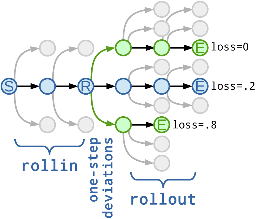
The system begins at the start state $S$ and chooses the middle action twice according to the rollin policy. At state $R$ it considers both the chosen action (middle) and one-step deviations from that action (top and bottom). Each of these deviations is completed using the rollout policy until reaching an end state, at which point the loss is collected. Here, we learn that deviating to the top action (instead of middle) at state $R$ decreases the loss by $0.2$.

Figure 1: A search space implicitly defined by an imperative program.

Joint Prediction.

Joint prediction aims to induce a function $f$ such that for any $X\in\mathcal{X}$ (the input space), $f$ produces an output $f(X)=Y\in\mathcal{Y}(X)$ in a (possibly input-dependent) space $\mathcal{Y}(X)$. The output $Y$ often can be decomposed into smaller pieces (e.g., $y_{1},y_{2},\ldots$), which are tied together by features, by a loss function and/or by statistical dependence. There is a task-specific loss function $\ell:\mathcal{Y}\times\mathcal{Y}\rightarrow\mathbb{R}^{\geq 0}$, where $\ell(Y^{*},\hat{Y})$ tells us how bad it is to predict $\hat{Y}$ when the true is $Y^{*}$.

Search Space.

In our framework, the joint variable $\hat{Y}$ is produced incrementally by traversing a search space, which is defined by states $s\in S$ and a mapping $A:S\rightarrow 2^{S}$ defining the set of valid next states. One of the states is a unique start state $S$ while some of the others are end states $e\in E$. Each end state corresponds to some output variable $Y_{e}$. The goal of learning is finding a function $f:X_{s}\rightarrow S$ that uses the features of an input state ($x_{s}$) to choose the next state so as to minimize the loss $\ell(Y^{*},Y_{e})$ on a holdout test set. Follow reinforcement learning terminology, we call the function a policy and call the learned function $f$ a learned policy $\pi_{f}$.

Turning Search Space into an Imperative Program

The definition of a TDOLR program: • Always terminate. • Takes as input any relevant feature information $X$. • Make zero or more calls to an oracle $O:X^{\prime}\rightarrow Y$ which provides a discrete outcome. • Report a loss $L$ on termination.

Algorithm 2 TDOLR(X) 1:  s $\leftarrow$ a 2:  while s $\not\in$ E do 3:     Compute $x_{s}$ from X and s 4:     s $\leftarrow$ O($x_{s}$) 5:  return  Loss(s)

Figure 2: Left: the definition; right: A TDOLR program simulates the search space.

Surprisingly, search space can be represented by a class of imperative program, called Terminal Discrete Oracle Loss Reporting (TDOLR) programs. The formal definition of TDOLR is listed in Figure 2. Without loss of generality, we assume the number of choices is fixed in a search space, and the following theorem holds:

Theorem 1.

For every TDOLR program, there exist an equivalent search space and for every search space there exists an equivalent TDOLR program.

Proof.

A search space is defined by $(A,E,S,l)$. We show there is a TDOLR program which can simulate the search space in algorithm 2. This algorithm does a straightforward execution of the search space, followed by reporting of the loss on termination. This completes the second claim.

For the first claim, we need to define, $(A,E,S,l)$ given a TDOLR program such that the search space can simulate the TDOLR program. At any point in the execution of TDOLR, we define an equivalent state $s=(O(X_{1}),...,O(X_{n}))$ where $n$ is the number of calls to the oracle. We define $a$ as the sequence of zero length, and we define $E$ as the set of states after which TDOLR terminates. For each $s\in E$ we define $l(s)$ as the loss reported on termination. This search space manifestly outputs the same loss as the TDOLR program. ∎

The practical implication of this theorem is that instead of specifying search spaces, we can specify a TDOLR program (such as Algorithm 1), radically reducing the programming complexity of joint prediction.

3 Credit Assignment Compiler for Training Joint Predictor

Now, we show how credit assignment compiler turn a TDOLR program and training data into model updates. In the training phase, the supervised signals are used in two places: 1) to define the loss function, and 2) to construct a reference policy $\pi^{*}$. The reference policy returns at any prediction point a “suggestion” as to a good next state. The general strategy is, for some number of epochs, and for each example $(X,Y)$ in the training data, to do the following:

1. Execute MyRun(…) on $X$ with a rollin policy to obtain a trajectory of actions $\vec{a}$ and loss $\ell_{0}$

2. Many times:

   1. For some (or for all) time step $t\leq|\vec{a}|$

   2. For some (or for all) alternative action $a_{t}^{\prime}\neq a_{t}$ ($a_{t}$ is the action taken by $\vec{a}$ in time step $t$)

   3. Execute MyRun(…)  on $X$, with predict returning $a_{1:t-1}$ initially, then $a_{t}^{\prime}$, then acting according to a rollout policy to obtain a new loss $\ell_{t,a_{t}^{\prime}}$

   4. Compare the overall losses $\ell_{t,a_{t}}$ and $\ell_{t,a_{t}^{\prime}}$ to construct a classification/regression example that demonstrates how much better or worse $a_{t}^{\prime}$ is than $a_{t}$ in this context.

3. Update the learned policy

The rollin and rollout policies can be the reference $\pi^{*}$, the current classifier $\pi_{f}$ or a mixture between them. By varying them and the manner in which classification/regression examples are created, this general framework can mimic algorithms like Searn [11], DAgger [41], AggreVaTe [40], and LOLS [5].

Algorithm 3 Learn(X, f)

1:  T, ex, cache $\leftarrow$ 0, [], []

2:  define Predict(x, y) := { T++ ; ex[T-1] $\leftarrow$ x; cache[T-1] $\leftarrow$ f(x, y, rollin) ; return  cache[T-1]  }

3:  define Loss(l) := no-op

4:  MyRun(X)

5:  for $t_{0}$ $={\color[rgb]{0.2,0.2,0.2}\textit{1}}$ to T do

6:     losses, t $\leftarrow$ $\langle$0, 0, …, 0$\rangle$, 0

7:     for $a_{0}$ $={\color[rgb]{0.2,0.2,0.2}\textit{1}}$ to A(ex[$t_{0}$]) do

8:        Define Predict(x, y) := { t++ ; return  $\left\{\begin{array}[]{ll}\textnormal{{\color[rgb]{0.0,0.0,0.5}{cache}}$[${\color[rgb]{0.0,0.0,0.5}{t}}-1$]$}&\textnormal{if }t<t_{0}\\ \textnormal{{\color[rgb]{0.0,0.0,0.5}{$a_{0}$}}}&\textnormal{if }t=t_{0}\\ \textnormal{{\color[rgb]{0.4,0.0,0.4}{f}}({\color[rgb]{0.0,0.0,0.5}{x}},{\color[rgb]{0.0,0.0,0.5}{y}},{rollout})}&\textnormal{if }t>t_{0}\end{array}\right.$ }

9:        Define Loss(val) := { losses[$a_{0}$] += val }

10:        MyRun(X)

11:     Online update with cost-sensitive example (ex[$t_{0}$], losses)

The full learning algorithm (for a single joint input X) is depicted in Algorithm 3. In lines 1–4, a rollin pass of MyRun is executed. MyRun can generally be any TDOLR program as discussed (e.g., Alg. 1). In this pass, predictions are made according to the current policy, f, flagged as rollin (this is to enable support of arbitrary rollin and rollout policies). Furthermore, the examples (feature vectors) encountered during prediction are stored in ex, indexed by their position in the sequence (T), and the rollin predictions are cached in the variable cache (see Sec. 4).

The algorithm then initiates one-step deviations from this rollin trajectory. For every time step, (line 5), we generate a single cost-sensitive classification example; its features are ex[$t_{0}$], and there are m(ex[$t_{0}$]) possible labels (=actions). For each action (line 7), we compute the cost of that action by executing MyRun again (line 10) with a “tweaked” Predict which returns the cached predictions at steps before $t_{0}$, returns the perturbed action $a_{0}$ at $t_{0}$, and at future timesteps calls f for rollouts. The Loss function accumulates the loss for the query action. Finally, a cost-sensitive classification example is generated (line 11) and fed into an online learning algorithm.

4 Optimizing the Credit Assignment Compiler

We present two algorithmic improvements which make training orders of magnitude faster.

Optimization 1: Memoization

The primary computational cost of Alg. 3 is making predictions: namely, calling the underlying classifier in Step 10. In order to avoid redundant predictions, we cache previous predictions. The challenge is understanding how to know when two predictions are going to be identical, faster than actually computing the prediction. To accomplish this, the user may decorate calls to the Predict function with tags. For a graphical models, a tag is effectively the “name” of a particular variable in the graphical model. For a sequence labeling problem, the tag for a given position might just be its index. When calling Predict, the user specifies both the tag of the current prediction, and the tag of all previous predictions on which the current prediction depends. The user is guaranteeing that if the predictions for all the tags in the dependent variables are the same, then the prediction for the current example are the same.

Under this assumption, we store a cache that maps triples of $\langle$tag, condition tags, condition predictions$\rangle$ to $\langle$current prediction$\rangle$. The added overhead of maintaining this data structure is tiny in comparison to making repeated predictions on the same features. In line 11 the learned policy changes making correctness subtle. For data mixing algorithms (like DAgger), this potentially changes f_i implying the memoized predictions may no longer be up-to-date. Thus this optimization is okay if the policy does not change much. We evaluate this empirically in Section 5.3.

Optimization 2: Forced Path Collapse

The second optimization we can use is a heuristic that only makes rollout predictions for a constant number of steps (e.g., 2 or 4). The intuition is that optimizing against a truly long term reward may be impossible if features are not available at the current time $t_{0}$ which enable the underlying learner to distinguish between the outcome of decisions far in the future. The optimization stops rollouts after some fixed number of rollout steps.

This intuitive reasoning is correct, except for accumulating loss(…). If loss(…) is only declared at the end of MyRun, then we must execute $T-t_{0}$ time steps making (possibly memoized) predictions. However, for many problems, it is possible to declare loss early as with Hamming loss (= number of incorrect predictions). There is no need to wait until the end of the sequence to declare a per-sequence loss: one can declare it after every prediction, and have the total loss accumulate (hence the “+=” on line 9). We generalize this notion slightly to that of a history-independent loss:

Definition 1 (History-independent loss).

A loss function is history-independent at state $s_{0}$ if, for any final state $e$ reachable from $s_{0}$, and for any sequence $s_{0}s_{1}s_{2}\dots s_{i}=e$: it holds that ${\color[rgb]{0.4,0.0,0.4}\textsc{Loss}}(e)=A(s_{0})+B(s_{1}s_{2}\dots s_{i})$, where $B$ does not depend on any state before $s_{1}$.

For example, Hamming loss is history-independent: $A(s_{0})$ corresponds to loss through $s_{0}$ and $B(s_{1}\dots s_{i})$ is the loss after $s_{0}$. When the loss function being optimized is history-independent, we allow loss(…) to be declared early for this optimization. In addition, for tasks like transition-base dependency parsing, although loss(…) is not decomposable over actions, expected cost per action can be directly computed based on gold labels [19] so the array losses can be directly specified.

Speed Up

We analyize the time complexity for the sequence tagging task. Suppose that the cost of calling the policy is $d$ and each state has $k$ actions. Without any speed enhancements, each execution of MyRun takes $\mathcal{O}(T)$ time, and we execute it $Tk+1$ times, yielding an overall complexity of $\mathcal{O}(kT^{2}d)$ per joint example. For comparison, structured SVMs or CRFs with first order Markov dependencies run in $\mathcal{O}(k^{2}T)$ time. When both memoization and forced path collapse are in effect, the complexity of training drops to $\mathcal{O}(Tkd)$, similar to independent prediction. In particular, if the $i$th prediction only depends on the $i-1$th prediction, then at most $Tk$ unique predictions are made.

5 System Performance

We present two sets of experiments. In the first set, we compare the credit assignment compiler with existing libraries on two sequence tagging problems: Part of Speech tagging (POS) on the Wall Street Journal portion of the Penn Treebank; and sequence chunking problem: named entity recognition (NER) based on standard Begin-In-Out encoding on the CoNLL 2003 dataset. In the second set of experiments, we demonstrate a simple dependency parser built by our approach achieves strong results when comparing with system with similar complexity. The parser is evaluated on the standard WSJ (English, Stanford-style labels), CTB (Chinese) datasets and the CoNLL-X datasets for 10 other languages. Our approach is implemented using the Vowpal Wabbit [29] toolkit on top of a cost-sensitive classifier [3] trained with online updates [15, 24, 42]. Details of dataset statistics, experimental settings, additional results on other applications, and pseudocode are in the appendix.

5.1 Sequence Tagging Tasks

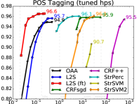
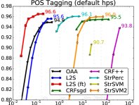
Figure 3: Training time (minutes) versus test accuracy for POS and NER. Different points correspond to different termination criteria for training. The rightmost figure use default hyperparameters and the two left figures use hyperparameters that were tuned (for accuracy) on the holdout data. Results of NER with default parameters are in the appendix. X-axis is in log scale.

We compare our system with other freely available systems/algorithms, including CRF++ [27], CRF SGD [4], Structured Perceptron [9], Structured SVM [23], Structured SVM (DEMI-DCD) [6], and an unstructured baseline predicting each label independently, using one-against-all classification [3].

For each system, we consider two situations, either the default hyperparameters or the tuned hyperparameters that achieved the best performance on holdout data. We report both conditions to give a sense of how sensitive each approach is to the setting of hyperparameters (the amount of hyperparameter tuning directly affects effective training time). We use the built-in feature template of CRF++ to generate features and use them for other systems. The templates included neighboring words and, in the case of NER, neighboring POS tags. The CRF++ templates generate $630k$ unique features for the training data. However, because L2S is also able to generate features from its own templates, we also provide results for L2S (ft) in which it uses its own feature template generation.

Training time.

In Figure 3, we show trade-offs between training time (x-axis, log scaled) and prediction accuracy (y-axis) for the aforementioned six systems. For POS tagging, the independent classifier is the fastest (trains in less than one minute) but its performance peaks at $95\%$ accuracy. Three other approaches are in roughly the same time/accuracy trade-off: L2s, L2S (ft) and Structured Perceptron. CRF SGD takes about twice as long. DEMI-DCD (taking a half hour) and CRF++ (taking over five hours) are not competitive. Structured SVM runs out of memory before achieving competitive performance (likely due to too many constraints). For NER the story is a bit different. The independent classifiers are not competitive. Here, the two variants of L2S totally dominate. In this case, Structured Perceptron is no longer competitive and is essentially dominated by CRF SGD. The only system coming close to L2S’s performance is DEMI-DCD, although it’s performance flattens out after a few minutes. The trends in the runs with default hyperparameters show similar behavior to those with tuned, though some of the competing approaches suffer significantly in prediction performance. Structured Perceptron has no hyperparameters.

Test Time.

In addition to training time, one might care about test time behavior. On NER, prediction times where $5.3k$ tokens/second (DEMI-DCD and Structured Perceptron, $20k$ (CRF SGD and Structured SVM), $100k$ (CRF++), $220k$ (L2S (ft)), and $285k$ (L2S). Although CRF SGD and Structured Perceptron fared well in terms of training time, their test-time behavior is suboptimal. When the number of labels increases from $9$ (NER) to $45$ (POS) the relative advantage of L2S increases further. The speed of L2S is about halved while for others, it is cut down by as much as a factor of $8$ due to the $O(k)$ vs $\mathcal{O}(k^{2})$ dependence on the label set size.

5.2 Dependency Parsing

To demonstrate how the credit segment compiler handles predictions with complex dependencies, we implement an arc-eager transition-based dependency parser [35]. At each state, it takes one of the four actions $\{Shift,Reduce,Left,Right\}$ based on a simple neural network with one hidden layer of size 5 and generates a dependency parse to a sentence in the end. The rollin policy is the current (learned) policy. The probability of executing the reference policy (dynamic oracle) [19] for rollout decreases over each round. We compare our model with two recent greedy transition-based parsers implemented by the original authors, the dynamic oracle parser (Dyna) [19] and the Stanford neural network parser (Snn) [8]. We also present the best results in CoNLL-X and the best published results for CTB and PTB. The performances are evaluated by unlabeled attachment scores (UAS). Punctuation is excluded.

Table 16 shows the results. Our implementation with only ~300 lines of C++ code is competitive with Dyna and Snn, which are specifically designed for parsing. Remarkably, our system achieves strong performance on CoNLL-X without tuning any hyper-parameters, even beating heavily tuned systems participating in the challenge on one dataset. The best system to date on PTB [2] uses a global normalization, more complex neural network layers and k-best POS tags. Similarly, the best system for CTB [16] uses stack LSTM architectures tailored for dependency parsing.

Parser	Ar	Bu	Ch	Cz+	Da	Du+	Ja+	Po+	Sl+	Sw	PTB	CTB
Dyna	75.3	89.8	88.7	81.5	87.9	74.2	92.1	88.9	78.5	88.9	90.3	80.0
Snn	67.4∗	88.1	87.3	78.2	83.0	75.3	89.5	83.2∗	63.6∗	85.7	91.8#	83.9#
L2S	78.2	92.0	89.8	84.8	89.8	79.2	91.8	90.6	82.2	89.7	91.9	85.1
Best	79.3	92.0	93.2	87.30	90.6	83.6	93.2	91.4	83.2	89.5	94.4#	87.2#

Table 1: UAS on PTB, CTB and CoNLL-X. Best: the best known result in CoNLL-X or the best published results (CTB, PTB) using arbitrary features and resources. See details and additional results in text and in the appendix.

5.3 Empirical evaluation of optimizations

In Section 3, we discussed two approaches for computational improvements. Memoization avoids re-predicting on the same input multiple times while path collapse stops rollouts at a particular point in time. The effect of the different optimizations depends greatly on the underlying learning algorithm. For example, DAgger does not do rollouts at all, so no efficiency is gained by either optimization. The affected algorithms are LOLS (with mixed rollouts) and Searn.

NER POS LOLS Searn LOLS Searn No Opts 96s 123s 3739s 4255s Mem. 75s 85s 1142s 1215s Col.@4+Mem. 71s 75s 1059s 1104s Col.@2+Mem. 69s 71s 1038s 1074s

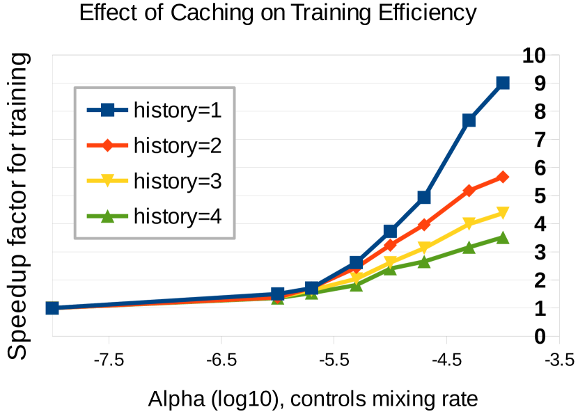
Figure 4: The table on the left shows the effect of Collapse (Col) and Memorization (Mem.). The figure on the right shows the speed-up obtained for different historical lengths and mixing rate of rollout policy. Large $\alpha$ corresponds to more prediction required when training the model.

Figure 4 shows the effect of these optimizations on the best NER and POS systems we trained without using external resources. In the left table, we can see that memoization alone reduces overall training runtime by about $25\%$ on NER and about $70\%$ on POS, essentially because the overhead for the classifier on POS tagging is so much higher (45 labels versus 9). When rollouts are terminated early, the speed increases are much more modest, essentially because memoization is already accounting for much of these gains. In all cases, the final performance of the predictors is within statistical significance of each other (p-value of 0.95, paired sign test), except for Collapse@2+Memoization on NER, where the performance decrease is only insignificant at the 0.90 level. The right figure demonstrates that when $\alpha$ increases, more prediction is required during the training time, and the speedup increases from a factor of 1 (no change) to a factor of as much as 9. However, as the history length increases, the speedup is more modest due to low cache hits.

6 Related Work

Several algorithms are similar to learning to search approaches, including the incremental structured perceptron [10, 22], HC-Search [13, 14], and others [12, 38, 45, 48, 49]. Some fit this framework.

Probabilistic programming [21] has been an active area of research. These approaches have a different goal: Providing a flexible framework for specifying graphical models and performing inference in those models. The credit assignment compiler instead allows a developer to learn to make coherent decisions for joint prediction (“learning to search”). We also differ by not designing a new programming language. Instead, we have a two-function library which makes adoption and integration into existing code bases much easier.

The closest work to ours is Factorie [31]. Factorie is essentially an embedded language for writing factor graphs compiled into Scala to run efficiently. Factorie acts more like a library than a language although it’s abstraction is still factor graph distributions. Similarly, Infer.NET [33], Markov Logic Networks (MNLs)  [39], and Probabilistic Soft Logic (PSL) [25] concisely construct and use probabilistic graphical models. BLOG [32] falls in the same category, though with a very different focus. Similarly, Dyna [17] is a related declarative language for specifying probabilistic dynamic programs, and Saul [26] is a declarative language embedded in Scala that deals with joint prediction via integer linear programming. All of these examples have picked particular aspects of the probabilistic modeling framework to focus on. Beyond these examples, there are several approaches that essentially “reinvent” an existing programming language to support probabilistic reasoning at the first order level. IBAL [36] derives from O’Caml; Church [20] derives from LISP. IBAL uses a (highly optimized) form of variable elimination for inference that takes strong advantage of the structure of the program; Church uses MCMC techniques, coupled with a different type of structural reasoning to improve efficiency.

Appendix A Example TDOLR programs

In this section, a few other TDOLR programs which illustrate the ease and flexibility of programming.

Algorithm 4 is for a sequential detection task where the goal is to detect whether or not a sequence contains some rare element. This illustrates outputs of lengths other than the number of examples, explicit loss functions.

Algorithm 4 Sequential_Detection_RUN(examples as $X$, false_negative_loss)

1:  Let max_value = 1

2:  for $i$ $={\color[rgb]{0.2,0.2,0.2}\textit{1}}$ to len(examples) do

3:     max_value $\leftarrow$ max(max_value, examples[i].label)

4:  Let max_prediction = 1

5:  for $i$ $={\color[rgb]{0.2,0.2,0.2}\textit{1}}$ to len(examples) do

6:     max_prediction $\leftarrow$ max(max_prediction, predict($x$=examples[i], $y$=examples[i].label)) // maintain max

7:  if max_label > max_prediction then

8:     loss(false_negative_loss) // The loss is asymmetric

9:  else

10:     if max_label < max_prediction then

11:        loss(1)

12:     else

13:        loss(0)

14:  if output.good then

15:     output << max_prediction// if we should generate output, append our prediction

In Algorithm 5, we show an implementation of a shift-reduce dependency parser for natural language. We discuss each subcomponent below. The detailed introduction to dependency parsing is provided in the next section.

• GetValidAction returns valid actions that can be taken by the current configuration.

• GetFeat extracts features based on the current configuration. A detailed list of our features is in the supplementary material.

• GetGoldAction implements the dynamic oracle described in [19]. The dynamic oracle returns the optimal action in any state that leads to a reachable end state with the minimal loss.

• Predict is a library call implemented in the L2S system. Given training samples, L2S can learn the policy automatically. In the test phase, it returns a predicted action leading to an end state with small structured loss.

• Trans implements the hybrid-arc transition system described above.

• Loss returns the number of words whose parents are wrong. It has no effect in the test phase.

Algorithm 5 RunParser(sentence as $X$)

1:  stack $S$ $\leftarrow$ {Root}

2:  buffer $B$ $\leftarrow$ [words in sentence]

3:  arcs $A$ $\leftarrow$ $\emptyset$

4:  while  $B\neq\emptyset$ or $|S|>1$ do

5:     ValidActs $\leftarrow$ GetValidActions($S,B$)

6:     features $\leftarrow$ GetFeat($S,B,A$)

7:     ref $\leftarrow$ GetGoldAction($S,B$)

8:     action $\leftarrow$ predict($x$=features, $y$=ref, ValidActs)

9:     $S,B,A$ $\leftarrow$ Trans($S,B,A$, action)

10:  loss($A[w]$ $\neq$ $A^{*}[w]$, $\forall w\in$ sentence)

11:  return output

We show that this parser achieves strong results across ten languages from the CoNLL-X challenge and performs well on two standard evaluation data sets, and requires only about $300$ lines of readable C++ code.

Finally, Algorithm 6 provides an implementation for jointly assigning types to name entities in a sentence and recognizing relations between them [43]. Besides features used for predicting entity and relation types. We also consider constraints that ensure the entity-type assignments and relation-type assignments are compatible with each other. For example, the first argument of the work_for relation need to be tagged as person, and the second argument has to be an organization.

Algorithm 6 Entity_Relation_RUN(sent as $X$)

1:  output $\leftarrow$ Initialize_structure()

2:  K $\leftarrow$ Number_of_entities(sent)

3:  for n = 1 to K do

4:     ref $\leftarrow$ sent.entity_type[n]

5:     output.entity_type[n] $\leftarrow$ predict($x$=sent.entity[i], $y$=ref, tag=n

6:     loss(output.entity_type[n] $\neq$ sent.entity_type[n].true_label)

7:  for n = 1 to K-1 do

8:     for m = n+1 to K) do

9:        ref $\leftarrow$ sent.relation_type[n,m].true_label

10:        valid_relations $\leftarrow$ Find_valid_relations(output.entity_type[n], output.entity_type[m])

11:        output.relation_type $\leftarrow$ predict($x$=sent.relation[n,m], $y$=ref, tag=K*(n+1)+m, valid_labels=valid_relations, condition=[n,m])

12:        loss(output.relation_type[n,m] $\neq$ sent.entity_type[n,m].true_label )

13:  return output

Action	Configuration
	Stack	Buffer	Arcs
	[Root]	[Flying planes can be dangerous]	{}
Shift	[Root Flying]	[planes can be dangerous]	{}
Reduce-left	[Root]	[planes can be dangerous]	{(planes, Flying)}
Shift	[Root planes]	[can be dangerous]	{(planes, Flying)}
Reduce-left	[Root]	[can be dangerous]	{(planes, Flying), (can, planes)}
Shift	[Root can]	[be dangerous]	{(planes, Flying), (can, planes)}
Shift	[Root can be]	[dangerous]	{(planes, Flying), (can, planes)}
Shift	[Root can be dangerous]	[]	{(planes, Flying), (can, planes)}
Reduce-Right	[Root can be]	[]	{(planes, Flying), (can, planes), (be, dangerous)}
Reduce-Right	[Root can]	[]	{(planes, Flying), (can, planes), (be, dangerous), (can, be)}
Reduce-Right	[Root]	[]	{(planes, Flying), (can, planes), (be, dangerous), (can, be), (Root, can)}

Parse tree derived by the above parser	Gold parse tree

Figure 5: An illustrative example of an arc-hybrid transition parser. The above table show the actions taken and the intermediate configurations generated by a parser. The parse tree derived by the parser is in the bottom left, and the gold parse tree is the bottom right. The distance between these two trees is 2.

Appendix B Dependency Parsing

In the following, we provide a brief overview of transition-based dependency parsing. A transition-based dependency parser takes a sequence of actions and parses a sentence from left to right by maintaining a stack $S$, a buffer $B$, and a set of dependency arcs $A$. The stack maintains partial parses, the buffer stores the words to be parsed, and $A$ keeps the arcs that have been generated so far. The configuration of the parser at each stage can be defined by a triple $(S,B,A)$. For the ease of notation, we use $w_{p}$ to represent the leftmost word in the buffer and use $s_{1}$ and $s_{2}$ to denote the top and the second top words in the stack. A dependency arc $(w_{h},w_{m})$ is a directed edge that indicates word $w_{h}$ is the parent of word $w_{m}$. When the parser terminates, the arcs in $A$ form a projective dependency tree. We assume that each word only has one parent in the derived dependency parse tree, and use $A[w_{m}]$ to denote the parent of word $w_{m}$. For labeled dependency parsing, we further assign a tag to each arc representing the dependency type between the head and the modifier. For simplicity, we assume an unlabeled parser in the following description. The extension from an unlabeled parser to a labeled parser is straightforward, and is discussed at the end of this section.

Algorithm 7 Trans($S$, $B$, $A$, action)

1:  Let $w_{p}$ be the leftmost element in $B$

2:  if action = Shift then

3:     $S$.push($w_{p}$)

4:     remove $w_{p}$ from $B$

5:  else if action= Reduce-Left then

6:     top $\leftarrow$ $S$.pop()

7:     $A$ $\leftarrow$ $A\cup$ ($w_{p}$,top)

8:  else if action = Reduce-Right then

9:     top $\leftarrow$ $S$.pop()

10:     $A$ $\leftarrow$ $A\cup$ ($S$.top(), top)

11:  return $S,B,A$

In the following, we describe an arc-hybrid transition system due to its simplicity. The arc-eager system used in the experiments share the same spirit. In the initial configuration, the buffer $B$ contains all the words in the sentence, a dummy root node is pushed in the stack $S$, and the set of arcs $A$ is empty. The root node cannot be popped out at anytime during parsing. The system then takes a sequence of actions until the buffer is empty and the stack contains only the root node (i.e., $|B|=0$ and $S=\{\textbf{Root}\}$). When the process terminates, a parse tree is derived. At each state, the system can take one of the following actions:

1. Shift: push $w_{p}$ to $S$ and move $p$ to the next word. (Valid when $|B|>0$).

2. Reduce-left: add an arc ($w_{p}$, $s_{1}$) to $A$ and pop $s_{1}$. (Valid when $|B|>0$ and $|S|>1$).

3. Reduce-right: add an arc ($s_{2}$, $s_{1}$) to $A$ and pop $s_{1}$. (Valid when $|S|>1$).

Algorithm 7 shows the execution of these actions during parsing, and Figure 5 demonstrates an example of transition-based dependency parsing.

Appendix C Additional Experiment Results

C.1 Sequential Tagging

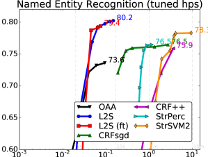
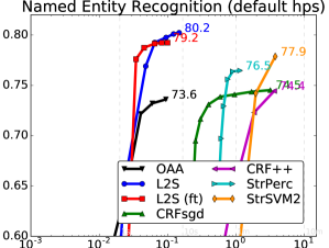
Figure 6: Training time versus evaluation accuracy for part of speech tagging (left) and named entity recognition (right). X-axis is in log scale. Different points correspond to different termination criteria for training. Top figures use hyperparameters that were tuned (for accuracy) on the holdout data. (Note: lines are curved due to log scale x-axis.)

In Figure 6, we enlarge the figures in 3 and provide the results of NER with default parameters.

C.2 Dependency Parsing

Parser	Ar	Bu	Ch	Cz+	Da	Du+	Ja+	Po+	Sl+	Sw	PTB	CTB
	UAS
Dyna	75.3	89.8	88.7	81.5	87.9	74.2	92.1	88.9	78.5	88.9	90.3	80.0
Snn	67.4∗	88.1	87.3	78.2	83.0	75.3	89.5	83.2∗	63.6∗	85.7	91.8#	83.9#
L2SO	75.3	89.5	87.4	81.1	86.0	75.3	90.4	88.4	78.5	89.9	91.9	85.1
L2S	78.2	92.0	89.8	84.8	89.8	79.2	91.8	90.6	82.2	89.7	91.9	85.1
Best	79.3	92.0	93.2	87.30	90.6	83.6	93.2	91.4	83.2	89.5	94.4#	87.2#
	LAS
Dyna	64.3	85.0	84.6	74.1	82.5	70.3	90.6	85.0	68.5	83.5	88.1	78.8
Snn	51.7∗	84.0	82.7	77.4	72.0	89.1	87.4 ∗	77.9 ∗	51.1∗	80.1	89.6#	82.4#
L2SO	65.1	85.0	80.8	74.5	81.0	72.1	88.4	84.4	69.4	85.2	89.7	83.6
L2S	68.2	88.2	87.1	79.6	84.9	75.8	89.7	87.8	74.0	84.9	89.7	83.6
Best	66.9	87.6	90.0	80.2	84.8	79.2	91.7	87.6	73.4∗	84.6	92.55#	85.7#

Table 2: Accuracy on PTB, CTB and CoNLL-X. Best: best results from the shared task. Best: the best results reported in CoNLL-X (may come from different participants) and the best published results (CTB,PTB). L2S^O, Dyna, Snn use only features generated by word and POS tags, while L2S and the models in CoNLL-X use additional morphologic features. L2S models use Brown cluster for PTB, Dyna and the Best use word embedding features generated from unsupervised text corpus with billion words. The Best models also used word embedding features for $CTB$.

Parser	Ar	Bu	Ch	Cz+	Da	Du+	Ja+	Po+	Sl+	Sw	PTB	CTB
Dyna				r		r	r	r	r		T	T
Snn	r’			r		r	r	r’	r’		T	T
L2SO				r		r	r	r	r		T	T
L2S	M	M	M	rM	M	rM	rM	rM	rM	M	ET	T
Best	TM	TM	TM	TM	TM	TM	TM	TM	TM	TM	ET	ET

Table 3: T: tuned hyper-parameters, M: use morphological features, E: use word embedding or word clustering, r: language structure assumption that may degrades the performance (the nature of transition-based model), r’: strong language structure assumption (only one head) that severely degrades the performance. Accuracy on PTB, CTB and CoNLL-X. Best: best results from the shared

Table 20 show the complete experiment results for dependency parsing. The system is evaluated on both unlabeled attachment score (UAS) and labeled attachment score. Again, conducting fair comparisons across different systems is difficult because different systems use different sets of features and different assumptions about the structure of languages. Table 3 summarizes the differences.

Appendix D Experiment details

D.1 Datasets and Tasks

	Training					Holdout		Test
	Sents	Toks	Labels	Features	Unique Fts	Sents	Toks	Sents	Toks
POS	38k	912k	45	13,685k	629k	5.5k	132k	5.5k	130k
NER	15k	205k	7	8,592k	347k	3.5k	52k	3.6k	47k

Table 4: Basic statistics about the data sets used for part of speech (POS) tagging and named entity recognition (NER).

POS

NNP NNP , CD NNS JJ , MD VB DT NN IN DT JJ NN Pierre Vinken , 61 years old , will join the board as a nonexecutive director …

NER

${\color[rgb]{0.0,0.0,0.5}\overbrace{\textnormal{{\color[rgb]{0,0,0}Germany}}}^{\textsf{LOC}}}$ ’s rep to the ${\color[rgb]{0.0,0.0,0.5}\overbrace{\textnormal{{\color[rgb]{0,0,0}European Union}}}^{\textsf{ORG}}}$ ’s committee ${\color[rgb]{0.0,0.0,0.5}\overbrace{\textnormal{{\color[rgb]{0,0,0}Werner Zwingmann}}}^{\textsf{PER}}}$ said …

Figure 7: Example inputs (below, black) and desired outputs (above, blue) for part of speech tagging task, named entity recognition task, and entity-relation recognition task.

We conduct experiments based on two variants of the sequence labeling problem (Algorithm 1) The first is a pure sequence labeling problem: Part of Speech tagging based on data from the Wall Street Journal portion of the Penn Treebank. The second is a sequence chunking problem: named entity recognition using data from the CoNLL 2003 dataset. See Figure 7 for example inputs and outputs for these tasks.

Part of speech tagging for English is based on the Penn Treebank tagset that includes $45$ discrete labels. The accuracy reported represents number of tokens tagged correctly. This is a pure sequence labeling task. Named entity recognition for English is based on the CoNLL 2003 dataset that includes four entity types: Person, Organization, Location and Miscellaneous. We use the standard evaluation metric to report performance as macro-averaged F-measure. In order to cast this chunking task as a sequence labeling task, we use the standard Begin-In-Out (BIO) encoding, though some results suggest other encodings may be preferable [37] (we tried BILOU and our accuracies decreased). The example sentence from Figure 7 in this encoding is:

${\color[rgb]{0.0,0.0,0.5}\overbrace{\textnormal{{\color[rgb]{0,0,0}Germany}}}^{\textsf{LOC}}}$	’s	rep	to	the	${\color[rgb]{0.0,0.0,0.5}\overbrace{\textnormal{{\color[rgb]{0,0,0}European Union}}}^{\textsf{ORG}}}$	’s	committee	${\color[rgb]{0.0,0.0,0.5}\overbrace{\textnormal{{\color[rgb]{0,0,0}Werner Zwingmann}}}^{\textsf{PER}}}$	said	…
B-LOC	O	O	O	O	B-ORG       I-ORG	O	O	B-PER          I-PER	O

Dependency parser is test on the English Penn Treebank (PTB) and the CoNLL-X datasets for 9 other languages, including Arabic, Bulgarian, Chinese, Danish, Dutch, Japanese, Portuguese, Slovene and Swedish. For PTB, we convert the constituency trees to dependencies by the Stanford parser 3.3.0. We follow the standard split: sections 2 to 21 for training, section 22 for development and section 23 for testing. The POS tags in the evaluation data is assigned by the Stanford POS tagger, which has an accuracy of 97.2% on the PTB test set. For CoNLL-X, we use the given train/test splits and reserve the last 10% of training data for development if needed. The gold POS tags given in the CoNLL-X datasets are used. The CTB is prepared following the instructions in [8].

D.2 Methodology

Comparing different systems is challenging because one wishes to hold constant as many variables as possible. In particular, we want to control for both features and hyperparameters. In general, if a methodological decision cannot be made “fairly,” we made it in favor of competing approaches.

To control for features, for the two sequential tagging tasks (POS and NER), we use the built-in feature template approach of CRF++ (duplicated in CRF SGD) to generate features. The other approaches (Structured SVM, VW Search and VW Classification) all use the features generated (offline) by CRF++. For each task, we tested six feature templates and picked the one with best development performance using CRF++. The templates included neighboring words and, in the case of NER, neighboring POS tags. However, because VW Search is also able to generate features from its own templates, we also provide results for VW Search (own fts) in which it uses its own, internal, feature template generation, which were tuned to maximize it’s holdout performance on the most time-consuming run (4 passes) and include neighboring words (and POS tags, for NER) and word prefixes/suffixes. In all cases we use first order Markov dependencies, which lessens the speed advantage of search based structured prediction.

To control for hyperparameters, we first separated each system’s hyperparameters into two sets: (1) those that affect termination condition and (2) those that otherwise affect model performance. When available, we tune hyperparameters for (a) learning rate and (b) regularization strength. Additionally, we vary the termination conditions to sweep across different amounts of time spent training. For each termination condition, we can compute results using either the default hyperparameters or the tuned hyperparameters that achieved best performance on holdout data. We report both conditions to give a sense of how sensitive each approach is to the setting of hyperparameters (the amount of hyperparameter tuning directly affects effective training time).

One final confounding issue is that of parallelization. Of the baseline approaches, only CRF++ supports parallelization via multiple threads at training time. In our reported results, CRF++’s time is the total CPU time (i.e., effectively using only one thread). Experimentally, we found that wall clock time could be decreased by a factor of $1.8$ by using $2$ threads, a factor of $3$ using $4$ threads, and a (plateaued) factor of $4$ using $8$ threads. This should be kept in mind when interpreting results. DEMI-DCD (for structured SVMs) also must use multiple threads. To be as fair as possible, we used $2$ threads. Likewise, it can be sped up more using more threads [6]. VW (Search and Classification) can also easily be parallelized using AllReduce [1]. We do not conduct experiments with this option here because none of our training times warranted parallelization (a few minutes to train, max).

For dependency parsing, we fixed the hyper-parameters when test on CoNLL-X. For CTB and PTB, we tune the size of beam in beam search and the history length of predictions. For PTB, we further use dictionary features from Brown cluster.

D.3 Hardware Used

All timing results were obtained on the same machine with the following configuration. Nothing else was run on this machine concurrently:

%   2 * Intel(R) Core(TM)2 Duo CPU E8500 @ 3.16GHz
  6144 KB cache
  8 GB RAM, 4 GB Swap
  Red Hat Enterprise Linux Workstation release 6.5 (Santiago)
  Linux 2.6.32-431.17.1.el6.x86_64 #1 SMP
    from Fri Apr 11 17:27:00 EDT 2014 x86_64 x86_64 x86_64 GNU/Linux

D.4 Software Used

The precise software versions used for comparison are:

• The popular CRF++ toolkit [27] for conditional random fields [28].

• A stochastic gradient descent conditional random field package [4].

• An implementation of the structured perceptron [9] due to [6].

• ] The cutting-plane implementation [23] of the structured SVMs [47] for “HMM” problems.

• A multicore algorithm for optimizing structured SVMs called DEcoupled Model-update and Inference with Dual Coordinate Descent.

• Our approach is implemented in the Vowpal Wabbit [29] toolkit on top of a cost-sensitive classifier [3] that reduces to regression trained with an online rule incorporating AdaGrad [15], per-feature normalized updates [42], and importance invariant updates [24].

• An unstructured baseline that predicts each label independently, using one-against-all multiclass classification [3].

• latest Vowpal Wabbit version (May 2016) commit 2dfb1225c8b89c14552932161b95237fc90b636c

• CRF++ version 0.58

• crfsgd version 2.0

• svm_hmm_learn version 3.10, 14.08.08
  includes SVM-struct V3.10 for learning complex outputs, 14.08.08
  includes SVM-light V6.20 quadratic optimizer, 14.08.08

• Illinois-SL version 0.2.2

D.5 Hyperparameters Tuned

The hyperparameters tuned and the values we considered for each system are:

CRF++

%     termination parameters:
      number of passes (--max_iter)     { 2, 4, 8, 16, 32, 64, 128 }
      termination criteria (--eta)      0.000000000001 (to prevent termination)

    tuned hyperparameters (default is *):
      learning algorithm (--algorithm)  { CRF*, MIRA }
      cost parameter (--cost)           { 0.0625, 0.125, 0.25, 0.5, 1*, 2, 4, 8, 16 }

CRF SGD

%     termination parameters:
      number of passes (-r)             { 1, 2, 4, 8, 16, 32, 64, 128 }

    tuned hyperparameters (default is *):
      regularization parameter (-c)     { 0.0625, 0.125, 0.25, 0.5, 1*, 2, 4, 8, 16 }
      learning rate (-s)                { auto*, 0.1, 0.2, 0.5, 1, 2, 5 }

Structured SVM

%     termination parameters:
      epsilon tolerance (-e)            { 4, 2, 1, 0.5, 0.1, 0.05, 0.01, 0.005, 0.001 }

    tuned hyperparameters (default is *):
      regularization parameter (-c)     { 0.0625, 0.125, 0.25, 0.5, 1*, 2, 4, 8, 16 }

Structured Perceptron

%     termination parameters:
      number of passes (MAX_NUM_ITER)   { 1, 2, 4, 8, 16, 32, 64, 128 }

    tuned hyperparameters (default is *):
      NONE

Structured SVM (DEMI-DCD)

%     termination parameters:
      number of passes (MAX_NUM_ITER)   { 1, 2, 4, 8, 16, 32, 64, 128 }

    tuned hyperparameters (default is *):
      regularization (C_FOR_STRUCTURE)  { 0.01, 0.05, 0.1*, 0.5, 1.0 }

L2S

    termination parameters:
      number of passes (--passes)       { 0.01, 0.02, 0.05, 0.1, 0.2, 0.5, 1, 2, 4 }
      (note: a number of passes < 1 means that we perform one full pass, but
       _subsample_ the training positions for each sequence at the given rate)

    tuned hyperparameters (default is *):
      base classifier                   { csoaa*}
      interpolation rate                10^{-10, -9, -8, -7, -6 }

VW Classifier

    termination parameters:
      number of passes (--passes)       { 1, 2, 4 }

    tuned hyperparameters (default is *):
      learning rate (-l)                { 0.25, 0.5*, 1.0 }

Appendix E Templates Used

For part of speech tagging (CRF++):

    U00:%x[-2,0]
    U01:%x[-1,0]
    U02:%x[0,0]
    U03:%x[1,0]
    U04:%x[2,0]

For named entity recognition (CRF++):

    U00:%x[-2,0]
    U01:%x[-1,0]
    U02:%x[0,0]
    U03:%x[1,0]
    U04:%x[2,0]

    U10:%x[-2,1]
    U11:%x[-1,1]
    U12:%x[0,1]
    U13:%x[1,1]
    U14:%x[2,1]

    U15:%x[-2,1]/%x[-1,1]
    U16:%x[-1,1]/%x[0,1]
    U17:%x[0,1]/%x[1,1]
    U18:%x[1,1]/%x[2,1]

(where words are in position 0 and POS is in 1)

Additional features for L2S (ft) on POS Tagging:

  -- the left and the right tokens of each word
  -- the first and the last 2 characters for each token

For L2S (ft) on NER:

  -- the left and the right two tokens of each word
  -- the POS tags of the left and the right tokens for each word
  -- the last charaster for each token

References

- [1] Alekh Agarwal, Olivier Chapelle, Miroslav Dudík, and John Langford. A reliable effective terascale linear learning system. arXiv preprint arXiv:1110.4198, 2011.
- [2] Daniel Andor, Chris Alberti, David Weiss, Aliaksei Severyn, Alessandro Presta, Kuzman Ganchev, Slav Petrov, and Michael Collins. Globally normalized transition-based neural networks. Arxiv, 2016.
- [3] Alina Beygelzimer, Varsha Dani, Tom Hayes, John Langford, and Bianca Zadrozny. Error limiting reductions between classification tasks. In ICML, pages 49–56, 2005.
- [4] Leon Bottou. crfsgd project, 2011. http://leon.bottou.org/projects/sgd.
- [5] Kai-Wei Chang, Akshay Krishnamurthy, Alekh Agarwal, Hal Daumé III, and John Langford. Learning to search better than your teacher. In ICML, 2015.
- [6] Kai-Wei Chang, Vivek Srikumar, and Dan Roth. Multi-core structural SVM training. In ECML, 2013.
- [7] Kai-Wei Chang, Shyam Upadhyay, Ming-Wei Chang, Vivek Srikumar, and Dan Roth. Illinoissl: A JAVA library for structured prediction. Arxiv, 2015.
- [8] Danqi Chen and Christopher Manning. A fast and accurate dependency parser using neural networks. In EMNLP, pages 740–750, 2014.
- [9] Michael Collins. Discriminative training methods for hidden Markov models: Theory and experiments with perceptron algorithms. In EMNLP, 2002.
- [10] Michael Collins and Brian Roark. Incremental parsing with the perceptron algorithm. In ACL, 2004.
- [11] Hal Daumé III, John Langford, and Daniel Marcu. Search-based structured prediction. Machine Learning Journal, 2009.
- [12] Hal Daumé III and Daniel Marcu. Learning as search optimization: Approximate large margin methods for structured prediction. In ICML, 2005.
- [13] Janardhan Rao Doppa, Alan Fern, and Prasad Tadepalli. Output space search for structured prediction. In ICML, 2012.
- [14] Janardhan Rao Doppa, Alan Fern, and Prasad Tadepalli. HC-Search: A learning framework for search-based structured prediction. JAIR, 50, 2014.
- [15] John Duchi, Elad Hazan, and Yoram Singer. Adaptive subgradient methods for online learning and stochastic optimization. JMLR, 12:2121–2159, 2011.
- [16] Chris Dyer, Miguel Ballesteros, Wang Ling, Austin Matthews, and Noah A. Smith. Transition-based dependency parsing with stack long short-term memory. In ACL, 2015.
- [17] Jason Eisner, Eric Goldlust, and Noah A. Smith. Compiling comp ling: Practical weighted dynamic programming and the dyna language. In EMNLP, 2005.
- [18] Ulrich Germann, Mike Jahr, Kevin Knight, Daniel Marcu, and Kenji Yamada. Fast decoding and optimal decoding for machine translation. Artificial Intelligence, 154(1-2):127–143, 2003.
- [19] Yoav Goldberg and Joakim Nivre. Training deterministic parsers with non-deterministic oracles. Transactions of the ACL, 1, 2013.
- [20] Noah Goodman, Vikash Mansinghka, Daniel Roy, Keith Bonawitz, and Josh Tenenbaum. Church: a language for generative models. In UAI, 2008.
- [21] Andrew D. Gordon, Thomas A. Henzinger, Aditya V. Nori, and Sriram K. Rajamani. Probabilistic programming. In International Conference on Software Engineering (ICSE, FOSE track), 2014.
- [22] Liang Huang, Suphan Fayong, and Yang Guo. Structured perceptron with inexact search. In NAACL, 2012.
- [23] Thorsten Joachims, Thomas Finley, and Chun-Nam Yu. Cutting-plane training of structural SVMs. Machine Learning Journal, 2009.
- [24] Nikos Karampatziakis and John Langford. Online importance weight aware updates. In UAI, 2011.
- [25] Angelika Kimmig, Stephen Bach, Matthias Broecheler, Bert Huang, and Lise Getoor. A short introduction to probabilistic soft logic. In NIPS Workshop on Probabilistic Programming, 2012.
- [26] Parisa Kordjamshidi, Dan Roth, and Hao Wu. Saul: Towards declarative learning based programming. In IJCAI, 2015.
- [27] Taku Kudo. CRF++ project, 2005. http://crfpp.googlecode.com.
- [28] John Lafferty, Andrew McCallum, and Fernando Pereira. Conditional random fields: Probabilistic models for segmenting and labeling sequence data. In ICML, pages 282–289, 2001.
- [29] John Langford, Alex Strehl, and Lihong Li. Vowpal wabbit, 2007. http://hunch.net/~vw.
- [30] Andrew McCallum, Dayne Freitag, and Fernando Pereira. Maximum entropy Markov models for information extraction and segmentation. In ICML, 2000.
- [31] Andrew McCallum, Karl Schultz, and Sameer Singh. FACTORIE: probabilistic programming via imperatively defined factor graphs. In NIPS, 2009.
- [32] Brian Milch, Bhaskara Marthi, Stuart Russell, David Sontag, Daniel L Ong, and Andrey Kolobov. BLOG: probabilistic models with unknown objects. Statistical relational learning, 2007.
- [33] Tom Minka, John Winn, John Guiver, and David Knowles. Infer .net 2.4, 2010. microsoft research cambridge, 2010.
- [34] Andrew Ng and Michael Jordan. PEGASUS: A policy search method for large MDPs and POMDPs. In UAI, pages 406–415, 2000.
- [35] Joakim Nivre. An efficient algorithm for projective dependency parsing. In IWPT, pages 149–160, 2003.
- [36] Avi Pfeffer. Ibal: A probabilistic rational programming language. In IJCAI, 2001.
- [37] Lev Ratinov and Dan Roth. Design challenges and misconceptions in named entity recognition. In CoNLL, 2009.
- [38] Nathan Ratliff, David Bradley, J. Andrew Bagnell, and Joel Chestnutt. Boosting structured prediction for imitation learning. In NIPS, 2007.
- [39] Matthew Richardson and Pedro Domingos. Markov logic networks. Machine learning, 62(1-2), 2006.
- [40] Stéphane Ross and J. Andrew Bagnell. Reinforcement and imitation learning via interactive no-regret learning. arXiv:1406.5979, 2014.
- [41] Stephane Ross, Geoff J. Gordon, and J. Andrew Bagnell. A reduction of imitation learning and structured prediction to no-regret online learning. In AI-Stats, 2011.
- [42] Stéphane Ross, Paul Mineiro, and John Langford. Normalized online learning. In UAI, 2013.
- [43] Dan Roth and Scott Wen-Tau Yih. Global inference for entity and relation identification via a linear programming formulation. In Introduction to Statistical Relational Learning. MIT Press, 2007.
- [44] Wee Meng Soon, Hwee Tou Ng, and Daniel Chung Yong Lim. A machine learning approach to coreference resolution of noun phrases. Computational Linguistics, 27(4):521 – 544, 2001.
- [45] Umar Syed and Robert E. Schapire. A reduction from apprenticeship learning to classification. In NIPS, 2011.
- [46] Ben Taskar, Carlos Guestrin, and Daphne Koller. Max-margin Markov networks. In NIPS, 2003.
- [47] Ioannis Tsochantaridis, Thomas Hofmann, Thorsten Joachims, and Yasmine Altun. Support vector machine learning for interdependent and structured output spaces. In ICML, 2004.
- [48] Yuehua Xu and Alan Fern. On learning linear ranking functions for beam search. In ICML, pages 1047–1054, 2007.
- [49] Yuehua Xu, Alan Fern, and Sung Wook Yoon. Discriminative learning of beam-search heuristics for planning. In IJCAI, pages 2041–2046, 2007.