Periodic massloss from viscous accretion flows around black holes

Abstract

We investigate the behaviour of low angular momentum viscous accretion flows around black holes using Smooth Particle Hydrodynamics (SPH) method. Earlier, it has been observed that in a significant part of the energy and angular momentum parameter space, rotating transonic accretion flow undergoes shock transition before entering in to the black hole and a part of the post-shock matter is ejected as bipolar outflows, which are supposed to be the precursor of relativistic jets. In this work, we simulate accretion flows having injection parameters from the inviscid shock parameter space, and study the response of viscosity on them. With the increase of viscosity, shock becomes time dependent and starts to oscillate when the viscosity parameter crosses its critical value. As a result, the in falling matter inside the post-shock region exhibits quasi-periodic variations and causes periodic ejection of matter from the inner disc as outflows. In addition, the same hot and dense post-shock matter emits high energy radiation and the emanating photon flux also modulates quasi-periodically. Assuming a ten solar mass black hole, the corresponding power density spectrum peaks at the fundamental frequency of few Hz followed by multiple harmonics. This feature is very common in several outbursting black hole candidates. We discuss the implications of such periodic variations.

1 Introduction

Luminosities and spectra emanating from the microquasars and AGNs are best explained by the gravitational energy released due to accretion onto compact objects such as black holes. However, it has been established in recent years, that black hole candidates, be it stellar mass or super massive, emits powerful collimated outflows or jets (Livio, 1999). Since black holes do not have intrinsic atmosphere or hard surface, these jets have to be generated from the accretion disc itself. In a very interesting paper, Junor et al. (1999) had shown that jets originate from around a region less than $100r_{g}$ ($r_{g}{\equiv}$ Schwarzschild radius) across the central object of the nearby active galaxy M87. Since the typical timescale of an AGN or a microquasar scales with mass, temporal behaviour of black hole candidates is studied with microquasars (McHardy et al., 2006). After investigating the connection between accretion and ejection in ten microquasars, Gallo et al. (2003) concluded that mildly relativistic, quasi steady jets are generally ejected in the low hard spectral states (i.e., when electromagnetic spectra peak in the high energy power-law frequency range) of the accretion disc. It was also shown that jets tend to get stronger as the microquasar moves to the intermediate hard states, and truly relativistic ejections are observed during hard-intermediate to soft-intermediate transition, after which the microquasar enters canonical high soft state (i.e., when spectra peak in the thermal low energy range), which shows no jet activity (Rushton et al., 2010; Miller-Jones et al., 2012). All these evidences suggest that the generation or quenching of jets do depend on various states of the accretion disc, and that, the jet formation mechanism is linked with the processes that dominate at distances relatively closer to the black hole.

It is well known that, spectra from microquasar change states between, the low hard state (LH) and high soft state (HS), through a series of intermediate states. Interestingly, the hard power-law photons exhibit a quasi-periodic oscillations (QPO). The QPOs evolve along with the spectral states of the accretion disc, starting with low frequencies in LH, increasing as the luminosity increases, and reaches highest value before disappearing in the HS state (Chakrabarti et al., 2008; Shaposhnikov & Titarchuk, 2009; Nandi et al., 2012, 2013). Interestingly, although QPO frequency increases as the accretion disc moves from LH to intermediate states, but no QPO was detected during ejection of relativistic jets (Nandi et al., 2013; Radhika & Nandi, 2013) which suggests that, probably the part of the disc responsible for QPO is entirely ejected as relativistic jets. This conversely also suggests that, the inner part of the disc is responsible for QPOs and is also the base of the jet. Accretion disc models which are invoked to explain the accretion-ejection phenomena around black hole candidates, should at least address the connection between spectral states, QPO evolution and the evolution of jets, apart from matching the luminosities radiated by AGNs and microquasars.

There are various accretion disc models in the literature. We know that, matter crosses the horizon with the speed of light ($c$) and circular orbits cannot exist within the marginally stable orbit ($3r_{g}$). So the inner boundary condition for accretion onto black hole is necessarily transonic, as well as, sub-Keplerian, which implies that advection should be significant at least close to the horizon. The very first model of accretion onto black holes was of course radial inflow of matter, which was basically the general relativistic version of the Bondi solutions (Bondi, 1952; Michel, 1972). However, the infall time scale of radial accretion onto black holes is short, and therefore has very little time to produce the huge luminosities observed from AGNs and microquasars (Shapiro, 1973). On the other hand, Shakura & Sunyaev (1973) considered a geometrically thin but optically thick accretion disc characterized by negligible advection, but by virtue of possessing Keplerian angular momentum distribution, the disc was rotation dominated. This disc model was radiatively efficient and produced the multi-coloured blackbody part of the spectra or the ‘blue bump’ radiated by the AGNs. However, the presence of hard power-law tail in the spectra of the black hole candidates indicated the necessity of a hot Comptonizing cloud, which was neither present in Keplerian disc nor its origin could be identified in any self-consistent manner from such a disc. Therefore, models with advection gained importance. Theoretically, it was shown that in a significant range of energy and angular momentum, multiple sonic points may exist for rotating, transonic accretion flows onto black holes, where the existence of the inner sonic point is purely due to the presence of gravity stronger than that due to the Newtonian variety (Liang & Thompson, 1980). It has been shown numerically as well as analytically, that such transonic matter in the multiple sonic point regime, may undergo steady or non-steady shock transition. Shock in accretion may be pressure and centrifugally supported, if the flow is rotating (Fukue, 1987; Chakrabarti, 1990; Molteni et al., 1994, 1996a, 1996b; Chakrabarti & Das, 2004; Molteni et al., 2006; Chattopadhyay & Das, 2007; Das, 2007; Das & Chattopadhyay, 2008) or only be pressure supported if the flow is spherical (Chang & Ostriker, 1985; Kazanas & Ellison, 1986; Babul et al., 1989). The most popular amongst accretion disc models with advection is the so-called advection dominated accretion flow (ADAF), and it is characterized by a single sonic point close to the horizon (Narayan et al., 1997). It has been shown later, that ADAF type solution is a subset of a general viscous advective accretion solutions (Lu et al., 1999; Becker et al., 2008; Kumar & Chattopadhyay, 2013). The shock in accretion disc around black holes has been shown to exist for multispecies flows with variable adiabatic index ($\gamma$) as well (Chattopadhyay, 2008; Chattopadhyay & Chakrabarti, 2011; Kumar et al., 2013; Chattopadhyay & Kumar, 2013).

Shock transition for accretion flow are favourable mechanism to explain many of the observational features of black hole candidates. Hot electrons in the post-shock region, abbreviated as CENBOL (CENtrifugal pressure supported Boundary Layer), may explain the power-law tail of the spectrum from black hole candidates in hard states, while a weak or no shock solution produces a dearth of hot electrons which may cause the weaker power-law tail in the soft states (Chakrabarti & Titarchuk, 1995; Mandal & Chakrabarti, 2010). Moreover, a large number of authors have shown the formation of bipolar outflows from the post-shock accretion flow, both numerically (Molteni et al., 1994, 1996b) as well as analytically (Le & Becker, 2005; Chattopadhyay & Das, 2007; Fukumura & Kazanas, 2007; Das & Chattopadhyay, 2008; Das et al., 2009; Kumar & Chattopadhyay, 2013; Kumar et al., 2013, 2014). It is also interesting to note that, by considering a simplified inviscid accretion, and which has the right parameters to form a standing shock, Das et al. (2001) qualitatively showed that there would be no jets in no-shock or weak shock condition of the disc, or in other words, when the disc is in the soft spectral state. This indicates the conclusions of Gallo et al. (2003). Such a scheme of accretion-ejection solution is interesting because, the jet base is not the entire accretion disc but the inner part of the disc, as has been suggested by observations (Junor et al., 1999; Doeleman et al., 2012).

Although, most of the efforts have been undertaken theoretically to study steady shocks, perhaps transient shock formations may explain the transient events of the black hole candidates much better. Molteni et al. (1996b), considered bremsstrahlung cooling of an inviscid flow, and reported there is significant oscillation of the post-shock region. Since the post-shock flow is of higher density and temperature compared to the pre-shock flow, the cooling rates are higher. If the cooling timescale roughly matches with the infall timescale at the shock the resonance condition occurs and the post-shock flow oscillates. Since the post-shock region is the source of hard X-rays (Chakrabarti & Titarchuk, 1995), thus its oscillation would be reflected in the oscillation of the emitted hard X-rays — a plausible explanation for QPOs (Chakrabarti & Manickam, 2000). In this paper, we will focus on the oscillation of the shock front, but now due to viscosity instead of any cooling mechanism. Chakrabarti & Das (2004); Kumar & Chattopadhyay (2013) had shown that, with the increase of viscosity parameter, in the energy-angular momentum parameter space, the domain of shock decreases. We know viscosity transports angular momentum outwards, while the specific energy increases inwards. How does the general flow properties of matter, which are being launched with same injection speed and temperature, be affected with the increase in viscosity parameter? It has been shown from simulations and theoretical studies that post-shock matter is ejected as jets, however if the shock is weak then the jet should be of lower power! We would like to find the condition of the shocked disc that produces weak or strong jets. Disc instability due to viscous transport has been shown before and has been identified with QPOs (Lanzafame et al., 1998, 2008; Lee et al., 2011), however, we would like to show how this instability might affect the shock induced bipolar outflows. Moreover, it has been shown theoretically that the energy and angular momentum for which steady shock exists in inviscid flow, will become unstable for viscous flow (Chakrabarti & Das, 2004; Kumar & Chattopadhyay, 2013). We would like to see how the mass outflow rate depend on unstable shock, or in other words, if there is any connection between QPOs and mass outflow rate. In this paper, we would like to address these issues.

In the next section, we present the governing equations and model assumptions. In section 3, we present the results, and in the last section we draw concluding remarks.

2 Governing equations

We consider a non-steady accretion flow around a non-rotating black hole. The space time geometry around a Schwarzschild black hole is modeled using the pseudo-Newtonian potential introduced by Paczyński & Wiita (1980).

In this work, we use geometric units as $2G=M_{B}=c=1$, where $G$, $M_{B}$ and $c$ are the gravitational constant, the mass of the black hole and the speed of light, respectively. In this unit system, distance, velocity and time are measured in units of $r_{g}=2GM_{B}/c^{2}$, $c$ and $t_{g}=2GM_{B}/c^{3}$ respectively, and the equations have been made dimensionless.

The Lagrangian formulation of the two-dimensional fluid dynamics equations for SPH (Monaghan, 1992) in cylindrical coordinate are given by (Lanzafame et al., 1998) —
The mass conservation equation,

$$\frac{D\rho}{Dt}=-\rho\nabla.{\mn@boldsymbol{v}},$$

where, $\frac{D}{Dt}$ denotes the co-moving time-derivative and $\rho$ is the density.

The radial momentum equation is given by,

$$\frac{Dv_{r}}{Dt}=-\frac{1}{\rho}\frac{\partial P}{\partial r}+g_{r}+\frac{v^{2}_{\phi}}{r}.$$

The vertical momentum equation is,

$$\frac{Dv_{z}}{Dt}=-\frac{1}{\rho}\frac{\partial P}{\partial z}+g_{z}.$$

The azimuthal momentum equation is,

$$\frac{Dv_{\phi}}{Dt}=-\frac{v_{\phi}v_{r}}{r}+\frac{1}{\rho}\left[\frac{1}{r^{2}}\frac{\partial}{\partial r}\left(r^{2}\tau_{r\phi}\right)\right],$$

where, $\tau_{r\phi}$ is the $r-\phi$ component of viscous stress tensor and is given by,

$$\tau_{r\phi}=\eta r\frac{\partial\Omega}{\partial r},$$

and the angular velocity is given by,

$$\Omega=\frac{v_{\phi}}{r}.$$

In Eqs. 4(a-b), $g_{r}$ and $g_{z}$ are the components of gravitational force (Paczyński & Wiita, 1980) and are given by,

$$g_{r}=-\frac{1}{2(R-1)^{2}}\frac{r}{R},\hskip 28.45274pt{\rm and}\hskip 28.45274ptg_{z}=-\frac{1}{2(R-1)^{2}}\frac{z}{R},$$

where $R=\sqrt{r^{2}+z^{2}}$.

The form of dynamic viscosity parameter is given by (Shakura & Sunyaev, 1973),

$$\eta=\nu\rho=\alpha\rho ah$$

where, $\nu$ is the kinematic viscosity, $\alpha$ is the viscosity parameter, $a~{}(=\sqrt{{\gamma P}/{\rho}})$ is the sound speed, $\rho$ is the mass density, $h~{}[=\sqrt{\frac{2}{\gamma}}ar^{1/2}(r-1)]$ is the disc half height estimated using hydrostatic equilibrium (Chakrabarti & Das, 2004) and $v=\sqrt{v^{2}_{r}+v^{2}_{z}}$.

The conservation of energy is given by,

$$\frac{D}{Dt}\left(\epsilon+\frac{1}{2}{\bf v}^{2}\right)=-\frac{P}{\rho}\nabla{\bf v+v\cdot}\left(\frac{D{\bf v}}{Dt}\right)+\frac{1}{\rho}\nabla\left(\bf\vec{{\bf\tau}}{\bf:v}\right),$$

with

$$\left(\frac{D{\bf v}}{Dt}\right)=-\frac{1}{\rho}\nabla P+{\bf g},$$

where, $P=\left(\gamma-1\right)\rho\epsilon$ is the equation of state of ideal gas, g is the gravitational acceleration and $\epsilon$ is the internal energy, respectively. ${\bf\vec{{\bf\tau}}:v}$ is the vector resulting from the contraction of the stress tensor with the velocity vector. We include only $\tau_{r\phi}$ (namely, the $r-\phi$ component) since it is the dominant contributor to the viscous stress. A complete steady solution requires the equations of energy, angular momentum and mass conservation supplied by transonic conditions at the critical points and the Rankine-Hugoniot conditions at the shock.

3 Results

Figure 1: (a) Mach number $M=v_{r}/a$ on the equatorial plane with $r$ at $t=317.39~{}t_{g}$, (b) $M$ on the equatorial plane with $r$, after the solution has reached steady state. (c) Specific angular momentum $\lambda$ on the equatorial plane with $r$, and (d) the distribution of SPH particles in steady state in $r-z$ plane. The injection parameters are injection velocity $v_{inj}=-0.06436$, sound speed $a_{\rm inj}=0.06328$ and angular momentum $\lambda_{\rm inj}=1.63$ at $r_{inj}=50.4$. See text for details.

Figure 2: Time evolution of shock location. Viscosity parameter chosen are (a) $\alpha=0.0$ (b) $0.005$ and (c) $0.011$, for injection parameters $r_{\rm inj}=50.4~{}r_{g}$ with injection velocity $v_{\rm inj}=-0.06436$, sound speed $a_{\rm inj}=0.06328$ and angular momentum $\lambda_{\rm inj}=1.63$. And the panels on the right are plotted for viscosity (d) $\alpha=0$, (e) $0.003$ and (f) $0.007$, for injection parameters $r_{\rm inj}=50.8~{}r_{g}$ with injection velocity $v_{\rm inj}=-0.06532$, sound speed $a_{\rm inj}=0.06221$ and angular momentum $\lambda_{\rm inj}=1.7$. Here, the adiabatic index $\gamma=4/3$.

In order to obtain the time dependent axisymmetric, viscous accretion solution, we adopt Smooth Particle Hydrodynamics scheme. Here, we inject SPH particles with radial velocity $v_{\rm inj}$, angular momentum ${\lambda}_{\rm inj}$ and sound speed $a_{\rm inj}$ at the injection radius $r_{\rm inj}$. Initially, the accreting matter is treated as inviscid in nature. At the injection radius, the disc height is estimated considering the fact that the flow remain in hydrostatic equilibrium in the vertical direction and obtained as $H_{\rm inj}\sim a_{\rm inj}r^{1/2}_{\rm inj}(r_{\rm inj}-1)$. With the suitable choice of flow parameters at the injection radius, accretion flow may undergo shock transition. For a given set of flow parameters like the Bernoulli parameter ${\cal E}=0.00449$ and the specific angular momentum $\lambda=1.63$, we plot the equatorial Mach number $M=v_{r}/a$ of the flow with $r$ at $t=317.39t_{g}$, and the transient shock is at $r_{s}=7.5r_{g}$ (Fig. 1a). The steady state is reached at $t=10^{4}t_{g}$, and the stationary shock settles at $r_{s}=15r_{g}$ (Fig. 1b). The steady state angular momentum distribution on the equatorial plane is shown in Fig. 1c. The position of the SPH particles in steady state is shown in Fig. 1d in the $r-z$ plane.

Once the steady state is achieved in the inviscid limit, we turn on the viscosity. It must be pointed out that turning on the viscosity after obtaining the inviscid steady state shock solution, doesn’t affect our conclusions since exactly the same result would be obtained if the viscosity is turned on initially. However, since turning on $\alpha$ makes the numerical code slow, it would have taken much longer time to search the parameters for which the disc admits shock solution. The role of viscosity is to remove angular momentum outwards, and consequently it perturbs the shock front, and may render the stationary shock unstable. In Fig. 2a, we show the time evolution of the shock location for inviscid accretion flow. The shock location is measured at the disc equatorial plane. Here, we use input parameters as $r_{\rm inj}=50.4$, $v_{\rm inj}=-0.06436$, $a_{\rm inj}=0.06328$, and ${\lambda}_{\rm inj}=1.63$ respectively. For $\alpha=0.005$, we find stable shock at around $17r_{g}$ depicted in Fig. 2b. When viscosity is increased further and reached its critical limit, namely $\alpha=0.011$, shock front starts oscillating and the oscillation sustains forever, provided the injected flow variables remain unaltered. This feature is shown in Fig. 2c. For further increase of viscosity, the oscillation becomes irregular and for even higher $\alpha$, the shock oscillation is irrevocably unstable. We change the injection parameters to $v_{\rm inj}=-0.06532$, $a_{\rm inj}=0.06221$, and ${\lambda}_{\rm inj}=1.7$ at $r_{\rm inj}=50.8$, and plot the time evolution of the shock $r_{s}$ for inviscid flow (Fig. 2d), $\alpha=0.003$ (Fig. 2e) and $\alpha=0.007$ (Fig. 2f). The mechanism of shock oscillation due to the presence of viscosity, may be understood in the following manner. We know viscosity transports angular momentum ($\lambda$) outwards. Since the post-shock disc is hot, the angular momentum transport in the post-shock disc is more efficient than the pre-shock disc. Accordingly, angular momentum piles up in the post shock region. On the other hand, a steady shock forms if the momentum flux, energy flux and mass flux are conserved across the shock. Therefore, as the angular momentum piles up in the immediate post-shock region, extra centrifugal force will try to push the shock front outward. If this piling up of $\lambda$ is moderate then the expanded shock front will find equilibrium at some position to form steady shock (e.g., Figs. 2b, 2e). If this outward push is strong enough then the expanding shock front will overshoot a possible equilibrium position and in that case the shock front will oscillate (e.g., Figs. 2c, 2f). If the angular momentum piling results in too strong centrifugal barrier, it could drive the shock out of the computation domain.

It may be noted that we are simulating the inner part of the disc, i.e., the inner few $\times~{}10r_{g}$ of the disc. And, therefore the injection parameters are similar to the inner boundary conditions of an accretion disc. Since matter entering a black hole has angular momentum, typically $1\lower 2.15277pt\hbox{$\;\buildrel<\over{\sim}\;$}\lambda\lower 2.15277pt\hbox{$\;\buildrel<\over{\sim}\;$}2$, our chosen angular momentum are also of the same order. However, at the outer edge angular momentum may reach very high value depending on $\alpha$. For example, with injection parameters $r_{\rm inj}=50.4$, $v_{\rm inj}=-0.06436$, $a_{\rm inj}=0.06328$, and ${\lambda}_{\rm inj}=1.63$, one can integrate the effective one dimensional equations of motion to estimate the angular momentum at the outer boundary and it is typically around $45~{}r_{g}c$ at $r_{\rm out}\sim 4000~{}r_{g}$.

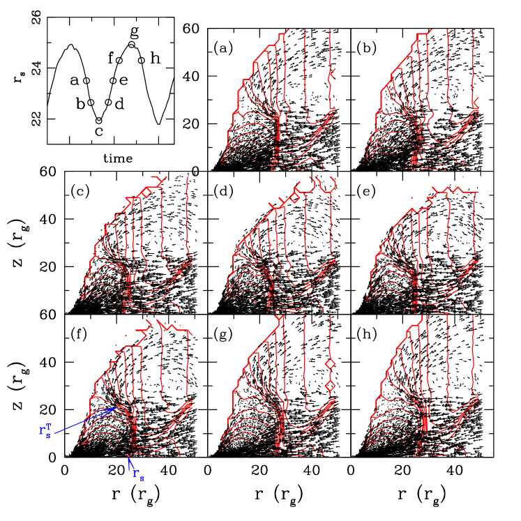
Figure 3: Velocity vectors are in the $r-z$ plane. SPH particles having angular momentum $\lambda_{inj}=1.63$ are injected supersonically from $r_{\rm inj}=50.4$ with injection velocity $v_{\rm inj}=-0.06436$ and sound speed $a_{inj}=0.06328$, respectively. Viscosity parameter is chosen as $\alpha=0.011$ and adiabatic index $\gamma=4/3$. Shock location oscillates with time. Figure 3(a-h) represent the various snap shots of velocity distribution taken at equal interval within a complete period of shock oscillation. In Figure 3f, $r^{T}_{s}$ and $r_{s}$ are indicated, and clearly there is a phase lag between the two. Here, Figure 3c denotes the case when shock location is closest from the black hole and Figure 3g represents the case when shock location is at its maximum value. Density contours (solid curves, red online) are plotted over the velocity vector field.

From Figs. 2c-2e, it is clear that the shock can experience persistent oscillation for some critical viscosity and injection parameters. But the shock front is a surface and that too not a rigid one. Therefore, every part of the shock front will not oscillate in the same phase, resulting in a phase lag between the shock front on and around the equatorial plane and the top of the shock front ($r^{T}_{s}$). For simplicity, we record the variation of shock location with time at the disc equatorial plane which is shown in top-left panel of Fig. 3. Note that there exists quasi-periodicity in the variation of shock location with time. We identify eight shock locations within a given oscillation period that are marked in open circles. The respective velocity field and density contours (solid, online red) of the flow in the $r-z$ plane is shown in the rest of the panels of Figs. 3(a-h). Higher density and extra thermal gradient force in the CENBOL region causes a fraction of in falling matter to bounce-off as outflow. When shock front oscillates, post-shock volume also oscillates which induces a periodic variation of driving force responsible to vertically remove a part of the in falling matter. As the shock reaches its minimum (Fig. 3c), the thermal driving of outflow is weak, so the spewed up matter falls back. The post-shock outflow continues to fall as the shock expands to its maxima (Figs. 3d, e, f). However, as the shock reaches its maximum value the thermal driving also recovers (Fig. 3g). The extra thermal driving plus the squeeze of the shock front as it shrinks, spews strong outflow (Fig. 3g). In Fig. 3f, we have indicated the shock location on the equatorial plane $r_{s}$, and the top of the shock front $r^{T}_{s}$. The position of the shock front can easily be identified from the clustering of the density contours connecting $r_{s}$ and $r^{T}_{s}$. From Figs. 3(a-h), it is clear that the mass outflow rate is significant when $r^{T}_{s}\lower 2.15277pt\hbox{$\;\buildrel>\over{\sim}\;$}r_{s}$.

Due to shock transition, the post shock matter becomes hot and dense which would essentially be responsible to emit high energy radiation. At the critical viscosity, since the shock front exhibits regular oscillation, the inner part of the disc, i.e., CENBOL, also oscillates indicating the variation of photon flux emanating from the disc. Thus, a correlation between the variation of shock front and emitted radiation seem to be viable. Usually, the bremsstrahlung emission is estimated as,

$$E_{Brem}=\int_{r_{1}}^{r_{2}}\rho^{2}T^{1/2}r^{2}dr,$$

where, $r_{1}$ and $r_{2}$ are the radii of interest within which radiation is being computed and $T$ is the local temperature. In this work, we calculate the total bremsstrahlung emission for the matter from the CENBOL region. Also, we quantify the mass outflow rate calculated assuming an annular cylinder at the injection radius which is concentric with the vertical axis. The thickness of the cylinder is considered to be twice the size of a SPH particle. This ensures at least one SPH particle lies within the cylindrical annulus. We identify particles leaving the computational domain as outflow provided they have positive resultant velocity, i.e., $v_{r}>0$ and $v_{z}>0$ and they lie above the disc height at the injection radius. With this, we estimate the mass outflow rate which is defined as $R_{\dot{m}}={\rm outflow~{}rate}~{}({\dot{M}}_{\rm out})/{\rm accretion~{}rate}~{}(|{\dot{M}}_{\rm in}|)$ and observe its time evolution. Here, ${\dot{M}}_{in(out)}=2\pi\rho_{\rm inj(out)}v_{\rm inj(out)}x_{\rm inj(out)}H_{\rm inj(out)}$. In Figure 4, we present the variation of shock location, corresponding bremsstrahlung flux from the post-shock region and mass outflow rate with time. Here, the radiative flux is plotted in arbitrary unit. Assuming a $10M_{\sun}$ black hole, the overall time evolution of five seconds ($\equiv$ 50600 code time) is shown for representation. The input parameters are $r_{\rm inj}=50.4$, $v_{\rm inj}=-0.06436$, $a_{\rm inj}=0.06328$, $\lambda_{\rm inj}=1.63$ and $\alpha=0.011$ respectively. Note that persistent shock oscillation takes place over a large time interval, with the oscillation amplitude $\sim 3r_{g}$. This phenomenon exhibits the emission of non-steady radiative flux which is nicely accounted as quasi-periodic variation commonly seen in many black hole candidates (Chakrabarti & Manickam, 2000; Remillard & McClintock, 2006). Subsequently, periodic mass ejection also results from the vicinity of the gravitating objects as a consequence of the modulation of the inner part of the disc due to shock oscillation.

To understand the correlation between the shock oscillation and the emitted photon flux from the inner part of the disc, we calculate the Fourier spectra of the quasi-periodic variation of the shock front and the power spectra of bremsstrahlung flux for matter resides within the boundary of post-shock region as well as outflow with resultant velocity $v>0$. The obtained results are shown in Figure 5, where the top panel is for shock oscillation, middle panel is for photon flux variation from post-shock disc and bottom panel is for photon flux variation of outflowing matter, respectively. Here, the input parameters are same as Figure 4. We find that the quasi-periodic variation of the shock location and the photon fluxes from post-shock disc and outflow are characterized by the fundamental frequency $\nu_{\rm fund}=3.7$ Hz which is followed by multiple harmonics. The first few prominent harmonic frequencies are $7.4$ Hz ($\sim 2\times\nu_{\rm fund}$), $11.2$ Hz ($\sim 3\times\nu_{\rm fund}$) and $14.2$ Hz ($\sim 4\times\nu_{\rm fund}$). This suggests that the dynamics of the inner part of the disc i.e., the post-shock disc and emitted fluxes are tightly coupled. In order to understand the generic nature of the above findings, we carried out another simulation with different input parameters. The results are shown in Figure 6, where we use $r_{\rm inj}=50.4~{}r_{g}$, $v_{\rm inj}=-0.06436$, $a_{\rm inj}=0.06328$, $\lambda_{\rm inj}=1.61$ and $\alpha=0.013$, respectively. The solutions are obtained similar to the previous case, i.e., first a steady state inviscid solution is obtained and then the viscosity is turned on. The corresponding Fourier spectra of shock oscillation and power spectra of radiative fluxes are presented in the top, middle and bottom panel, respectively. The obtained frequencies for quasi-periodic variations are $2.9~{}{\rm Hz}~{}{\rm\bf}~{}(\bf\nu_{\rm\bf fund})$, $5.6$ Hz ($\sim 2\times\nu_{\rm fund}$), $9.3$ Hz ($\sim 3\times\nu_{\rm fund}$) and $15$ Hz ($\sim 5\times\nu_{\rm fund}$). In both the cases, the obtained power density spectra (PDS) of emitted radiation has significant similarity with number of observational results (Remillard & McClintock, 2006; Nandi et al., 2012).

Figure 4: Top panel: Variation of shock location with time. Middle panel: Variation of the bremsstrahlung emission in arbitrary units with time. Bottom panel: Variation of mass outflow rate with time. Here, $\alpha=0.011$ and $M_{B}=10M_{\odot}$. Other parameters are same as Figure 3.

The quasi-periodicity that we observed in the power spectra of simulated results seems to be generic in nature. Several Galactic black hole sources exhibit QPO in the X-ray power spectra along with the harmonics. In Figure 7, we plotted one such observed X-ray power spectra of black hole source GX 339-4 of the 2010-11 outburst, which clearly shows the presence of fundamental QPO ($\sim$ 2.42 Hz) and harmonics at $\sim 4.88$ Hz and $\sim 7.20$ Hz (Nandi et al., 2012). This observational finding directly supports our simulation results and perhaps establishes the fact that the origin of such photon flux variation seems to be due to the hydrodynamic modulation of the inner part of the disc in terms of shock oscillation.

Recently, Nandi et al. (2013) reported the possible association of QPOs in X-rays and jets in the form of radio flares in outbursting black hole sources through the accretion flow dynamics. Here also we find that the dynamics of the post-shock disc region plays a major role for the jet generation and the emitted radiation. In other words, post-shock disc seems to be the precursor of jets as well as QPOs according to our present study.

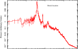
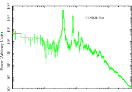
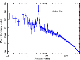
Figure 5: Top panel: Fourier spectra of shock location variation at the disc equatorial plane. Power spectra of bremsstrahlung flux variation calculated for SPH particles resides within the boundary of CENBOL (middle panel) and within the outflow region (bottom panel), respectively. Here, $\lambda_{\rm inj}=1.63$ and $\alpha=0.011$. In this case, we have consider simulated data of $\sim 20$ sec. Other parameters are same as Figure 1. Fundamental QPO frequency is obtained in both the cases $\sim 3.7$ Hz. However, significant differences in bremsstrahlung flux of CENBOL and outflow is observed.

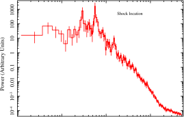
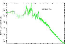
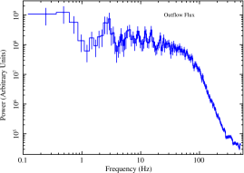
Figure 6: Top panel: Fourier spectra of shock location variation at the disc equatorial plane for $\lambda_{\rm inj}=1.61$ and $\alpha=0.013$. The other parameters are same as Figure 1. Power spectra of bremsstrahlung flux variation calculated for SPH particles resides within the boundary of CENBOL (middle panel) and within the outflow region (bottom panel), respectively. In this case, we have consider simulated data of $\sim 15$ sec. Fundamental QPO frequency is obtained in both the cases $\sim 2.9$ Hz.

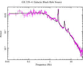
Figure 7: Signature of the multiple QPO frequencies ($\sim$2.42 Hz, 4.88 Hz & 7.20 Hz) observed in the power spectra of the galactic black hole source GX339-4.

4 Discussion and Concluding remarks

We have studied the dynamics of the viscous accretion flow around black holes using time dependent numerical simulation. While, accreting matter slows down against gravity as it experiences a barrier due to centrifugal force and eventually enter in to the black hole after triggering shock transition. Usually, post-shock flow is hot and compressed causing a thermal pressure gradient across the shock. As a result, it deflects part of the accreting matter as bipolar jet in a direction perpendicular to the disc equatorial plane. When viscosity is increased, shock becomes non-steady and ultimately starts oscillating when the viscosity reached its critical limit. Consequently, the outflowing matter also starts demonstrating quasi-periodic variation. Since the inner disc is hot and dense, high energy radiations must emit from the vicinity of the black holes. When the inner disc vibrates in radial direction, the emitted photon flux is also modulated. We compute the power density spectra of such behaviour and obtain fundamental peak at few Hz. We find that some of the harmonics are very prominent as seen in the observational results of several black hole candidates. The highlight of this paper is to show that the oscillation of shocked accretion flow shows QPOs with fundamentals as well as harmonics (Figs. 5, 6) as is seen from observations (Fig. 7). Interestingly, the bipolar outflow shows at least the fundamental frequency in its PDS for the case depicted in Figs. 5, however, the fundamental and harmonics are fairly weak in Figs. 6. So, this result suggests that photons from the outflows and jets would at least show the fundamental frequency, but probably no harmonics. Moreover, does this mean that if we happen to ‘see’ down the length of a jet, we would see quasi-periodic oscillations of photons in some jets (e.g., Figs. 5) and in some other jets the QPO signature would be washed out (e.g., Figs. 6)? And indeed in most blazars QPOs have not been detected, but in few QPO was found (Lachowicz et al., 2009). This issue need further investigation. Furthermore, while hot, dissipative flows show single shock, low energy dissipative flow showed multiple shocks (Lanzafame et al., 2008; Lee et al., 2011), however, the effect of high $\alpha$ has not been investigated.

The outflow also shows quasi-periodicity, however, blobs of matter are being ejected persistently with the oscillation of inner part of the disc, and therefore, such persistent activity will eventually give rise to a stream of matter and therefore a quasi-steady mildly relativistic jet. These ejections are not the ballistic relativistic ejections observed during the transition of hard-intermediate spectral state to the soft-intermediate spectral state. It has been recently shown that the momentum deposited by the disc photons on to jets, makes the jets stronger as the disc moves from LS to hard-intermediate spectral state (Kumar et al., 2014), simulations of which will be communicated elsewhere.

In this work, the mechanism studied for QPO generation is due to the perturbations induced by viscous dissipation and angular momentum transport. While it has been reported that QPOs can also be generated by cooling (Molteni et al., 1996b). In realistic disc, both processes are active, and both should produce shock oscillation. Interestingly though, viscosity can produce multiple shocks (for one spatial dimensional results see Lee et al. 2011), while no such thing has been reported with cooling processes, albeit investigations with cooling processes have not been done extensively. We would like to investigate the combined effect of cooling and viscous dissipation in future, to ascertain the viability of ‘shock cascade’ in much greater detail. It must be pointed out that this model of QPO and mass ejection (Nandi et al., 2001) can also be applied to the weakly magnetized accreting neutron stars. However, one has to change the inner boundary condition, i.e., put a hard surface as the inner boundary condition. The same methodology should also give rise to QPOs, and we are working on such a scenario, and would be reported elsewhere.

References

- Babul et al. (1989) Babul, A., Ostriker, J. P., Meszaros, P., ApJ, 1989, 347, 59
- Becker et al. (2008) Becker, P. A., Das, S., Le, T., 2008, ApJ, 677, L93
- Bondi (1952) Bondi, H., 1952, MNRAS, 112, 195
- Chakrabarti (1990) Chakrabarti, S. K., 1990, MNRAS, 243, 610.
- Chakrabarti & Titarchuk (1995) Chakrabarti, S. K., Titarchuk, L., 1995, ApJ, 455, 623
- Chakrabarti & Manickam (2000) Chakrabarti, S. K., Manickam, S. G., 2000, ApJL, 531, 41
- Chakrabarti & Das (2004) Chakrabarti, S. K., Das, S., 2004, MNRAS, 349, 649
- Chakrabarti et al. (2008) Chakrabarti, S. K., Debnath, D., Nandi, A., Pal, P. S., 2008, A&A, 489, L41
- Chang & Ostriker (1985) Chang, K. M., Ostriker, J. P., 1985, ApJ, 288, 428
- Chattopadhyay (2008) Chattopadhyay, I., 2008, in Chakrabarti S. K., Majumdar A. S., eds, AIP Conf. Ser. Vol. 1053, Proc. 2nd Kolkata Conf. on Observational Evidence of Back Holes in the Universe and the Satellite Meeting on Black Holes Neutron Stars and Gamma-Ray Bursts. Am. Inst. Phys., New York, p. 353
- Chattopadhyay & Das (2007) Chattopadhyay, I., Das, S., 2007, New A, 12, 454
- Chattopadhyay & Chakrabarti (2011) Chattopadhyay I., Chakrabarti S.K., 2011, Int. Journ. Mod. Phys. D, 20, 1597
- Chattopadhyay & Kumar (2013) Chattopadhyay, I., Kumar, R., 2013, ASI Conf. Ser., 8, 19
- Das et al. (2001) Das, S., Chattopadhyay, I., Nandi, A., Chakrabarti, S. K., 2001, A&A, 379, 683
- Das (2007) Das, S., 2007, MNRAS, 376, 1659
- Das & Chattopadhyay (2008) Das, S., Chattopadhyay I., 2008, New A, 13, 549
- Das et al. (2009) Das, S.; Becker, P. A.; Le, T., 2009, ApJ, 702, 649
- Doeleman et al. (2012) Doeleman, S., S., et al. 2012, Science, 338, 355
- Fukue (1987) Fukue, J., 1987, PASJ, 39, 309
- Fukumura & Kazanas (2007) Fukumura, K., Kazanas, D., 2007, ApJ, 669, 85
- Gallo et al. (2003) Gallo, E., Fender, R. P., Pooley, G. G. 2003, MNRAS, 344, 60
- Junor et al. (1999) Junor, W., Biretta, J. A., Livio, M., 1999, Nature, 401, 891
- Kazanas & Ellison (1986) Kazanus, D., Ellison, D. C., 1986, ApJ, 304, 178
- Kumar & Chattopadhyay (2013) Kumar R., Chattopadhyay I., 2013, MNRAS, 430, 386
- Kumar et al. (2013) Kumar, R., Singh, C. B., Chattopadhyay, I., Chakrabarti, S. K., 2013, MNRAS, 436, 2864
- Kumar et al. (2014) Kumar, R., Chattopadhyay, I., Mandal, S., 2014, MNRAS, 437, 2992
- Lachowicz et al. (2009) Lachowicz, P., Gupta, A. C., Gaur, H., Wiita, P. J., 2009, A&A, 506, L 17
- Lanzafame et al. (1998) Lanzafame, G., Molteni, D., Chakrabarti, S. K., 1998, MNRAS, 299, 799
- Lanzafame et al. (2008) Lanzafame, G., Cassaro, P., Schilliró, F., Costa, V., Belvedere, G., Zapalla, R. A., 2008, A&A, 473, 482
- Le & Becker (2005) Le, T., Becker, P. A., 2005, ApJ, 632, 476
- Lee et al. (2011) Lee, S. J., Ryu, D., Chattopadhyay, I., 2011, ApJ, 728, 142
- Liang & Thompson (1980) Liang, E. P. T., Thompson, K. A., 1980, ApJ, 240, 271
- Livio (1999) Livio, M., 1999, Phys. Rep., 311, 225
- Lu et al. (1999) Lu, J. F., Gu, W. M., Yuan, F., 1999, ApJ, 523, 340
- Mandal & Chakrabarti (2010) Mandal, S., Chakrabarti, S. K., 2010, ApJ, 710, L 147
- McHardy et al. (2006) McHardy, I. M., Koerding, E., Knigge, C., Fender, R. P., 2006, Nature, 444, 730
- Michel (1972) Michel, F. C., 1972, Ap&SS, 15, 153
- Miller-Jones et al. (2012) Miller-Jones, C. J. A., et al. , 2012, MNRAS, 421, 468
- Molteni et al. (1994) Molteni, D., Lanzafame, G., Chakrabarti, S. K., 1994, ApJ, 425, 161
- Molteni et al. (1996a) Molteni, D., Ryu, D., Chakrabarti, S. K., 1996a, ApJ, 470, 460
- Molteni et al. (1996b) Molteni, D., Sponholtz, H., Chakrabarti, S. K., 1996b, ApJ, 457, 405
- Molteni et al. (2006) Molteni, D., Gerardi, G., Teresi, V., 2006, MNRAS, 365, 1405
- Monaghan (1992) Monaghan, J. J., 1992, ARA&A, 30, 543
- Narayan et al. (1997) Narayan, R., Kato, S., Honma, F., 1997, ApJ, 476, 49
- Nandi et al. (2001) Nandi, A., Chakrabarti, S. K., Vadawale, S. V., Rao, A. R., 2001, A&A, 380, 245
- Nandi et al. (2012) Nandi, A., Debnath, D., Mandal, S., Chakrabarti, S. K., 2012, A&A, 542, 56
- Nandi et al. (2013) Nandi, A., Radhika, D. A., Seetha, S., 2013, ASI Conf. Ser., 8, 71
- Paczyński & Wiita (1980) Paczyński, B., Wiita, P., 1980, A&A, 88, 23
- Radhika & Nandi (2013) Radhika, D. A., Nandi, A., 2013, arXiv1308.3138
- Remillard & McClintock (2006) Remillard, R. A., McClintock, J. E., 2006, ARA&A, 44, 49
- Rushton et al. (2010) Rushton, A., Spencer R., Fender, R., Pooley, G., 2010, A&A, 524, 29
- Shakura & Sunyaev (1973) Shakura, N. I.; Sunyaev, R. A., 1973, A&A, 24, 337
- Shapiro (1973) Shapiro, S., 1973, ApJ, 180, 531
- Shaposhnikov & Titarchuk (2009) Shaposhnikov, N., Titarchuk, L., 2009, ApJ, 699, 453