A Nonlinear Multigrid Steady-State Solver for Microflow

Abstract

We develop a nonlinear multigrid method to solve the steady state of microflow, which is modeled by the high order moment system derived recently for the steady-state Boltzmann equation with ES-BGK collision term. The solver adopts a symmetric Gauss-Seidel iterative scheme nested by a local Newton iteration on grid cell level as its smoother. Numerical examples show that the solver is insensitive to the parameters in the implementation thus is quite robust. It is demonstrated that expected efficiency improvement is achieved by the proposed method in comparison with the direct time-stepping scheme.

Keywords: Multigrid; Boltzmann equation; ES-BGK model; NR$xx$ method

1 Introduction

The Boltzmann equation plays an important role in various fields of modern kinetic theory, e.g., rarefied gas flows, microflows and semiconductor device simulations. Due to its high dimension of variables, numerical simulation of these problems is extremely expensive, even though its complicated collision operator (see e.g. [13]) is replaced by other simplified collision operators, such as the Bhatnagar-Gross-Krook (BGK) model [1], the ellipsoidal statistical BGK (ES-BGK) model [17], the Shakhov model [29], the Maxwell molecules model [14], etc. Lots of work has been done to reduce the computational costs in numerical solution of the Boltzmann equation or its simplified collision models over the past few decades. The moment method, originally introduced by Grad [15], was considered as one of the candidates in this direction.

The objective of the moment method is to approximate the Boltzmann equation using a small number of variables. Based on the Hermite expansion in the velocity space of the distribution function, moment equations were derived from the Boltzmann equation. These equations can be viewed as extended hydrodynamic-like equations in a macroscopic point of view. In terms of numerical method, they are actually a semi-discretization of the Boltzmann equation, where the velocity space is discretized by the Hermite spectral method. Moreover, these equations are highly nonlinear and coupled with each other, as the classical Euler equations. Meanwhile, the lack of global hyperbolicity of Grad’s original moment system [28, 12] restricts its application during a long time. Recently, with a certain regularization, a systematic numerical method, abbreviated as the NR$xx$ method, has been developed in [6, 10, 9, 7] to solve the moment system derived for the Boltzmann equation. The unified framework of the NR$xx$ method makes it is easy to implement the system with moments up to arbitrary order. In [3] and [4], a new regularization without any additionally empirical parameters was proposed such that the resulting moment system is globally hyperbolic, which is essential in the local well-posedness of the system.

While the NR$xx$ method has been found to be effective for various problems, see e.g. [11, 5, 8, 20], the state-of-the-art numerical techniques to improve its efficiency have not been sufficiently explored, especially for the steady-state problems. On the other hand, there are quite some important applications for the Boltzmann equation, where the main concern is the steady-state solution. For steady-state problems, some additional acceleration techniques, including implicit time-stepping schemes [26, 27], various iterative methods [22], multigrid accelerations [2, 16], which are originally developed for classical hydrodynamics [21, 18, 19, 23, 24], may be employed to further improve the numerical efficiency. Aiming on improving the efficiency of the steady-state solver following these methods, we are mainly concerned in this paper with the development of multigrid solution strategy for the moment system derived for the steady-state Boltzmann equation.

The basic procedure of our current exploration is as below. At first, we discretize the target moment system under the unified framework of the NR$xx$ method as in [6], so that the multigrid solver we develop is also unified for the system with moments up to arbitrary order. We then present a nonlinear iterative method on a single grid level to solve the resulting discretized system, which is a set of nonlinear coupled equations as mentioned in the following sections. This nonlinear iteration is formulated as a nested iterative scheme which is combined by an inner iteration and an outer iteration. We take a cell by cell symmetric Gauss-Seidel (SGS) iteration as the outer iteration to reduce the global nonlinear system into a local nonlinear system with respect to the local variables on each cell. For the inner iteration, the Newton type method is employed to solve the local nonlinear system on each cell. Due to the nonlinear coupling of the variables in the system, it is quite difficult to derive the analytical expression of the local Jacobian matrix. As an alternative, we calculate the local Jacobian matrix through the numerical differentiation and regularize it by the local residual as in [21]. The relaxation parameter, in the step of updating solution of the Newton iteration, is computed adaptively to preserve positive density and temperature. It is verified by numerical examples that our method converges much faster than the direct time-stepping NR$xx$ scheme.

The nonlinear iteration is taken as smoother in a multigrid framework for further acceleration. The multigrid method we adopt is the nonlinear multigrid (NMG) algorithm developed in [16]. The NMG algorithm therein is quite formal, therefore we only need a strategy to generate a sequence of coarse grids from the finest grid, and operators to transfer the solution between two successive grids. For the moment system under our current consideration, which is 1D in spatial coordinates, the coarse grid can be generated directly by an intuitive way, namely, a coarse grid cell consists of two adjacent fine grid cells. After the coarse grids have been obtained, the restriction operator, to transfer the fine grid solution onto the coarse grid, is then constructed locally. Precisely, the coarse grid solution on a coarse grid cell is only determined by the fine grid solution on the corresponding fine grid cells. For the prolongation operator from the coarse grid to the fine grid, the identical operator is simply utilized.

The rest part of this paper is organized as follows. In section 2, we give a brief review of the steady-state Boltzmann equation with ES-BGK collision term and its hyperbolic moment system, followed with the unified discretization. We then present in section 3 the details of the basic nonlinear iterative method on a single grid level. In section 4, the nonlinear multigrid solver using the basic iteration as smoother is introduced. Two numerical examples are carried out in section 5 to demonstrate the robustness and efficiency of the proposed multigrid solver. Some concluding remarks are given in the last section.

2 Moment System of Boltzmann Equation

The Boltzmann equation in steady state can be written as

$$\boldsymbol{\xi}\cdot\nabla_{\boldsymbol{x}}f+\boldsymbol{F}\cdot\nabla_{\boldsymbol{\xi}}f=Q(f),$$ (1)

where $f(\boldsymbol{x},\boldsymbol{\xi})$ is the particle distribution function of position $\boldsymbol{x}\in\Omega\subset\mathbb{R}^{D}$ $(D=1,2,\text{or }3)$ and molecular velocity $\boldsymbol{\xi}\in\mathbb{R}^{3}$. The vector $\boldsymbol{F}$ is the external force accelerating particles, and the right hand side $Q(f)$ is the collision term modeling the interaction between particles. Since the original Boltzmann collision term contains a five-dimensional integral (see e.g. [13] for the detailed form), it turns out to be too complicated to handle for numerical solution. Therefore, a variety of simplified collision models were raised to approximate it. In this paper, we take the ES-BGK model as an example to present our method.

The ES-BGK collision term reads

$$Q(f)=\nu(f^{\text{ES}}-f),$$ (2)

where $\nu$ is the average collision frequency given by

$$\nu=\Pr\frac{\rho\theta}{\mu},$$ (3)

and $f^{\text{ES}}$ is an anisotropic Gaussian distribution with the form as

$$f^{\text{ES}}(\boldsymbol{x},\boldsymbol{\xi})=\frac{\rho(\boldsymbol{x})}{m\sqrt{\det[2\pi{\boldsymbol{\Lambda}}(\boldsymbol{x})]}}\exp\left(-\frac{1}{2}(\boldsymbol{\xi}-\boldsymbol{u}(\boldsymbol{x}))^{T}[{\boldsymbol{\Lambda}}(\boldsymbol{x})]^{-1}(\boldsymbol{\xi}-\boldsymbol{u}(\boldsymbol{x}))\right),$$ (4)

in which ${\boldsymbol{\Lambda}}=(\lambda_{ij})$ is a $3\times 3$ matrix with

$$\lambda_{ij}(\boldsymbol{x})=\theta(\boldsymbol{x})\delta_{ij}+\left(1-\frac{1}{\Pr}\right)\frac{\sigma_{ij}(\boldsymbol{x})}{\rho(\boldsymbol{x})},\quad i,j=1,2,3.$$ (5)

Here, $\Pr$ is the Prandtl number, $\mu$ is the viscosity, and $m$ is the mass of a single particle. The macroscopic quantities, including density $\rho$, velocity $\boldsymbol{u}$, temperature $\theta$, and stress tensor $\sigma_{ij}$, are related with $f$ by

$$\begin{aligned} &\rho(\boldsymbol{x})=m\int_{\mathbb{R}^{3}}f(\boldsymbol{x},\boldsymbol{\xi})\,\mathrm{d}\boldsymbol{\xi},\quad\rho(\boldsymbol{x})\boldsymbol{u}(\boldsymbol{x})=m\int_{\mathbb{R}^{3}}\boldsymbol{\xi}f(\boldsymbol{x},\boldsymbol{\xi})\,\mathrm{d}\boldsymbol{\xi},\\ &\rho(\boldsymbol{x})|\boldsymbol{u}(\boldsymbol{x})|^{2}+3\rho(\boldsymbol{x})\theta(\boldsymbol{x})=m\int_{\mathbb{R}^{3}}|\boldsymbol{\xi}|^{2}f(\boldsymbol{x},\boldsymbol{\xi})\,\mathrm{d}\boldsymbol{\xi},\\ &\sigma_{ij}(\boldsymbol{x})=m\int_{\mathbb{R}^{3}}(\xi_{i}-u_{i}(\boldsymbol{x}))(\xi_{j}-u_{j}(\boldsymbol{x}))f(\boldsymbol{x},\boldsymbol{\xi})\,\mathrm{d}\boldsymbol{\xi}-\rho(\boldsymbol{x})\theta(\boldsymbol{x})\delta_{ij},\quad i,j=1,2,3.\end{aligned}$$ (6)

Additionally, the heat flux $\boldsymbol{q}$ is defined by

$$\boldsymbol{q}(\boldsymbol{x})=\frac{m}{2}\int_{\mathbb{R}^{3}}|\boldsymbol{\xi}-\boldsymbol{u}(\boldsymbol{x})|^{2}(\boldsymbol{\xi}-\boldsymbol{u}(\boldsymbol{x}))f(\boldsymbol{x},\boldsymbol{\xi})\,\mathrm{d}\boldsymbol{\xi}.$$ (7)

In [8], a hyperbolic moment system was derived for the time-dependent Boltzmann equation with the ES-BGK collision term and without the external force term (see [7] for the treatment of the force term). By setting the time derivatives to 0 in that system, we can obtain a steady-state counterpart for equation (1). Nevertheless, we briefly review the derivation of the steady-state moment system below.

The starting point is the approximation of $f$ by an $M$-th order truncated series as

$$f(\boldsymbol{x},\boldsymbol{\xi})\approx\sum_{|\alpha|\leq M}f_{\alpha}(\boldsymbol{x})\mathcal{H}_{\theta(\boldsymbol{x}),\alpha}\left(\frac{\boldsymbol{\xi}-\boldsymbol{u}(\boldsymbol{x})}{\sqrt{\theta(\boldsymbol{x})}}\right),$$ (8)

where $M>2$ is a positive integer, $\alpha=(\alpha_{1},\alpha_{2},\alpha_{3})\in\mathbb{N}^{3}$ is a three-dimensional multi-index and $|\alpha|=\alpha_{1}+\alpha_{2}+\alpha_{3}$. The basis functions $\mathcal{H}_{\theta,\alpha}$ are defined by

$$\mathcal{H}_{\theta,\alpha}(\boldsymbol{v})=\frac{1}{m(2\pi\theta)^{3/2}\theta^{|\alpha|/2}}\prod\limits_{d=1}^{3}\mathit{He}_{\alpha_{d}}(v_{d})\exp\left(-\frac{v_{d}^{2}}{2}\right),\quad\forall\alpha\in\mathbb{N}^{3},~{}\boldsymbol{v}\in\mathbb{R}^{3},$$ (9)

where $\mathit{He}_{n}(x)$ is the Hermite polynomial of order $n$ as

$$\mathit{He}_{n}(x)=(-1)^{n}\exp\left(\frac{x^{2}}{2}\right)\frac{\,\mathrm{d}^{n}}{\,\mathrm{d}x^{n}}\exp\left(-\frac{x^{2}}{2}\right).$$ (10)

With the help of the orthogonality of Hermite polynomials, the expansion (8) together with (6) and (7) yields

$$\begin{aligned} &f_{0}=\rho,\qquad f_{e_{1}}=f_{e_{2}}=f_{e_{3}}=0,\qquad\sum_{d=1}^{3}f_{2e_{d}}=0,\\ &\sigma_{ij}=(1+\delta_{ij})f_{e_{i}+e_{j}},\quad q_{i}=2f_{3e_{i}}+\sum_{d=1}^{3}f_{2e_{d}+e_{i}},\qquad i,j=1,2,3,\end{aligned}$$ (11)

where $\delta_{ij}$ is the Kronecker delta symbol, and $e_{1}$, $e_{2}$, $e_{3}$ are introduced to denote the multi-indices $(1,0,0)$, $(0,1,0)$, $(0,0,1)$, respectively.

Substituting the expansion (8) into the Boltzmann equation (1), matching the coefficients of the same basis function, and regularizing it by the regularization proposed in [4], we obtain the final moment system as follows

$$\begin{split}&\sum_{j=1}^{D}\Bigg{[}\left(\theta\frac{\partial f_{\alpha-e_{j}}}{\partial x_{j}}+u_{j}\frac{\partial f_{\alpha}}{\partial x_{j}}+(1-\delta_{|\alpha|,M})(\alpha_{j}+1)\frac{\partial f_{\alpha+e_{j}}}{\partial x_{j}}\right)\\ &+\sum_{d=1}^{3}\frac{\partial u_{d}}{\partial x_{j}}\left(\theta f_{\alpha-e_{d}-e_{j}}+u_{j}f_{\alpha-e_{d}}+(1-\delta_{|\alpha|,M})(\alpha_{j}+1)f_{\alpha-e_{d}+e_{j}}\right)\\ &+\frac{1}{2}\frac{\partial\theta}{\partial x_{j}}\sum_{d=1}^{3}\left(\theta f_{\alpha-2e_{d}-e_{j}}+u_{j}f_{\alpha-2e_{d}}+(1-\delta_{|\alpha|,M})(\alpha_{j}+1)f_{\alpha-2e_{d}+e_{j}}\right)\Bigg{]}\\ &=\sum_{d=1}^{3}F_{d}f_{\alpha-e_{d}}+\nu(f^{\text{ES}}_{\alpha}-f_{\alpha}),\qquad|\alpha|\leq M,\end{split}$$ (12)

where $f^{\text{ES}}_{\alpha}$ are coefficients of the expansion of the Gaussian distribution $f^{\text{ES}}$, namely,

$$f^{\text{ES}}(\boldsymbol{x},\boldsymbol{\xi})=\sum_{|\alpha|\leq M}f^{\text{ES}}_{\alpha}(\boldsymbol{x})\mathcal{H}_{\theta(\boldsymbol{x}),\alpha}\left(\frac{\boldsymbol{\xi}-\boldsymbol{u}(\boldsymbol{x})}{\sqrt{\theta(\boldsymbol{x})}}\right).$$ (13)

It follows from [8] that $f^{\text{ES}}_{\alpha}$ can be calculated recursively by

$$f^{\text{ES}}_{\alpha}=\left\{\begin{aligned} &\rho,&&\text{if}~{}\alpha=0,\\ &0,&&\text{if}~{}|\alpha|=1,\\ &\frac{1-1/\Pr}{\alpha_{i}\rho}\sum_{j=1}^{3}\sigma_{ij}f^{\text{ES}}_{\alpha-e_{i}-e_{j}},&&{\text{if}}~{}|\alpha|\geq 2~{}{\text{and}}~{}\alpha_{i}>0.\end{aligned}\right.$$ (14)

At first glance, it is sufficient to note that the moment system (12) is a set of nonlinear coupled equations for the moments $\boldsymbol{u},\theta,f_{\alpha}$.

For practical applications, the moment system (12) has to be equipped with proper boundary conditions. In kinetic theory, the Maxwell boundary condition proposed in [25] is frequently used. The version of the Maxwell boundary condition for moment system was derived in [7] and demonstrated its well-posedness for the hyperbolic moment system in [8]. Accordingly, we adopt these boundary conditions in this paper. We refer to [7, 8] for details on these boundary conditions.

Since we are focusing on the iterative method to the steady-state problem, we discretize the steady-state moment system following the method in [6, 8]. The distribution function (8) is the unknown in the discretized problem, which is constructed by $\boldsymbol{u},\theta$ and $f_{\alpha}$. For simplicity of notations, we introduce $\mathcal{F}_{M}(\boldsymbol{u},\theta)$ to denote the linear space spanned by $\mathcal{H}_{\theta,\alpha}\left(\frac{\boldsymbol{\xi}-\boldsymbol{u}}{\sqrt{\theta}}\right)$, $|\alpha|\leq M$. It follows that $\mathcal{F}_{M}(\boldsymbol{u},\theta)$ forms a finite dimensional subspace of $L^{2}\left(\mathbb{R}^{3},\exp\left(|\boldsymbol{\xi}-\boldsymbol{u}|^{2}/(2\theta)\right)\,\mathrm{d}\boldsymbol{\xi}\right)$. In our numerical scheme, it is also allowed to approximate the distribution function $f$ in another linear space $\mathcal{F}_{M}(\boldsymbol{u}^{\prime},\theta^{\prime})$ with the relation (11) violated. However, if it is not pointed out, $f$ always belongs to the space where (11) holds, i.e., the parameters of the space, $\boldsymbol{u}$ and $\theta$, are macroscopic velocity and temperature of $f$ respectively. A fast transformation between two spaces, $\mathcal{F}_{M}(\boldsymbol{u},\theta)$ and $\mathcal{F}_{M}(\boldsymbol{u}^{\prime},\theta^{\prime})$, can be found in [6].

We restrict ourselves to one spatial dimensional case in the following. Suppose the spatial domain, which is an interval $[a,b]$, is divided by the mesh

$$a=x_{0}<x_{1}<\cdots<x_{N-1}<x_{N}=b,$$

and let $\Delta x_{i}=x_{i+1}-x_{i}$. Then the finite volume discretization for the steady-state moment system (12) over the $i$-th cell $[x_{i},x_{i+1}]$ is given by

$$\frac{F(f_{i}(\boldsymbol{\xi}),f_{i+1}(\boldsymbol{\xi}))-F(f_{i-1}(\boldsymbol{\xi}),f_{i}(\boldsymbol{\xi}))}{\Delta x_{i}}=G(f_{i}(\boldsymbol{\xi}))+Q(f_{i}(\boldsymbol{\xi})),$$ (15)

where $f_{i}(\boldsymbol{\xi})\in\mathcal{F}_{M}(\boldsymbol{u}_{i},\theta_{i})$ is the approximation of the distribution function on the $i$-th cell. Note that the distribution function on the ghost cells, $f_{-1}(\boldsymbol{\xi})$ and $f_{N}(\boldsymbol{\xi})$, are dependent on $f_{0}(\boldsymbol{\xi})$ and $f_{N-1}(\boldsymbol{\xi})$, respectively, for the Maxwell boundary condition.

The numerical flux $F(f_{i},f_{i+1})$ is defined on $x_{i+1}$, the boundary between the $i$-th and $(i+1)$-th cells. To compare the solution with [8], the same numerical flux, a non-conservative version of the HLL flux, is considered. We omit its expression here, since it is enough to know that the numerical fluxes, $F(f_{i-1},f_{i})$ and $F(f_{i},f_{i+1})$ of (15), are approximated in $\mathcal{F}_{M}(\boldsymbol{u}_{i},\theta_{i})$, i.e.,

$$\begin{aligned} &F(f_{i-1},f_{i})=\sum_{|\alpha|\leq M}F_{\alpha}(f_{i-1},f_{i})\mathcal{H}_{\theta_{i},\alpha}\left(\frac{\boldsymbol{\xi}-\boldsymbol{u}_{i}}{\sqrt{\theta_{i}}}\right),\\ &F(f_{i},f_{i+1})=\sum_{|\alpha|\leq M}F_{\alpha}(f_{i},f_{i+1})\mathcal{H}_{\theta_{i},\alpha}\left(\frac{\boldsymbol{\xi}-\boldsymbol{u}_{i}}{\sqrt{\theta_{i}}}\right),\end{aligned}$$ (16)

and the computation of these numerical fluxes requires the fast transformation between $\mathcal{F}_{M}(\boldsymbol{u}_{i},\theta_{i})$ and $\mathcal{F}_{M}(\boldsymbol{u}_{i\pm 1},\theta_{i\pm 1})$.

Similarly to the numerical flux, the external force term $G(f_{i})$ and the collision term $Q(f_{i})$, are also approximated in $\mathcal{F}_{M}(\boldsymbol{u}_{i},\theta_{i})$, i.e.,

$$G(f_{i}(\boldsymbol{\xi}))=\sum_{|\alpha|\leq M}G_{i,\alpha}\mathcal{H}_{\theta_{i},\alpha}\left(\frac{\boldsymbol{\xi}-\boldsymbol{u}_{i}}{\sqrt{\theta_{i}}}\right),$$ (17)

$$Q(f_{i}(\boldsymbol{\xi}))=\sum_{|\alpha|\leq M}Q_{i,\alpha}\mathcal{H}_{\theta_{i},\alpha}\left(\frac{\boldsymbol{\xi}-\boldsymbol{u}_{i}}{\sqrt{\theta_{i}}}\right),$$ (18)

where $G_{i,\alpha}=\sum_{d=1}^{3}F_{d}f_{i,\alpha-e_{d}}$ and $Q_{i,\alpha}=\nu(f_{i,\alpha}^{\text{ES}}-f_{i,\alpha})$.

3 Single Grid Solver

Define the local residual on the $i$-th cell as

$$R_{i}(f_{i-1},f_{i},f_{i+1})=\frac{F(f_{i}(\boldsymbol{\xi}),f_{i+1}(\boldsymbol{\xi}))-F(f_{i-1}(\boldsymbol{\xi}),f_{i}(\boldsymbol{\xi}))}{\Delta x_{i}}-G(f_{i}(\boldsymbol{\xi}))-Q(f_{i}(\boldsymbol{\xi})).$$ (19)

Then the discretization (15) is re-written as

$$R_{i}(f_{i-1},f_{i},f_{i+1})=r_{i}(\boldsymbol{\xi}),$$ (20)

where $r_{i}(\boldsymbol{\xi})$ is independent of $f$ and is introduced to give a slightly more general problem. For (15), we have $r_{i}(\boldsymbol{\xi})\equiv 0$. It is clear that the problem (20) is nonlinear and we prefer a nested iterative strategy, which uses a cell by cell SGS iteration as the outer iteration, and a local Newton iteration as the inner iteration.

Given an approximate solution $f_{i}^{n}(\boldsymbol{\xi})$, $i=0,1,\ldots,N-1$, the new approximate solution $f_{i}^{n+1}(\boldsymbol{\xi})$ of an SGS iterative step is formulated into two loops as

1. Loop $i$ increasingly from 0 to $N-1$, obtain $f_{i}^{n+\frac{1}{2}}(\boldsymbol{\xi})$ by solving

   $$R_{i}(f_{i-1}^{n+\frac{1}{2}},f_{i}^{n+\frac{1}{2}},f_{i+1}^{n})=r_{i}(\boldsymbol{\xi}).$$ (21)

2. Loop $i$ decreasingly from $N-1$ to $0$, obtain $f_{i}^{n+1}(\boldsymbol{\xi})$ by solving

   $$R_{i}(f_{i-1}^{n+\frac{1}{2}},f_{i}^{n+1},f_{i+1}^{n+1})=r_{i}(\boldsymbol{\xi}).$$ (22)

Both (21) and (22) are local nonlinear problems with the distribution function $f_{i}(\boldsymbol{\xi})$ as the only unknown, and thereby are solved by the Newton method. Removing the superscripts and the dependence on $f_{i-1}(\boldsymbol{\xi})$, $f_{i+1}(\boldsymbol{\xi})$, these problems are abbreviated to the following form

$$R_{i}(f_{i})=r_{i}(\boldsymbol{\xi}).$$ (23)

Now let $f_{i}^{(m)}(\boldsymbol{\xi})$ is an approximation of $f_{i}(\boldsymbol{\xi})$ and re-expand $f_{i}(\boldsymbol{\xi})$ in $\mathcal{F}_{M}(\boldsymbol{u}_{i}^{(m)},\theta_{i}^{(m)})$, that is,

$$f_{i}(\boldsymbol{\xi})=\sum_{|\alpha|\leq M}f_{i,\alpha}\mathcal{H}_{\theta_{i}^{(m)},\alpha}\left(\frac{\boldsymbol{\xi}-\boldsymbol{u}_{i}^{(m)}}{\sqrt{\theta_{i}^{(m)}}}\right).$$ (24)

It is trivial to see that $f_{i}(\boldsymbol{\xi})$ is determined by the coefficients $f_{i,\alpha}$ of (24), which follows that the local residual $R_{i}(f_{i})$ is also determined by $f_{i,\alpha}$. Consequently, the linearization of (23) by the Newton method is given as

$$\begin{aligned} \sum_{|k|\leq M}\frac{\delta R_{i}(f_{i}^{(m)})}{\delta f_{i,k}}\Delta f_{i,k}^{(m)}=\tilde{R}_{i}^{(m)}=r_{i}(\boldsymbol{\xi})-R_{i}(f_{i}^{(m)}),\end{aligned}$$ (25)

where the formal derivatives $\delta R_{i}/\delta f_{i,k}$ are calculated by the numerical differentiation method as

$$\frac{\delta R_{i}(f_{i}^{(m)})}{\delta f_{i,k}}=\frac{R_{i}(\tilde{f}_{i}^{(m),k})-R_{i}(f_{i}^{(m)})}{\delta f_{i,k}},$$ (26)

where

$$\tilde{f}_{i}^{(m),k}(\boldsymbol{\xi})=f_{i}^{(m)}(\boldsymbol{\xi})+\delta f_{i,k}\mathcal{H}_{\theta_{i}^{(m)},k}\left(\frac{\boldsymbol{\xi}-\boldsymbol{u}_{i}^{(m)}}{\sqrt{\theta_{i}^{(m)}}}\right),$$

and $\delta f_{i,k}$ is a small perturbation of the coefficients. As mentioned in previous section, the residual $R_{i}(f_{i})$, as well as $r_{i}(\boldsymbol{\xi})$ and its formal derivatives $\delta R_{i}/\delta f_{i,k}$, is calculated to a result in $\mathcal{F}_{M}(\boldsymbol{u}_{i}^{(m)},\theta_{i}^{(m)})$. Let the corresponding coefficients be $R_{i,\alpha}(f_{i})$, $r_{i,\alpha}$ and $J_{i,\alpha,k}$, respectively. Then by matching the coefficients of the same basis function, we can deduce an equivalent linear system for (25) as

$$\boldsymbol{J}\Delta\boldsymbol{f}_{i}^{(m)}=\tilde{\boldsymbol{R}}_{i}^{(m)},$$ (27)

where $\boldsymbol{J}=(J_{i,\alpha,k})$ is the Jacobian matrix, and $\Delta\boldsymbol{f}_{i}^{(m)}$, $\tilde{\boldsymbol{R}}_{i}^{(m)}$ are the vectors of $\Delta f_{i,\alpha}^{(m)}$, $\tilde{R}_{i,\alpha}^{(m)}=r_{i,\alpha}-R_{i,\alpha}(f_{i}^{(m)})$, respectively.

Since the linear problem (27) might be singular, to make the iteration stable while keeping the convergence speed, it is regularized by the local residual as in [21], which yields

$$\begin{aligned} \left(\lambda\left\|\tilde{R}_{i}^{(m)}\right\|\boldsymbol{I}+\boldsymbol{J}\right)\Delta\boldsymbol{f}_{i}^{(m)}=\tilde{\boldsymbol{R}}_{i}^{(m)},\end{aligned}$$ (28)

where $\boldsymbol{I}$ is the identity matrix, $\lambda$ is a parameter, and $\left\|\tilde{R}_{i}^{(m)}\right\|$ is a norm of the residual $\tilde{R}_{i}^{(m)}$. In our numerical examples, $\lambda$ is insensitive and is often set as 1. The $L^{2}$ norm, equipped for the linear space $\mathcal{F}_{M}(\boldsymbol{u}_{i}^{(m)},\theta_{i}^{(m)})$, is employed for $\|\cdot\|$, which is turned out to be

$$\left\|\tilde{R}_{i}^{(m)}\right\|=\sqrt{\sum_{|\alpha|\leq M}C_{\alpha}\left|\tilde{R}_{i,\alpha}^{(m)}\right|^{2}},$$ (29)

where $C_{\alpha}=(2\pi)^{-3/2}\left(\theta_{i}^{(m)}\right)^{-|\alpha|-3}\alpha!$ and $\alpha!=\alpha_{1}!\alpha_{2}!\alpha_{3}!$.

While obtaining $\Delta\boldsymbol{f}_{i}^{(m)}$ from (28), the solution is then updated by

$$f_{i,\alpha}^{*}=f_{i,\alpha}^{(m)}+\tau\Delta f_{i,\alpha}^{(m)},$$ (30)

where $\tau$ is a relaxation parameter set as $\tau=\min\{1,\hat{\tau}\}$, in which $\hat{\tau}>0$ is a parameter to preserve the positivity of the local density and temperature. The computation of $\hat{\tau}$ is not difficult but tedious, hence we present it in Appendix A.

The updated approximation $f_{i}^{*}(\boldsymbol{\xi})$, obtained until now, belongs to $\mathcal{F}_{M}(\boldsymbol{u}_{i}^{(m)},\theta_{i}^{(m)})$ and usually does not satisfy the relation (11). An additional step is utilized such that the expansion of the new approximation satisfies (11). To this end, compute the new macroscopic velocity $\boldsymbol{u}_{i}^{(m+1)}$ and temperature $\theta_{i}^{(m+1)}$ from $f_{i}^{*}(\boldsymbol{\xi})$, then project $f_{i}^{*}(\boldsymbol{\xi})$ into $\mathcal{F}_{M}(\boldsymbol{u}_{i}^{(m+1)},\theta_{i}^{(m+1)})$ to obtain $f_{i}^{(m+1)}(\boldsymbol{\xi})$.

Finally, the Newton method for the local problem (23) is collected as follows

Algorithm 1 (local Newton iteration).

1. Given an initial guess $f_{i}^{(0)}(\boldsymbol{\xi})$, let $m:=0$.

2. If $i=0$ or $i=N-1$, compute the distribution function on the ghost cell based on the boundary conditions.

3. Compute the residual $\tilde{R}_{i}^{(m)}$ and its $L^{2}$ norm. If $\left\|\tilde{R}_{i}^{(m)}\right\|\leq\text{\it{tol}}$, stop; otherwise, go to the next step.

4. Compute the Jacobian matrix, and solve (28) for $\Delta f_{i,\alpha}^{(m)}$.

5. Compute the relaxation parameter $\tau$, and update the solution by (30).

6. Compute $\boldsymbol{u}_{i}^{(m+1)}$, $\theta_{i}^{(m+1)}$, and project the new approximation into $\mathcal{F}_{M}(\boldsymbol{u}_{i}^{(m+1)},\theta_{i}^{(m+1)})$ to get $f_{i}^{(m+1)}(\boldsymbol{\xi})$.

7. $m:=m+1$, return to step 2.

The parameter tol in the above algorithm is a local criterion to determine whether the local steady state is reached. It is usually set as Tol, which is used in Algorithm 2 as the criterion of the global steady state.

Now the basic nonlinear iteration for the discretized system (20) has been obtained. In the rest of this paper, it is denoted by $f^{\text{new}}=\text{SGS-Newton}(f^{\text{old}},r,\nu)$, where $f$ is the approximation of the distribution function with $f_{i}\in\mathcal{F}_{M}(\boldsymbol{u}_{i},\theta_{i})$, $r$ is the right hand side of (20), and $\nu$ is the steps of SGS iteration.

It is sure that the SGS-Newton iteration could be performed until the global steady state is achieved as the following algorithm.

Algorithm 2.

1. Given an initial solution $f^{0}(\boldsymbol{\xi})$ with $f_{i}^{0}\in\mathcal{F}_{M}(\boldsymbol{u}_{i}^{0},\theta_{i}^{0})$, let $n:=0$.

2. Perform an SGS-Newton iteration, i.e., $f^{n+1}=\emph{SGS-Newton}(f^{n},r,1)$.

3. Calculate the global residual $\tilde{R}$ with $\tilde{R}_{i}=r_{i}-R_{i}(f_{i-1}^{n+1},f_{i}^{n+1},f_{i+1}^{n+1})$, and its $L^{2}$ norm, which is defined as

   $$\left\|\tilde{R}\right\|=\sqrt{\sum_{i=0}^{N-1}\left\|\tilde{R}_{i}\right\|^{2}\Delta x_{i}}.$$ (31)

4. If $\left\|\tilde{R}\right\|\leq\text{\it{Tol}}$, stop; otherwise, let $n:=n+1$, return to step 2.

As an efficiency test of the SGS-Newton iteration, we consider the convergence for the planar Couette flow (see section 5.1) using Algorithm 2. Compared with the explicit time-stepping scheme as in [8], the convergence history of the SGS-Newton iteration is shown in Figure 1. As expected, the SGS-Newton iteration provides us a faster convergence than the explicit time-stepping scheme.

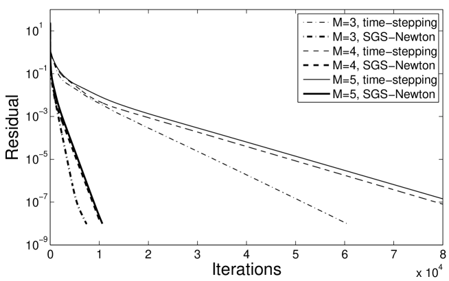
Figure 1: Convergence history on a uniform grid with $N=1024$ of the planar Couette flow for $\mathit{Kn}=0.1199$, $u^{W}=1.2577$.

In view of that the exact solution for the local problem (23) is not necessary, an improvement in efficiency is obtained by additional criteria for Algorithm 1. In our implementation, the local Newton iteration also stops if the local residual decreases in half or the maximum steps, set as 5, is reached. An even essential improvement in efficiency is multigrid acceleration by using the SGS-Newton iteration as smoother, which is described in the following section.

4 Multigrid Solver

Using the SGS-Newton iteration as smoother, the multigrid strategy we adopt is the nonlinear multigrid approach [16]. Besides the smoother, the main ingredients of a nonlinear multigrid solver are the coarse grid correction and the operators (restriction and prolongation) between the fine and coarse grids. In this section, we first consider a two-grid solver to give the coarse grid correction problem, and to construct the restriction and the prolongation operators. Then it is generalized to a complete multigrid algorithm by recursion. For convenience, we introduce subscripts $h$ and $H$ to denote operators and variables related to the fine and coarse grids, respectively.

4.1 Coarse grid correction

In contrast to the linear multigrid procedure which solves a correction equation for the coarse grid correction directly, the nonlinear multigrid procedure calculate the coarse grid solution first. As seen in the last section, let us re-written the fine grid problem resulting from (23) into a global form as

$$R_{h}(f_{h})=r_{h},$$ (32)

and suppose $\bar{f}_{h}$ is an approximate solution for the above problem. The corresponding coarse grid problem is given as

$$R_{H}(f_{H})=r_{H}\triangleq R_{H}(I_{h}^{H}\bar{f}_{h})+I_{h}^{H}\left(r_{h}-R_{h}(\bar{f}_{h})\right),$$ (33)

where $I_{h}^{H}$ is the restriction operator from the fine grid to the coarse grid, and $R_{H}(f_{H})$ is evaluated analogously to the fine grid counterpart $R_{h}(f_{h})$. It follows that (33) can be solved using the SGS-Newton iteration, and a solution $f_{H}$ is obtained by employing Algorithm 2. Then the fine grid solution $\bar{f}_{h}$ is corrected as

$$\hat{f}_{h}=\bar{f}_{h}+I_{H}^{h}\left(f_{H}-I_{h}^{H}\bar{f}_{h}\right),$$ (34)

where $I_{H}^{h}$ is the prolongation operator from the coarse grid to the fine grid.

4.2 Restriction and prolongation

In our implementation, the coarse grid is generated from the fine grid by a standard way, namely, the coarse grid point $x_{\scriptscriptstyle H,i}$ coincides with the fine grid point $x_{\scriptscriptstyle h,2i}$. Based on this, we construct the restriction operator $I_{h}^{H}$ locally, which means for any fine grid function $g_{\scriptscriptstyle h}$, its restriction $g_{\scriptscriptstyle H,i}$ on the $i$-th coarse grid cell $[x_{\scriptscriptstyle H,i},x_{\scriptscriptstyle H,i+1}]$, given by $g_{\scriptscriptstyle H}=I_{h}^{H}g_{\scriptscriptstyle h}$, is determined only by $g_{\scriptscriptstyle h,2i}$ and $g_{\scriptscriptstyle h,2i+1}$. The detailed construction of the restriction operator $I_{h}^{H}$ can be found in Appendix B, and we only show the final result here.

There are two grid variables in (33), the solution $\bar{f}_{h}$ and the residual $\bar{R}_{h}=r_{h}-R_{h}(\bar{f}_{h})$, which are required to be transferred on to the coarse grid using $I_{h}^{H}$. The restrictions $\bar{f}_{H,i}$ and $\bar{R}_{H,i}$ on the $i$-th coarse grid cell are constructed in the following steps

1. Compute $\bar{\boldsymbol{u}}_{\scriptscriptstyle H,i}$ and $\bar{\theta}_{H,i}$ from (48);

2. Project $\bar{f}_{h,2i}$, $\bar{f}_{h,2i+1}$, $\bar{R}_{h,2i}$ and $\bar{R}_{h,2i+1}$ into $\mathcal{F}_{M}(\bar{\boldsymbol{u}}_{\scriptscriptstyle H,i},\bar{\theta}_{H,i})$, then calculate $\bar{f}_{H,i,\alpha}$ and $\bar{R}_{H,i,\alpha}$ by the formula (52).

For the prolongation operator $I_{H}^{h}$, the simple identical operator is employed. Then the correction formula (34) is re-written as

$$\hat{f}_{h}=\delta\bar{f}_{h}+f_{H},$$ (35)

where $\delta\bar{f}_{h}=\bar{f}_{h}-I_{h}^{H}\bar{f}_{h}$. It is pointed out that the above formula includes the projection procedure to represent $\hat{f}_{h}$ in $\mathcal{F}_{M}(\hat{\boldsymbol{u}}_{\scriptscriptstyle h},\hat{\theta}_{h})$.

4.3 Overall algorithm

As the computation of the exact solution $f_{H}$ on the coarse grid by the SGS-Newton iteration is still cumbersome for a large number of $N_{H}$, the coarse grid problem (33) is solved recursively with the multigrid algorithm until the exact solution on the coarsest grid can be obtained cheaply. This results in a complete multigrid algorithm.

Now let us introduce subscripts $h_{k}$, $k=0,1,\ldots,K$ to denote operators and variables related to the $k$-th level grid, where $h_{0}$ and $h_{K}$ correspond to the coarsest and the finest grid, respectively. Then the $(k+1)$-th level multigrid iteration, denoted by $f_{h_{k}}^{n+1}=\text{NMG}(f_{h_{k}}^{n},r_{h_{k}},k)$, is given in the following algorithm.

Algorithm 3 (Nonlinear multigrid (NMG) iteration).

1. If $k=0$, call Algorithm 2 to have a solution as $f_{h_{0}}^{n+1}$; otherwise, go to the next step.

2. Pre-smoothing: perform $\nu_{1}$ smoothing steps using the SGS-Newton iteration to obtain a new approximation $\bar{f}_{h_{k}}$, that is, $\bar{f}_{h_{k}}=\emph{SGS-Newton}(f_{h_{k}}^{n},r_{h_{k}},\nu_{1})$.

3. Coarse grid correction:

   1. Compute the fine grid residual as $\bar{R}_{h_{k}}=r_{h_{k}}-R_{h_{k}}(\bar{f}_{h_{k}})$.

   2. Calculate the coarse grid approximation by the restriction operator $I_{h_{k}}^{h_{k-1}}$ as $\bar{f}_{h_{k-1}}=I_{h_{k}}^{h_{k-1}}\bar{f}_{h_{k}}$, and compute the difference $\delta\bar{f}_{h_{k}}$ with

      $$\delta\bar{f}_{h_{k},2i}=\bar{f}_{h_{k},2i}-\bar{f}_{h_{k-1},i},\quad\delta\bar{f}_{h_{k},2i+1}=\bar{f}_{h_{k},2i+1}-\bar{f}_{h_{k-1},i},\qquad i=0,1,\ldots,N_{h_{k-1}}.$$

   3. Calculate the right hand side of the coarse grid problem (33) as $r_{h_{k-1}}=I_{h_{k}}^{h_{k-1}}\bar{R}_{h_{k}}+R_{h_{k-1}}(\bar{f}_{h_{k-1}})$.

   4. Recursively call the multigrid algorithm (repeat $\gamma$ times with $\gamma=1$ for a so-called $V$-cycle, $\gamma=2$ for a $W$-cycle, and so on) as

      $$\tilde{f}_{h_{k-1}}=\emph{NMG}^{\gamma}(\bar{f}_{h_{k-1}},r_{h_{k-1}},k-1).$$

   5. Correct the fine grid solution by $\hat{f}_{h_{k}}=\delta\bar{f}_{h_{k}}+\tilde{f}_{h_{k-1}}$.

4. Post-smoothing: perform $\nu_{2}$ smoothing steps using the SGS-Newton iteration to obtain the new approximation as

   $$f_{h_{k}}^{n+1}=\emph{SGS-Newton}(\hat{f}_{h_{k}},r_{h_{k}},\nu_{2}).$$

The NMG solver is then obtained from Algorithm 2 where the SGS-Newton iteration is replaced by the above NMG iteration.

5 Numerical Examples

Two numerical examples, the planar Couette flow and the force driven Poiseuille flow, are presented in this section to illustrate the main features of the NMG solver described in previous section. In all tests below, a $V$-cycle NMG with smoothing steps $\nu_{1}=\nu_{2}=2$ is employed, and its level is chosen such that there are only four cells on the coarsest grid. With such a small grid, the solution can be obtained very cheaply by the SGS-Newton iteration, e.g., in most tests, only $30$ SGS-Newton iterations is enough to resolve the coarsest grid problem exactly at the beginning of the NMG iteration, and the steps of the SGS-Newton iteration is quickly decreased to 1 in successive NMG iterations.

For simplicity, the Prandtl number $\Pr$ is set as $2/3$, and we consider the solution of the dimensionless equation, which has the same form as (1) with the particle mass $m=1$. As mentioned in Section 2, the Maxwell boundary conditions for moment system derived in [7] are adopted. It is easy to show that such boundary conditions could not determine a unique solution for the steady-state moment system (12). For the time-stepping scheme, the additional initial condition is used to obtain the unique solution. However, since the classical Gauss-Seidel iteration is non-conservative, it is apparently that our NMG iteration using the SGS-Newton iteration as smoother is also non-conservative. This leads to a steady-state solution which is inconsistent with the time-stepping solution only for the density, even though the same initial condition is employed as the initial guess in our NMG solver. In order to converge towards the same steady-state solution as the time-stepping scheme, the solution is corrected as [27] at each NMG iterative step, that is,

$$f^{\text{new}}\leftarrow\frac{\displaystyle\int f^{0}(x,\boldsymbol{\xi})\,\mathrm{d}\boldsymbol{\xi}\,\mathrm{d}x}{\displaystyle\int f^{\text{new}}(x,\boldsymbol{\xi})\,\mathrm{d}\boldsymbol{\xi}\,\mathrm{d}x}f^{\text{new}}=\frac{\sum\limits_{i=0}^{N-1}\rho_{i}^{0}\Delta x_{i}}{\sum\limits_{i=0}^{N-1}\rho_{i}^{\text{new}}\Delta x_{i}}f^{\text{new}}.$$ (36)

The above correction is sufficient to recover the consistent steady-state solution.

All our computations are performed on Linux operating system on an Xeon workstation with a quad-core processor and core speed 2.93GHz. The global tolerance Tol is set as $10^{-8}$.

5.1 The planar Couette flow

We first consider a force-free benchmark problem, namely, the planar Couette flow. To compare with the solution of the moment system using the time-stepping scheme in [8], we use the same data and parameters in our tests. The gas of argon lies between two plates parallel to the $yz$-plane with a distance of $L=1$. These two plates have the same temperature of $\theta^{W}=1$, and one plate is stationary while the other moves with a constant velocity $u^{W}$ in the $y$ direction. The dimensionless collision frequency $\nu$ is given as

$$\nu=\sqrt{\frac{\pi}{2}}\frac{\Pr}{\mathit{Kn}}\rho\theta^{1-w},$$ (37)

where $\mathit{Kn}$ is the Knudsen number, and the viscosity $\mu$ used in (3) is assumed as a function directly proportional to $w$ power of temperature, i.e., $\mu\propto\theta^{w}$. For the gas of argon, we have $w=0.81$. These settings are actually the same as in [27], whose solution of the non-dimensionless Boltzmann equation using the discrete velocity method is utilized as a reference of the solution of the moment system.

In this example, all the computations begin with a global equilibrium with

$$\rho^{0}(x)=1,\quad\boldsymbol{u}^{0}(x)=0,\quad\theta^{0}(x)=1.$$ (38)

Since our NMG solver delivers exactly the same steady-state solution as the time-stepping scheme in [8], where the solution of the moment system for this example has been presented and compared with the reference solution, we omit any discussion on the accuracy of our solution, and only focus on the efficiency of the NMG solver. As an example, the steady-state solution for $\mathit{Kn}=0.1199$ and $u^{W}=1.2577$ on a uniform grid with $N=2048$ is displayed in Figure 2, compared with the reference solution. The convergence history in terms of NMG iterations for this case is presented in Figure 3, which shows the efficiency and robustness of the NMG solver for various $M$.

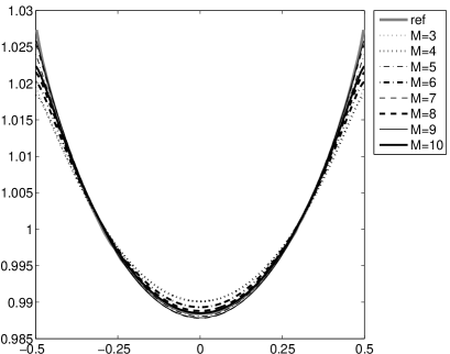
(a) Density, $\rho$

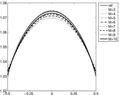
(b) Temperature, $\theta$

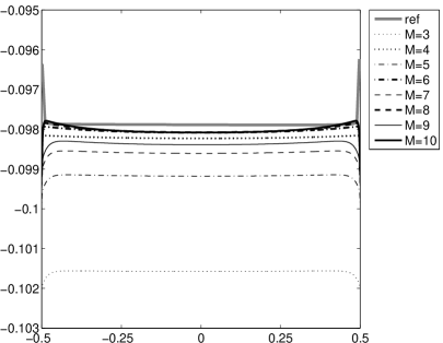
(c) Shear stress, $\sigma_{12}$

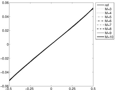
(d) Heat flux, $q_{1}$

Figure 2: Solution of the Couette flow for $\mathit{Kn}=0.1199$ and $u^{W}=1.2577$ on a uniform grid with $N=2048$.

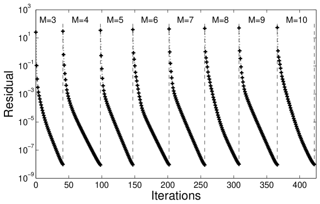
Figure 3: Convergence history of the Couette flow with $\mathit{Kn}=0.1199$ and $u^{W}=1.2577$ on a uniform grid with $N=2048$.

Now let us consider the behavior of the NMG solver with respect to the grid size. We first test the Couette flow for $\mathit{Kn}=0.1199$ and $u^{W}=1.2577$ on a uniform refined meshes sequence. As shown in Table 1 for the number of NMG iterations, and in Figure 4 for convergence history with $M=3$ and total iterations in terms of grid size, the NMG solver works well on the uniform mesh. Although the total iterations increase as the grid size increases, the rate of increase is much slower than the single grid solver such as the SGS-Newton iteration and the time-stepping scheme, which are well known that double the iterations as the grid size doubles. This indicates that the NMG solver is substantially more efficient than the single grid solver on finer grids. It is also shown in Figure 4 (right) that the solution of the moment system for odd $M$ converge faster than the solution for even $M$ as grid size increases.

$N$		$2^{7}$	$2^{8}$	$2^{9}$	$2^{10}$	$2^{11}$	$2^{12}$	$2^{13}$
Iterations	$M=3$	16	19	23	30	41	56	75
	$M=4$	18	23	31	41	57	81	116
	$M=5$	19	22	28	37	49	66	89
	$M=6$	20	23	29	38	55	79	114

Table 1: Iterations of the Couette flow for $\mathit{Kn}=0.1199$ and $u^{W}=1.2577$ on different uniform grids.

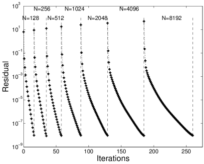
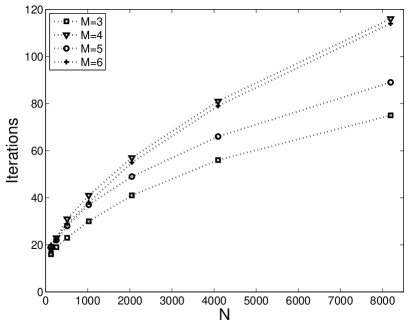
Figure 4: Convergence history ($M=3$, left) and iterations (right) of the Couette flow for $\mathit{Kn}=0.1199$ and $u^{W}=1.2577$ on different uniform grids.

Then we test the same case on a sequence of non-uniform meshes generated by the inverse hyperbolic sine function as

$$x_{i}=x_{0}+\frac{\sinh^{-1}(-5+\frac{10i}{N})-\sinh^{-1}(-5)}{\sinh^{-1}(5)-\sinh^{-1}(-5)},\quad i=0,1,\ldots,N.$$ (39)

This mesh is a particular setup for resolving the Knudsen layer around the boundary. As can be seen in Table 2 and Figure 5, the NMG solver behaves similar features on these meshes. It is clear that these are meshes seriously deviating from a quasi-uniform mesh, indicating the NMG solver is quite stable.

$N$		$2^{7}$	$2^{8}$	$2^{9}$	$2^{10}$	$2^{11}$	$2^{12}$	$2^{13}$
Iterations	$M=3$	19	25	34	46	61	81	110
	$M=4$	22	29	41	59	85	123	175
	$M=5$	20	27	36	49	66	91	126
	$M=6$	21	27	39	58	84	121	172

Table 2: Iterations of the Couette flow for $\mathit{Kn}=0.1199$ and $u^{W}=1.2577$ on non-uniform grids.

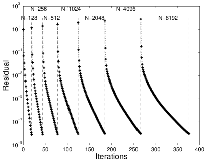
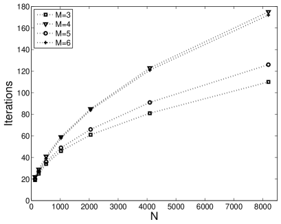
Figure 5: Convergence history ($M=3$, left) and iterations (right) of the Couette flow for $\mathit{Kn}=0.1199$ and $u^{W}=1.2577$ on non-uniform grids.

At last, we examine the performance of the NMG solver for different Knudsen numbers and $u^{W}$. Again similar convergence histories are obtained, and the total NMG iterations are presented in Table 3. As the time-stepping scheme, the NMG solver converges slower in both cases for $\mathit{Kn}=0.01199$ and $\mathit{Kn}=1.199$ than the case for $\mathit{Kn}=0.1199$. However, there is still a substantial gain in efficiency in comparison to the single grid solver. For large plate velocity of $u^{W}=4.1923$, the NMG solver converges a little slower than the case $u^{W}=1.2577$.

$u^{W}$	$1.2577$		$4.1923$
$\mathit{Kn}$	$0.01199$	$1.199$	$0.1199$
Iterations	115	120	52

Table 3: Iterations of the Couette flow for various Knudsen numbers and $u^{W}$ on a uniform grid with $N=2048$ and $M=3$.

5.2 Force driven Poiseuille flow

Next we consider the force driven Poiseuille flow which is also frequently investigated in the literatures [31, 7, 30]. For this example, the gas lies between two stationary plates parallel to the $yz$-plane with a distance of $L=1$, and two plates have the same temperature of $\theta^{W}=1$. In contrast to the Couette flow, the Poiseuille flow is driven by an external constant force, which is set as $\boldsymbol{F}=(0,0.2555,0)^{T}$ in our tests. Additionally, the collision frequency $\nu$ is given by the hard sphere model as

$$\nu=\frac{16}{5}\sqrt{\frac{\theta}{2\pi}}\frac{\Pr}{\mathit{Kn}}\rho,$$ (40)

and the Knudsen number $\mathit{Kn}=0.1$ is considered. The computations also begin with the global equilibrium (38) as the Couette flow. For these settings of the Poiseuille flow, the solution of the Boltzmann equation using the direct simulation of Monte Carlo (DSMC) was investigated in [31], and the solution of the Boltzmann equation with the Shakhov collision term using the NR$xx$ method was considered in [7]. Here we present the solution of the hyperbolic moment system for the Boltzmann equation with the ES-BGK collision term in Figure 6.

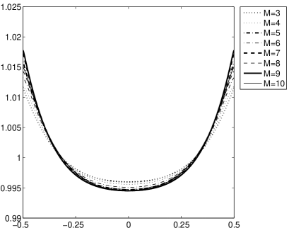
(a) Density, $\rho$

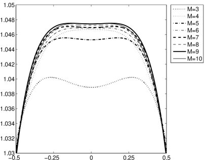
(b) Temperature, $\theta$

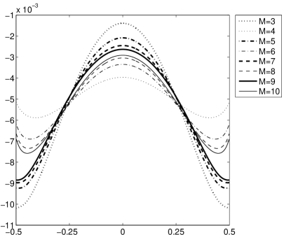
(c) Normal stress, $\sigma_{11}$

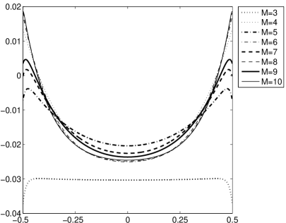
(d) Heat flux, $q_{2}$

Figure 6: Solution of the force driven Poiseuille flow.

We still omit the discussion on the solution in comparison with the solution given in [7, 31], and focus on the efficiency of the NMG solver. The convergence histories for various $M$ on a uniform grid with $N=2048$ and for $M=3$ on a uniform refined grids series are shown in Figure 7 and Figure 8 (left), respectively, while the corresponding number of NMG iterations can be found in Table 4. The total iterations in terms of grid size are presented in Figure 8 (right). As expected, the results show the similar convergence rates for all simulations as the force-free Couette flow, which implies a great improvement in efficiency compared with the single grid solver.

It is also seen in Figure 7 that the convergence rate slows down quickly in the last few iterations for $M=10$. Similar situations occur in simulations of the Couette flow with large $M$ or large $u^{W}$. The reason might be that in these cases the amount of residual reduced by the smoothing steps is in the same order as the error introduced by transferring the solution between two successive grids. Just increasing the smoothing steps can preserve the convergence rate during the total iterations. However, the use of large smoothing steps during the total iterations is not preferable in considering the computational cost. In fact, the case of the smoothing steps $\nu_{1}=\nu_{2}=1$ is more efficient than the case of $\nu_{1},\nu_{2}>1$ if it can preserve the convergence rate. Consequently, an adaptive choice of the smoothing steps might be considered to save the computational cost while maintaining the convergence rate.

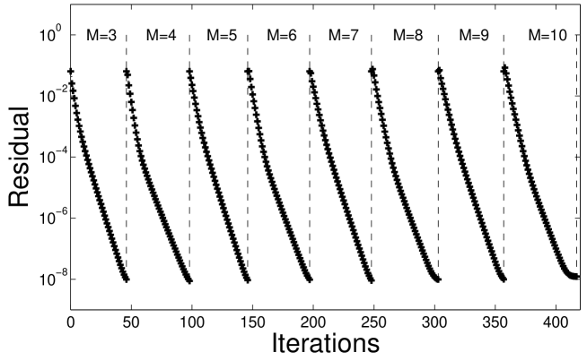
Figure 7: Convergence history of the force driven Poiseuille flow on the uniform grid with $N=2048$.

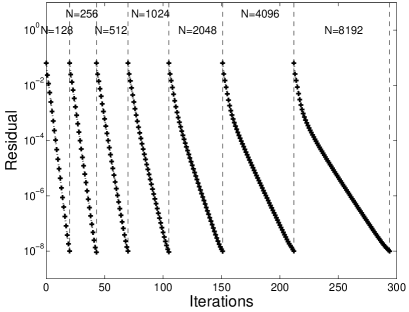
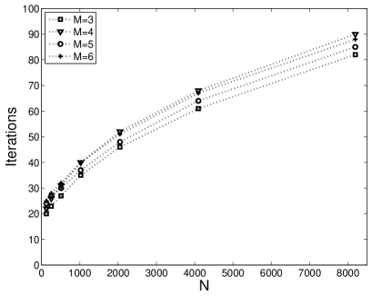
Figure 8: Convergence history ($M=3$, left) and iterations (right) of the force driven Poiseuille flow on a uniform grids series.

$N$		$2^{7}$	$2^{8}$	$2^{9}$	$2^{10}$	$2^{11}$	$2^{12}$	$2^{13}$
Iterations	$M=3$	20	23	27	35	46	61	82
	$M=4$	22	26	31	40	52	68	90
	$M=5$	24	27	30	37	48	64	85
	$M=6$	25	28	32	40	51	67	88

Table 4: Iterations of the force driven Poiseuille flow on a uniform grids series.

6 Concluding remarks

An efficient and robust nonlinear multigrid solver has been developed for the hyperbolic moment system derived for the steady-state Boltzmann equation with ES-BGK collision term. The moment system is discretized using the unified framework of the NR$xx$ method such that our solver is also unified for the system with moments up to arbitrary order. A nonlinear iterative method, namely, SGS-Newton iteration, is presented to solve the resulting discretized system on a single grid level. It is then accelerated drastically by putting itself as smoother into a routine nonlinear multigrid procedure. The numerical experiments on two benchmark problems demonstrate the efficiency and the robustness of our NMG solver.

Although we have considered only the moment system for the Boltzmann equation with ES-BGK collision term, the implementation of the proposed NMG solver is clearly not restricted to this collision model. It is trivial to extend our NMG solver to the BGK model since it is a special case of the ES-BGK model with $\Pr=1$. For the Shakhov model, the extension is still quite simple with the expansion of the collision term given in [7].

The extension of the NMG solver to high spatial dimensional case is under our current study and will be reported elsewhere.

Appendices

Appendix A Computation of the parameter $\hat{\tau}$

Suppose the distribution function $g$ belongs to the space $\mathcal{F}_{M}(\boldsymbol{u},\theta)$, where the relation (11) holds for its coefficients $g_{\alpha}$. When approximate $g$ in another space $\mathcal{F}_{M}(\boldsymbol{u}^{\prime},\theta^{\prime})$, the corresponding coefficients, denoted by $g_{\alpha}^{\prime}$, would not satisfy (11) usually. However, similar relation can be deduced from (6), which is given as

$$\begin{aligned} &\rho=g_{0}^{\prime},\\ &\rho(\boldsymbol{u}-\boldsymbol{u}^{\prime})=(g_{e_{1}}^{\prime},g_{e_{2}}^{\prime},g_{e_{3}}^{\prime})^{T},\\ &\rho|\boldsymbol{u}-\boldsymbol{u}^{\prime}|^{2}+3\rho(\theta-\theta^{\prime})=2\sum_{d=1}^{3}g_{2e_{d}}^{\prime}.\end{aligned}$$ (41)

The last two equations of (41) indicate

$$\theta=\frac{2\sum_{d=1}^{3}g_{2e_{d}}^{\prime}-\sum_{d=1}^{3}(g_{e_{d}}^{\prime})^{2}/\rho}{3\rho}+\theta^{\prime}.$$ (42)

Now corresponding to the step of updating solution by (30) in the local Newton iteration (Algorithm 1), we have

$$\begin{aligned} &\rho=g_{0}^{\prime}=f_{i,0}^{(m)}+\tau\Delta f_{i,0}^{(m)},\qquad\boldsymbol{u}^{\prime}=\boldsymbol{u}_{i}^{(m)},\qquad\theta^{\prime}=\theta_{i}^{(m)},\\ &g_{e_{d}}^{\prime}=\tau\Delta f_{i,e_{d}}^{(m)},\quad d=1,2,3,\qquad\sum_{d=1}^{3}g_{2e_{d}}^{\prime}=\tau\sum_{d=1}^{3}\Delta f_{i,2e_{d}}^{(m)}.\end{aligned}$$ (43)

Substituting the above equations into (42) immediately yields

$$\theta=\frac{2\tau\sum_{d=1}^{3}\Delta f_{i,2e_{d}}^{(m)}-\tau^{2}\sum_{d=1}^{3}(\Delta f_{i,e_{d}}^{(m)})^{2}/(f_{i,0}^{(m)}+\tau\Delta f_{i,0}^{(m)})}{3(f_{i,0}^{(m)}+\tau\Delta f_{i,0}^{(m)})}+\theta_{i}^{(m)}.$$ (44)

In our implementation, the positivity of the density and the temperature are preserved during the iterations, that is,

$$\rho\geq\bar{\rho}>0,\qquad\theta\geq\bar{\theta}>0,$$

where $\bar{\rho}$, $\bar{\theta}$ are the given lower bounds of the density and the temperature respectively.

For the positivity of the density, we have

$$0<\tau\leq\frac{\bar{\rho}-f_{i,0}^{(m)}}{\Delta f_{i,0}^{(m)}},$$ (45)

if $\Delta f_{i,0}^{(m)}<0$. Otherwise, the density is always positive for $\tau>0$.

For the positivity of the temperature, we deduce from (44) that

$$A\tau^{2}+B\tau+C\leq 0,$$ (46)

where

$$A=\sum_{d=1}^{3}\left(\Delta f_{i,e_{d}}^{(m)}\right)^{2}-2\Delta f_{i,0}^{(m)}\sum_{d=1}^{3}\Delta f_{i,2e_{d}}^{(m)}-(\theta_{i}^{(m)}-\bar{\theta})\left(\Delta f_{i,0}^{(m)}\right)^{2},$$

$$B=-2f_{i,0}^{(m)}\left(\sum_{d=1}^{3}\Delta f_{2e_{d}}^{(m)}+\Delta f_{i,0}^{(m)}(\theta_{i}^{(m)}-\bar{\theta})\right),\qquad C=-(f_{i,0}^{(m)})^{2}(\theta_{i}^{(m)}-\bar{\theta}).$$

It is trivial to solve the above inequality, and the solution is given as

1. $0<\tau\leq-\frac{C}{B}$ if $A=0$, $B>0$.

2. $0<\tau\leq\frac{-B+\sqrt{B^{2}-4AC}}{2A}$, if $A>0$, $B^{2}-4AC>0$ or $A<0$, $B>0$, $B^{2}-4AC>0$.

3. Otherwise, $\tau>0$.

Finally, the parameter $\hat{\tau}$ is obtained such that the above inequalities (45) and (46) hold for $\tau$.

Appendix B Construction of the restriction operator $I_{h}^{H}$

For any fine grid function $g_{\scriptscriptstyle h}$ with $g_{\scriptscriptstyle h,i}\in\mathcal{F}_{M}(\boldsymbol{u}_{\scriptscriptstyle h,i},\theta_{h,i})$, denote its restriction $I_{h}^{H}g_{\scriptscriptstyle h}$ by $g_{\scriptscriptstyle H}$. Obviously, it is enough to construct $g_{\scriptscriptstyle H,i}$ on the $i$-th coarse grid cell $[x_{\scriptscriptstyle H,i},x_{\scriptscriptstyle H,i+1}]$. Suppose $g_{\scriptscriptstyle H,i}$ belongs to $\mathcal{F}_{M}(\boldsymbol{u}_{\scriptscriptstyle H,i},\theta_{H,i})$, where $\boldsymbol{u}_{\scriptscriptstyle H,i}$ and $\theta_{H,i}$ are macroscopic velocity and temperature of the restriction $I_{h}^{H}f_{h}$ on the $i$-th coarse grid cell, in which $f_{h}$ is the fine grid solution for (32).

Due to the importance of conservation, $g_{\scriptscriptstyle H,i}$ is required to preserve this property. To be specific, the following equation

$$\int_{x_{H,i}}^{x_{H,i+1}}\int g_{\scriptscriptstyle H,i}(\boldsymbol{\xi})p(\boldsymbol{\xi})\,\mathrm{d}\boldsymbol{\xi}\,\mathrm{d}x=\int_{x_{h,2i}}^{x_{h,2i+1}}\int g_{\scriptscriptstyle h,2i}(\boldsymbol{\xi})p(\boldsymbol{\xi})\,\mathrm{d}\boldsymbol{\xi}\,\mathrm{d}x+\int_{x_{h,2i+1}}^{x_{h,2i+2}}\int g_{\scriptscriptstyle h,2i+1}(\boldsymbol{\xi})p(\boldsymbol{\xi})\,\mathrm{d}\boldsymbol{\xi}\,\mathrm{d}x$$ (47)

should hold for any polynomial $p(\boldsymbol{\xi})$ of degree no more than $M$. To evaluate an arbitrary restriction $g_{\scriptscriptstyle H,i}$, one should first calculate $\boldsymbol{u}_{\scriptscriptstyle H,i}$ and $\theta_{H,i}$. To this end, replacing $g_{\scriptscriptstyle H}$ and $g_{\scriptscriptstyle h}$ by the solution $f_{H}$ and $f_{h}$ respectively, and employing (6), we have

$$\begin{aligned} \rho_{\scriptscriptstyle H,i}\Delta x_{\scriptscriptstyle H,i}=&~{}\rho_{\scriptscriptstyle h,2i}\Delta x_{\scriptscriptstyle h,2i}+\rho_{\scriptscriptstyle h,2i+1}\Delta x_{\scriptscriptstyle h,2i+1},\\ \rho_{\scriptscriptstyle H,i}\boldsymbol{u}_{\scriptscriptstyle H,i}\Delta x_{\scriptscriptstyle H,i}=&~{}\rho_{\scriptscriptstyle h,2i}\boldsymbol{u}_{\scriptscriptstyle h,2i}\Delta x_{\scriptscriptstyle h,2i}+\rho_{\scriptscriptstyle h,2i+1}\boldsymbol{u}_{\scriptscriptstyle h,2i+1}\Delta x_{\scriptscriptstyle h,2i+1},\\ \left(\rho_{\scriptscriptstyle H,i}\boldsymbol{u}_{\scriptscriptstyle H,i}^{2}+3\rho_{\scriptscriptstyle H,i}\theta_{H,i}\right)\Delta x_{\scriptscriptstyle H,i}=&~{}\Delta x_{\scriptscriptstyle h,2i}\left(\rho_{\scriptscriptstyle h,2i}\boldsymbol{u}_{\scriptscriptstyle h,2i}^{2}+3\rho_{\scriptscriptstyle h,2i}\theta_{h,2i}\right)\\ &+\Delta x_{\scriptscriptstyle h,2i+1}\left(\rho_{\scriptscriptstyle h,2i+1}\boldsymbol{u}_{\scriptscriptstyle h,2i+1}^{2}+3\rho_{\scriptscriptstyle h,2i+1}\theta_{h,2i+1}\right).\end{aligned}$$ (48)

After computing $\boldsymbol{u}_{\scriptscriptstyle H,i}$, $\theta_{H,i}$ from the above equations, we employ the transformation [6] to project $g_{\scriptscriptstyle h,2i}$ and $g_{\scriptscriptstyle h,2i+1}$ into $\mathcal{F}_{M}(\boldsymbol{u}_{\scriptscriptstyle H,i},\theta_{H,i})$, denoted by $\tilde{g}_{\scriptscriptstyle h,2i}$ and $\tilde{g}_{\scriptscriptstyle h,2i+1}$ respectively. As the transformation is conservative, (47) is re-written as

$$\begin{aligned} \int_{x_{H,i}}^{x_{H,i+1}}\int g_{\scriptscriptstyle H,i}(\boldsymbol{\xi})p(\boldsymbol{\xi})\,\mathrm{d}\boldsymbol{\xi}\,\mathrm{d}x=&\int_{x_{h,2i}}^{x_{h,2i+1}}\int\tilde{g}_{\scriptscriptstyle h,2i}(\boldsymbol{\xi})p(\boldsymbol{\xi})\,\mathrm{d}\boldsymbol{\xi}\,\mathrm{d}x\\ &+\int_{x_{h,2i+1}}^{x_{h,2i+2}}\int\tilde{g}_{\scriptscriptstyle h,2i+1}(\boldsymbol{\xi})p(\boldsymbol{\xi})\,\mathrm{d}\boldsymbol{\xi}\,\mathrm{d}x.\end{aligned}$$ (49)

Now let

$$p_{\alpha}(\boldsymbol{\xi})=\mathcal{H}_{\theta_{H,i},\alpha}\left(\frac{\boldsymbol{\xi}-\boldsymbol{u}_{\scriptscriptstyle H,i}}{\sqrt{\theta_{H,i}}}\right)\exp\left(\frac{|\boldsymbol{\xi}-\boldsymbol{u}_{\scriptscriptstyle H,i}|^{2}}{2\theta_{H,i}}\right),\quad|\alpha|\leq M.$$ (50)

It is trivial to show that $\{p_{\alpha}(\boldsymbol{\xi})\}_{|\alpha|\leq M}$ forms a complete orthogonal basis of the polynomial space of degree no more than $M$. Substituting (50) into (49), and employing the orthogonality of the basis, we deduce

$$\int_{x_{H,i}}^{x_{H,i+1}}g_{\scriptscriptstyle H,i,\alpha}\,\mathrm{d}x=\int_{x_{h,2i}}^{x_{h,2i+1}}\tilde{g}_{\scriptscriptstyle h,2i,\alpha}\,\mathrm{d}x+\int_{x_{h,2i+1}}^{x_{h,2i+2}}\tilde{g}_{\scriptscriptstyle h,2i+1,\alpha}\,\mathrm{d}x,\quad|\alpha|\leq M,$$ (51)

which follows that

$$g_{\scriptscriptstyle H,i,\alpha}=\frac{\tilde{g}_{\scriptscriptstyle h,2i,\alpha}\Delta x_{\scriptscriptstyle h,2i}+\tilde{g}_{\scriptscriptstyle h,2i+1,\alpha}\Delta x_{\scriptscriptstyle h,2i+1}}{\Delta x_{\scriptscriptstyle H,i}},\quad|\alpha|\leq M.$$ (52)

References

• [1] P.ย L. Bhatnagar, E.ย P. Gross, and M.ย Krook. A model for collision processes in gases. I. small amplitude processes in charged and neutral one-component systems. Phys. Rev., 94(3):511โ€“525, 1954.
• [2] A.ย Brandt and O.ย E. Livne. Multigrid Techniques: 1984 Guide with Applications to Fluid Dynamics. Classics in Applied Mathematics. SIAM, revised edition, 2011.
• [3] Z.ย Cai, Y.ย Fan, and R.ย Li. Globally hyperbolic regularization of Gradโ€™s moment system in one dimensional space. Comm. Math Sci., 11(2):547โ€“571, 2013.
• [4] Z.ย Cai, Y.ย Fan, and R.ย Li. Globally hyperbolic regularization of Gradโ€™s moment system. Comm. Pure Appl. Math., 67(3):464โ€“518, 2014.
• [5] Z.ย Cai, Y.ย Fan, R.ย Li, T.ย Lu, and Y.ย Wang. Quantum hydrodynamics models by moment closure of wigner equation. J. Math. Phys., 53:103503, 2012.
• [6] Z.ย Cai and R.ย Li. Numerical regularized moment method of arbitrary order for Boltzmann-BGK equation. SIAM J. Sci. Comput., 32(5):2875โ€“2907, 2010.
• [7] Z.ย Cai, R.ย Li, and Z.ย Qiao. NR$xx$ย  simulation of microflows with Shakhov model. SIAM J. Sci. Comput., 34(1):A339โ€“A369, 2012.
• [8] Z.ย Cai, R.ย Li, and Z.ย Qiao. Globally hyperbolic regularized moment method with applications to microflow simulation. Computers and Fluids, 81:95โ€“109, 2013.
• [9] Z.ย Cai, R.ย Li, and Y.ย Wang. An efficient NR$xx$ย  method for Boltzmann-BGK equation. J. Sci. Comput., 50(1):103โ€“119, 2012.
• [10] Z.ย Cai, R.ย Li, and Y.ย Wang. Numerical regularized moment method for high Mach number flow. Commun. Comput. Phys., 11(5):1415โ€“1438, 2012.
• [11] Z.ย Cai, R.ย Li, and Y.ย Wang. Solving Vlasov equation using NR$xx$ย  method. To appear in SIAM J. Sci. Comput., 2012.
• [12] Z.-N. Cai, Y.-W. Fan, and R.ย Li. On hyperbolicity of 13-moment system. arXiv:1401.7523, 2013.
• [13] S.ย Chapman and T.ย G. Cowling. The Mathematical Theory of Non-uniform Gases, Third Edition. Cambridge University Press, 1990.
• [14] M.ย H. Ernst. Nonlinear model โ€” Boltzmann equations and exact solutions. Phys. Rep., 78(1):1โ€“171, 1981.
• [15] H.ย Grad. On the kinetic theory of rarefied gases. Comm. Pure Appl. Math., 2(4):331โ€“407, 1949.
• [16] W.ย Hackbusch. Multi-Grid Methods and Applications. Springer-Verlag, Berlin, 1985. second printing 2003.
• [17] L.ย H. Holway. New statistical models for kinetic theory: Methods of construction. Phys. Fluids, 9(1):1658โ€“1673, 1966.
• [18] G.ย H. Hu, R.ย Li, and T.ย Tang. A robust high-order residual distribution type scheme for steady Euler equations on unstructured grids. J. Comput. Phys., 229:1681โ€“1697, 2010.
• [19] G.ย H. Hu, R.ย Li, and T.ย Tang. A robust WENO type finite volume solver for steady Euler equations on unstructured grids. Commun. Comput. Phys., 9(3):627โ€“648, 2011.
• [20] Z.ย Hu, , R.ย Li, T.ย Lu, Y.ย Wang, and W.ย Yao. Simulation of an $n^{+}$-$n$-$n^{+}$ diode by using globally-hyperbolically-closed high-order moment models. J. Sci. Comput., accepted for publication, 2013.
• [21] R.ย Li, X.ย Wang, and W.-B. Zhao. A multigrid block LU-SGS algorithm for Euler equations on unstructured grids. Numer. Math. Theor. Meth. Appl., 1(1):92โ€“112, 2008.
• [22] D.ย J. Mavriplis. On convergence acceleration techniques for unstructured meshes. AIAA Paper 98-2966, 1998.
• [23] D.ย J. Mavriplis. An assessment of linear versus nonlinear multigrid methods for unstructured mesh solvers. J. Comput. Phys., 175:302โ€“325, 2002.
• [24] D.ย J. Mavriplis. Multigrid solution of the steady-state lattice Boltzmann equation. Computers and Fluids, 35:793โ€“804, 2006.
• [25] J.ย Clerk Maxwell. On stresses in rarefied gases arising from inequalities of temperature. Proc. R. Soc. Lond., 27(185โ€“189):304โ€“308, 1878.
• [26] L.ย Mieussens. Discrete velocity model and implicit scheme for the BGK equation of rarefied gas dynamics. Math. Models Methods Appl. Sci., 10(8):1121โ€“1149, 2000.
• [27] L.ย Mieussens and H.ย Struchtrup. Numerical comparison of Bhatnagar-Gross-Krook models with proper Prandtl number. Phys. Fluids, 16(8):2797โ€“2813, 2004.
• [28] I.ย Mรผller and T.ย Ruggeri. Rational Extended Thermodynamics, Second Edition, volumeย 37 of Springer tracts in natural philosophy. Springer-Verlag, New York, 1998.
• [29] E.ย M. Shakhov. Generalization of the Krook kinetic relaxation equation. Fluid Dyn., 3(5):95โ€“96, 1968.
• [30] K.ย Xu, H.ย Liu, and J.ย Jiang. Multiple-temperature model for continuum and near continuum flows. Phys. Fluids, 19(1):016101, 2007.
• [31] Y.ย Zheng, A.ย L. Garcia, and B.ย J. Alder. Comparison of kinetic theory and hydrodynamics for Poiseuille flow. J. Stat. Phys., 109(3โ€“4):495โ€“505, 2002.