Quantum Landau-Lifshitz-Bloch equation and its comparison with the classical case

Abstract

The detailed derivation of the quantum Landau-Lifshitz-Bloch (qLLB) equation for simple spin-flip scattering mechanisms based on spin-phonon and spin-electron interactions is presented and the approximations are discussed. The qLLB equation is written in the form, suitable for comparison with its classical counterpart. The temperature dependence of the macroscopic relaxation rates is discussed for both mechanisms. It is demonstrated that the magnetization dynamics is slower in the quantum case than in the classical one.

I Introduction

The Landau-Lifshitz-Bloch (LLB) equation has recently received a lot of attention as a high-temperature extension of the classical micromagnetism. Chubykalo ; Lebecki The use of the LLB-based micromagnetism is progressively becoming more popular due to the appearance of novel high-temperature magnetic applications. The LLB formalism has been successfully used to model the heat-assisted magnetic recording, McDaniel ; Finnochio high-temperature spin-torque dynamics, Schieback spin-caloritronics Hinzke and laser-induced magnetization dynamics. AtxitiaNi ; Vahaplar Apart from their fundamental interest, these applications are very appealing from technological perspectives that range from energy saving strategies to the increase of the speed of the magnetization switching. Particularly, in the field of femtosecond optomagnetism, KirilyukRMP2010 where a sub-ps demagnetization can be induced by the ultrafast heating produced by a femtosecond laser pulse,Ostler the LLB equation has recommended itself as an useful approach. This is because it correctly describes the longitudinal magnetization relaxation in the strong internal exchange field, the key property of the magnetization dynamics at the timescale below 1 ps. AtxitiaNi ; AtxitiaQ ; Vahaplar Although the same characteristics have been proven to be reproduced by atomistic many-body approach, Kazantseva the use of the LLB micromagnetism for modeling purposes has some advantages: (i) the possibility to perform large scale modeling, for example, thermally-induced domain wall motion in much larger nanostructures Hinzke and (ii) analytical derivation of, for instance, the domain wall mobility quantumLLB or the demagnetization time scales. AtxitiaQ ; Nieves

Up to now, most of works used the classical version of the LLB equation which was derived starting from a Heisenberg spin model and the Landau-Lifshitz equation for classical atomic spins. classicalLLB This has made the classical LLB approach very popular since a direct comparison between the LLB and the atomistic simulations is therefore possible. Chubykalo ; Kazantseva However, the classical atomistic simulations mean effectively localized magnetic moments and correspond to the infinite spin number $S\rightarrow\infty$. As a consequence, the magnetization versus temperature curve follows a Langevin function rather than the Brillouin function which has been shown to fit better for ferromagnetic metals,Culity such as Ni and Co with $S=1/2$, Fe with $S=3/2$ and Gd with $S=7/2$. In principle, the classical approximation seems hard to justify in the magnetic materials commonly used for ultrafast magnetization dynamics measurements, such as ferromagnetic metals, because of the delocalized nature of the relevant electrons responsible for the magnetic properties. However, recent works which compare laser-induced magnetization dynamics experiments in metals with atomistic spin modelsVahaplar ; Radu ; Ostler as well as with their macroscopic counterpart - the classical LLB modelVahaplar ; AtxitiaNi - have proven that both models are very successful in the description and understanding of this phenomenon.

Similarly, the macroscopic three temperature model (M3TM), Koopmans ; Schellekens has also been successfully used in the description of femtomagnetism experiments. The M3TM assumes a collection of two level spin systems and uses a simple self-consistent Weiss mean-field model to evaluate the macroscopic magnetization. In the resulting system, importantly, the energy separation between levels is determined by a dynamical exchange interaction, similar to the LLB equation, which can be interpreted as a feedback effect to allow the correct account for the high temperature spin fluctuations. MuellerPRL2013 This consideration turns out to be a fundamental ingredient for the correct description of the ultrafast demagnetization in ferromagnets which suggests that the correct account for non-equilibrium thermodynamics is probably more important than the correct band structure. More recently, an alternative model to the M3TM and the LLB models, the so-called self-consistent Bloch (SCB) equationSCBloch which uses a quantum kinetic approach with the instantaneous local equilibrium approximation within the molecular field approximation (MFA), has been suggested.

Both the M3TM and SCB models can account for the quantum nature of magnetism whereas the atomistic approach and the classical LLB equation can not. However, the LLB model is not limited to the classical equation since there exists also the quantum version of the LLB equation. The quantum LLB equation (qLLB)quantumLLB has been derived even earlier than the classical one.classicalLLB The derivation is based on the density matrix approach for the spin operators, similar to the SCB model, and uses a dynamical exchange interaction within the MFA, similar to the M3TM model. One of the aims of the present paper is to study in more depth and to generalize the derivation of the qLLB equation in order to clarify its use for the ultrafast dynamics. We also aim to show that it contains both SCB and M3TM equations for $S=1/2$. Moreover, the qLLB equation has been barely investigated for numerical purposes. One of the reasons for that is mentioned above: the classical LLB equation allows the comparison with the atomistic simulations and, thus, its conclusions can be always checked. Another reason is the fact that the derivation has been made for the spin-phonon interaction mechanism which historically has been thought as the main contribution to the magnetization damping. This mechanism is important for ps-ns applications at high temperatures such as spincaloritronics. Recent experiment also explore the possibility to excite magnetization dynamics by acoustic pulses in picosecond range Scherbakov (THz excitation) where the phonon mechanism is the predominant one.Kim However, for the laser-induced magnetization dynamics where the spin-flips occur mainly due to the electron scattering, its relevance is marginal. Thus, in this work we also derive the qLLB equation by considering a simple spin-electron interaction as a source for magnetic relaxation.

The article is organized as follows. In section II we briefly outline the qLLB derivation. The derivation of the qLLB equation above the Curie temperature as well as for the simplest electron-”impurity” mechanism are presented. Comparatively to the original Garanin’s derivation, quantumLLB we discuss the approximations and put the qLLB equation in the form suitable for the comparison between the classical and the quantum cases. This allows us to relate the internal damping to microscopic scattering mechanisms. We also show the equivalence of the qLLB equation for $S=1/2$ with the SCB and the M3TM models. In section III we discuss the temperature dependence of the of the macroscopic longitudinal relaxation and the transverse damping as well as the internal microscopic coupling to the bath parameter within the two mechanisms. In section IV we present several numerical examples of the magnetization dynamics with the aim of comparison between the classical and the quantum cases. Finally, section V concludes the article and discusses possible extensions.

II Theoretical background for the quantum Landau-Lifshitz-Bloch equation

II.1 Basic assumptions for the qLLB equation with spin-phonon interaction

For completeness and for subsequent development, in this first subsection of the paper we summarize the main aspects and approximations of the derivation of the qLLB equation. quantumLLB The original derivation was done assuming a magnetic ion interacting weakly with a thermal phonon bath via direct and the second order (Raman) spin-phonon processes. The ferromagnetic interactions are taken into account in the mean-field approximation (MFA). The model Hamiltonian is written as:

$$\hat{\mathcal{H}}=\hat{\mathcal{H}}_{s}+\hat{\mathcal{H}}_{ph}+\hat{V}_{\textit{s-ph}},$$ (1)

where $\hat{\mathcal{H}}_{s}$ describes the spin system energy, $\hat{\mathcal{H}}_{ph}$ describes the phonon energy, $\hat{V}_{\textit{s-ph}}$ describes the spin-phonon interaction:

$$\hat{\mathcal{H}}_{s} = -\gamma\mathbf{H}^{\textrm{MFA}}\cdot\hat{\textbf{S}},$$

$$\hat{\mathcal{H}}_{ph} = \sum_{q}\hbar\omega_{q}\hat{a}_{q}^{\dagger}\hat{a}_{q},$$ (2)

$$\hat{V}_{\textit{s-ph}} = -\sum_{q}V_{q}(\mathbf{\bm{\eta}}\cdot\hat{\mathbf{S}})(\hat{a}_{q}^{\dagger}+\hat{a}_{-q})-\sum_{p,q}V_{p,q}(\mathbf{\bm{\eta}}\cdot\hat{\mathbf{S}})\hat{a}_{p}^{\dagger}\hat{a}_{q}.$$

In the expressions above $\hat{\textbf{S}}$ is the spin operator, $\hat{a}^{\dagger}_{q}$ ($\hat{a}_{q}$) is the creation (annihilation) operator which creates (annihilates) a phonon with frequency $\omega_{q}$ where $q$ stands for the wave vector k and the phonon polarization, and $\gamma=g\mu_{B}/\hbar$ is the gyromagnetic ratio where $g$ is the Landé g-factor, $\mu_{B}$ is the Bohr magneton and $\>\hbar$ is the reduced Planck constant.

The vector $\mathbf{H}^{\textrm{MFA}}$ is an effective field in the MFA given by

$$\mathbf{H}^{\textrm{MFA}}=\mathbf{H}_{E}+\mathbf{H}+\mathbf{H}_{K}=\frac{J_{0}}{\mu_{\textrm{at}}}\mathbf{m}+\mathbf{h},$$ (3)

where $\mathbf{H}_{E}=(J_{0}/\mu_{\textrm{at}})\textbf{m}$ is the homogeneous part of the exchange field, $J_{0}$ is the zero Fourier component of the exchange interaction related in the MFA to the Curie temperature $T_{c}$ as $J_{0}=3k_{B}T_{c}S/(S+1)$, $\mu_{\textrm{at}}=g\mu_{B}S$ is the atomic magnetic moment, $\mathbf{m}=\langle\hat{\textbf{S}}(t)\rangle/\hbar S$ is the reduced magnetization where $\langle\ldots\rangle$ stands for the expectation value; and $\mathbf{h}=\mathbf{H}+\mathbf{H}_{K}$, where $\mathbf{H}$ is the external magnetic field and $\mathbf{H}_{K}$ represents the anisotropy field. Note that the original derivationquantumLLB uses the two-site (exchange) anisotropy, since the treatment of the on-site anisotropy with a simple decoupling scheme, used below and suitable for the exchange interactions does not produce a correct temperature dependence for the anisotropy. Bastardis However, the on-site anisotropy can be later phenomenologically included into the consideration. classicalLLB ; Kazantseva Additionally, the inhomogeneous exchange field, $\propto(J_{0}/\mu_{\textrm{at}})\triangle\mathbf{m}$, may be either taken into account here or lately phenomenologically within the micromagnetic approach. Kazantseva

The first term in the spin-phonon interaction potential $\hat{V}_{\textit{s-ph}}$ in Eq.(II.1) takes into account the direct spin-phonon scattering processes which are characterized by the amplitude $V_{q}$, and the second term describes the Raman processes with amplitudes $V_{p,q}$. The interaction may be anisotropic via the crystal field, which is taken into account through the parameter $\mathbf{\bm{\eta}}$. The spin-phonon scattering amplitudes $V_{q}$ and $V_{p,q}$ can be in principle evaluated on the basis of the ab-initio electronic structure theory. Note that the interaction between spin and phonons considered in the Hamiltonian (1) is one of the simplest possible forms, which has a linear (in the spin variable) coupling between spin and phonons. Based on the time reversal symmetry argument, it has been discussedGaranin4 that a quadratic spin-phonon coupling may be more physically justified. Nevertheless, it has been demonstrated that Eq. (1) is adequate to describe the main qualitative properties of the spin dynamics.

The derivation of the qLLB equation quantumLLB is based on a standard density matrix approachBlum ; quantumLLB2 for a system interacting weakly with a bath. Namely, starting from the Schrödinger equation one can obtain a Liouville equation for the time evolution of the density operator $\hat{\rho}=|\Psi\rangle\langle\Psi|$, where $|\Psi\rangle$ is the wave function of the whole system (spin and phonons). Next, the interactions with the bath are assumed to be small so that they can not cause a significant entanglement between both systems, this allows to factorize the density operator $\hat{\rho}$. Moreover, it is assumed that the bath is in thermal equilibrium (quasi-equilibrium) therefore, the density operator can be factorized by its spin and bath parts as $\hat{\rho}(t)\cong\hat{\rho}_{s}(t)\hat{\rho}_{b}^{eq}$, and after averaging over the bath variable one obtains the following equation of motion for the spin density operator $\hat{\rho}_{s}$quantumLLB2

$$\frac{\mathrm{d}}{\mathrm{d}t}\hat{\rho}_{s}(t)= \frac{i}{\hbar}\left[\hat{\mathcal{H}}_{s},\hat{\rho}_{s}(t)\right]$$

$$- \frac{1}{\hbar^{2}}\int_{0}^{t}dt^{\prime}\textrm{Tr}_{b}\left[\hat{V}_{\textit{s-ph}},\left[\hat{V}_{\textit{s-ph}}(t^{\prime}-t)_{I},\hat{\rho}_{s}(t^{\prime}-t)_{I}\hat{\rho}^{eq}_{b}\right]\right],$$

where $\textrm{Tr}_{b}$ is the trace over the bath variable, $\hat{V}_{\textit{s-ph}}(t^{\prime}-t)_{I}=e^{-i(\hat{\mathcal{H}_{s}}+\hat{\mathcal{H}}_{ph})(t^{\prime}-t)/\hbar}\hat{V}_{\textit{s-ph}}e^{i(\hat{\mathcal{H}_{s}}+\hat{\mathcal{H}}_{ph})(t^{\prime}-t)/\hbar}$, $\hat{\rho}_{s}(t^{\prime}-t)_{I}=e^{-i\hat{\mathcal{H}_{s}}(t^{\prime}-t)/\hbar}\hat{\rho}_{s}e^{i\hat{\mathcal{H}_{s}}(t^{\prime}-t)/\hbar}$, $\hat{\rho}_{s}(t)$ is written in terms of the Hubbard operators $\hat{X}^{mn}=|m\rangle\langle n|$ (where $|m\rangle$ and $|n\rangle$ are eigenvectors of $\hat{S}^{z}$, corresponding to the eigenstates $m\>\hbar$ and $n\>\hbar$, respectively), as

$$\hat{\rho}_{s}(t)=\sum_{m,n}\rho_{s,mn}(t)\hat{X}^{mn},$$ (5)

where $\rho_{s,mn}(t)=\langle m|\hat{\rho}_{s}(t)|n\rangle$. Notice that in Eq. (LABEL:eq:Liouville) time has been reversed ($t\rightarrow-t$) due to the definitions of $\mathbf{m}$ and $\hat{\mathcal{H}}_{s}$. Next, the following approximations are made: (i) the Markov or short memory approximation assuming that the interactions of the spins with the phonon bath are faster than the spin interactions themselves, this approximation means that in Eq. (LABEL:eq:Liouville) the ”coarse-grained” derivative is taken over time intervals $\Delta t$ which are longer than the correlation time of the bath $\tau_{b}$ ($\Delta t\gg\tau_{b}$) and, (ii) secular approximation, where only the resonant secular terms are retained, which consists in neglecting fast oscillating terms in Eq. (LABEL:eq:Liouville). It forces the time interval to beBlum $\Delta t\gg\hbar/(E_{m}-E_{n})$ where $E_{m(n)}$ is an eigenvalue of $\hat{\mathcal{H}}_{s}$. For a ferromagnetic material with a strong exchange field $H_{E}$ we have $E_{m}-E_{n}\sim\hbar\gamma H_{E}$, therefore, for the Curie temperature $T_{c}\simeq 800\;\textrm{K}$ we obtain $\Delta t\gg 1/\gamma H_{E}\sim 10\>\textrm{fs}$. Note that a different argument based on the scaling of the perturbation Hamiltonian (singular-coupling limit) can be found in Ref. Breuer, . We should note that the validity of the above approximations for ultrafast magnetization processes may be questionable and should be checked in future on the basis of comparison with experiments. Note that similar studies for electronic coherence life time in molecular aggregates have found that the influence of the secular approximation in fs timescale is rather weak.secular At the same time, the elimination of the secular approximation may be necessary for THz excitation of the spin system. On the other hand, if the Markov approximation is removed, it would meant an effective use of the colored noise. Our previous results AtxitiaPRL indicate that the use of the colored noise with correlation time larger than 10 fs considerably slows down the magnetization longitudinal relaxation time leading to time scales not consistent with those observed in experiments.

As a result of these assumptions, one arrives to the equation for the Hubbard operators in the Heisenberg representation which for the isotropic case ($\eta_{x}=\eta_{y}=\eta_{z}=1$) becomesquantumLLB

$$\frac{\textrm{d}}{\textrm{d}t}\hat{X}^{mn}(t)=i\gamma H^{\textrm{MFA}}(m-n)\hat{X}^{mn}(t)-W_{1}(m-n)^{2}\hat{X}^{mn}(t)$$ (6)

$$- W_{2}\Big{\{}\frac{1}{2}\left[l^{2}_{m}+l_{n}^{2}+e^{-y_{0}}(l^{2}_{m-1}+l^{2}_{n-1})\right]\hat{X}^{mn}(t)$$

$$- l_{m-1}l_{n-1}\hat{X}^{m-1,n-1}(t)-e^{-y_{0}}l_{m}l_{n}\hat{X}^{m+1,n+1}(t)\Big{\}},$$

where $\hat{X}^{mn}(t)=e^{-i\hat{\mathcal{H}_{s}}t/\hbar}\hat{X}^{mn}e^{i\hat{\mathcal{H}_{s}}t/\hbar}$, $y_{0}=\beta\>\hbar\>\gamma H^{\textrm{MFA}}$, $l_{m}=\sqrt{(S-m)(S+1+m)}$, $\beta=1/k_{B}T$,

$$W_{1}=\sum_{q,p}|V_{p,q}|^{2}n_{p}(n_{q}+1)\pi\delta(\omega_{q}-\omega_{p})$$ (7)

$$W_{2} = \sum_{q}|V_{q}|^{2}(n_{q}+1)\pi\delta(\omega_{q}-\gamma H^{\textrm{MFA}})$$ (8)

$$+ \sum_{p,q}|V_{p,q}|^{2}n_{p}(n_{q}+1)\pi\delta(\omega_{q}-\omega_{p}-\gamma H^{\textrm{MFA}}),$$

and $n_{q}=[\exp(\beta\hbar\omega_{q})-1]^{-1}$ is the Bose-Einstein distribution. Using Eq. (6) and the relation between the spin operators $\hat{S}^{z}$, $\hat{S}^{\pm}\equiv\hat{S}^{x}\pm i\hat{S}^{y}$ and the Hubbard operators given by

$$\hat{S}^{+}=\hbar\sum_{m=-S}^{S-1}l_{m}\hat{X}^{m+1,m}\>\>,\>\>\hat{S}^{-}=\hbar\sum_{m=-S}^{S-1}l_{m}\hat{X}^{m,m+1}\>,$$

$$\hat{S}^{z}=\hbar\sum_{m=-S}^{S}m\hat{X}^{mm},$$ (9)

one obtains a set of coupled equations of motion for the spin component operators which after averaging becomes

$$\frac{d}{dt}\langle\hat{S}^{x(y)}\rangle = \mp\gamma H^{\textrm{MFA}}\langle\hat{S}^{y(x)}\rangle-(K_{1}+K_{2})\langle\hat{S}^{x(y)}\rangle$$ (10)

$$- K_{2}\tanh\left(\frac{y_{0}}{2}\right)\langle\hat{S}^{x(y)}\hat{S}^{z}+\hat{S}^{z}\hat{S}^{x(y)}\rangle$$

$$\frac{d}{dt}\langle\hat{S}^{z}\rangle=-2 K_{2} \langle\hat{S}^{z}\rangle+2K_{2}\tanh\left(\frac{y_{0}}{2}\right)\langle(\hat{S}^{x})^{2}+(\hat{S}^{y})^{2}\rangle$$ (11)

where

$$K_{1} = W_{1},$$ (12)

$$K_{2} = \frac{1}{2}\left(1+e^{-y_{0}}\right)W_{2}.$$ (13)

The decoupling of the Eqs. (10) and (11) is produced only in three special cases:quantumLLB (i) for $S=1/2$ where one gets the Bloch equation, also called self-consistent Bloch equation in Ref. SCBloch, (also see below the subsection II.D) (ii) at high temperatures ($k_{B}T\gg\hbar\gamma H^{\textrm{MFA}}$) where a different form of the Bloch equation is obtained and (iii) the classical ($S\gg 1$) and low-temperature limits ($k_{B}T\ll\hbar\gamma H^{\textrm{MFA}}$) where one obtains the Landau-Lifshitz-Gilbert equation (LLG). For the general case where the decoupling is not possible one can use the method of the modeling distribution functions, garanin3 assuming a suitable form for the spin density operator as follows

$$\hat{\rho}_{s}(t)=\mathcal{Z}^{-1}\exp\left[\frac{\mathbf{y}(t)\cdot\hat{\mathbf{S}}}{\hbar}\right]\>\>,\>\>\mathcal{Z}=\sum_{m=-S}^{S}\exp\left[y_{0}m\right]$$ (14)

where $\mathbf{y}(t)$ is an auxiliary dimensionless time-dependent function and its equilibrium value is $\mathbf{y}_{0}=\beta\gamma\ \hbar\textbf{H}^{\textrm{MFA}}$. It is possible to show quantumLLB that $\mathbf{y}(t)$ is related to the time-dependent reduced magnetization $\mathbf{m}(t)=\langle\hat{\textbf{S}}(t)\rangle/\hbar S$ as

$$\mathbf{m}(t)=B_{S}(Sy(t))\frac{\textbf{y}(t)}{y(t)},$$ (15)

where $B_{S}(x)=[(2S+1)/2S]\coth([2S+1]x/2S)-(1/2S)\coth(x/2S)$ is the Brillouin function for the spin value $S$. The spin operator averages in Eqs. (10) and (11) are calculated using the density matrix of the spin system given by Eq. (14) as $\langle\hat{S}^{z}\rangle=\textrm{Tr}(\hat{\rho}_{s}\hat{S}^{z})$ and so on. Finally, after these calculations the Eqs. (10) and (11) have the following form in terms of the reduced magnetizationquantumLLB

$$\frac{d\mathbf{m}}{dt} = -\gamma\mathbf{m}\times\mathbf{h}-K_{2}\frac{\tanh\left(\frac{y_{0}}{2}\right)}{\tanh\left(\frac{y}{2}\right)}\left(\frac{2(S+1)\tanh\left(\frac{y}{2}\right)}{m}-1\right)\frac{\mathbf{m}\times(\mathbf{m}\times\mathbf{h})}{mH^{\textrm{MFA}}}$$ (16)

$$- 2K_{2}\left(1-\frac{\tanh\left(\frac{y_{0}}{2}\right)}{\tanh\left(\frac{y}{2}\right)}\frac{\mathbf{m}\cdot\mathbf{H}^{\textrm{MFA}}}{mH^{\textrm{MFA}}}\right)\mathbf{m}+(K_{2}-K_{1})\left[\frac{(\mathbf{m}\times\mathbf{h})^{2}}{(mH^{\textrm{MFA}})^{2}}\mathbf{m+\frac{(\mathbf{m}\cdot\mathbf{H}^{\textrm{MFA}})\mathbf{m}\times(\mathbf{m}\times\mathbf{h})}{\textrm{$\mathrm{(\mathit{mH^{\textrm{MFA}}})^{2}}$}}}\right],$$

where $y$ is defined through the relation Eq. (15). In Fig.1 we show the relation between the vectors m, $\textbf{H}_{E}$, y, h, $\textbf{H}^{\textrm{MFA}}$ and $\textbf{y}_{0}$ at instant $t$.

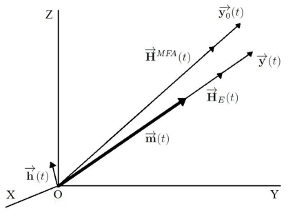
Figure 1: Schematic diagram illustrating the relation between the reduced magnetization m and the vectors $\textbf{H}_{E}$, y, h, $\textbf{H}^{\textit{MFA}}$ and $\textbf{y}_{0}$ at instant $t$ in a non-equilibrium state.

II.2 Final form of the qLLB equation

Eq. (16) is not convenient for numerical modeling or analytical considerations, since at each time step Eq. (15) should be solved to find the variable $\mathbf{y}(t)$ from $\mathbf{m}(t)$. To avoid this issue, we have to make further approximations, for instance, one can use that in ferromagnets the exchange field is strong, $H_{\textrm{E}}\gg h$ in which case $h/H_{E}$ is a small parameter. Thus, in Eq. (16) only the terms linear in this parameter are retained. This assumption is valid both below $T_{c}$ (where always $H_{\textrm{E}}\gg h$) and close to $T_{c}$ where we can use the expansion $H_{\textrm{E}}\simeq(J_{0}/\mu_{\textrm{at}})(m_{e}+\widetilde{\chi}_{\parallel}h)$, where $m_{e}=B_{S}(\beta J_{0}m_{e})$ is the equilibrium magnetization for $h=0$ and

$$\widetilde{\chi}_{\parallel}(T)=\left(\frac{\partial m}{\partial h}\right)_{h\rightarrow 0}$$ (17)

is the reduced linear magnetic susceptibility. Since close to $T_{c}$ the susceptibility is large, $H_{\textrm{E}}\gg h$ for not too strong external magnetic fields. Further simplification in Eq. (16) is obtained using the fact that in stationary dynamic processes $y$ is close to the internal magnetic field direction, ($|y-y_{0}|\ll y$).quantumLLB With these simplifications Eq. (16) is reduced to the qLLB equation in the form

$$\frac{\mathrm{d}\textbf{m}}{\mathrm{d}t} = -\gamma\textbf{m}\times\textbf{H}_{\textrm{eff}}+\gamma\alpha_{\parallel}\frac{\textbf{m}\cdot\textbf{H}_{\textrm{eff}}}{m^{2}}\textbf{m}-\gamma\alpha_{\bot}\frac{\textbf{m}\times(\textbf{m}\times\textbf{H}_{\textrm{eff}})}{m^{2}},$$

where $\textbf{H}_{\textrm{eff}}$ is the effective field given by

$$\textbf{H}_{\textrm{eff}} = \frac{1}{2\widetilde{\chi}_{\parallel}}\left(1-\frac{m^{2}}{m_{e}^{2}}\right)\textbf{m}+\textbf{h}\>\>,\>T<T_{c}.$$ (19)

The longitudinal susceptibility $\widetilde{\chi}_{\parallel}$ can be evaluated in the MFA at $T<T_{c}$ as $\widetilde{\chi}_{\parallel}=\mu_{at}\beta B^{\prime}_{S}/(1-\beta B^{\prime}_{S}J_{0})$ where $B^{\prime}_{S}(x)=dB_{S}/dx$ is evaluated at the equilibrium $B^{\prime}_{S}=B^{\prime}_{S}(\beta J_{0}m_{e})$. The parameters $\alpha_{\parallel}$ and $\alpha_{\perp}$ in Eq. (LABEL:LLBfinalform) are the so-called longitudinal and transverse damping parameters, respectively. In the present article we express them in a form which is suitable for the comparison with the classical LLB equation. Below $T_{c}$ the damping parameters are written as

$$\alpha_{\parallel} = \lambda\frac{2T}{3T_{c}}\frac{2q_{s}}{\sinh\left(2q_{s}\right)}$$ (20)

$$\alpha_{\perp} = \lambda\left[\frac{\tanh(q_{s})}{q_{s}}-\frac{2T}{3T_{c}}\left(1-\frac{K_{1}}{2K_{2}}\right)\right],$$ (21)

where $q_{s}=3T_{c}m_{e}/(2(S+1)T)$ and

$$\lambda=K_{2}\frac{(S+1)}{S}\frac{\mu_{at}}{\gamma k_{B}T}.$$ (22)

In Eq. (LABEL:LLBfinalform) all terms are linear in parameter $h/H_{E}$. Consequently, in Eqs. (20)-(22) the field $\textbf{H}^{\textrm{MFA}}$ in $K_{1}$ and $K_{2}$ can be evaluated at the equilibrium. Note that for $S\rightarrow\infty$ and $K_{1}=K_{2}$, Eqs. (20) and (21) turns to the damping expressions in the classical LLB equation. classicalLLB This allows us to conclude that $\lambda$ represents the intrinsic (Gilbert) damping (coupling to the bath) parameter used in the many-spin atomistic approach. Eq. (22) therefore relates the microscopic damping and the scattering probabilities through Eqs. (7),(8), (12),(13). The temperature dependence of the intrinsic damping is discussed in section III.

Close to $T_{c}$, the effective field used in Eq. (LABEL:LLBfinalform) and given by Eq. (19) is not very convenient for numerical calculations since $m_{e}\rightarrow 0$ and $\widetilde{\chi}_{\parallel}\rightarrow\infty$. To solve this issue we expand the Brillouin function up to the third order in small parameter $x=\beta J_{0}m_{e}$: $B_{S}(x)\simeq ax/3-bx^{3}/45$ and its derivative as $B^{\prime}_{S}(x)\simeq a/3-bx^{2}/15$ where $a=(S+1)/S$ and $b=([2S+1]^{4}-1)/(2S)^{4}$. Thus,

$$m_{e}^{2}\simeq\frac{5A_{s}}{3}\epsilon\quad \quad\widetilde{\chi}_{\parallel}=\frac{\mu_{\textrm{at}}\beta B^{\prime}_{S}}{1-\beta B^{\prime}_{S}J_{0}}\simeq\frac{\mu_{\textrm{at}}}{J_{0}}\frac{1}{2\epsilon},$$ , (23)

where $A_{s}=2(S+1)^{2}/([S+1]^{2}+S^{2})$ and $\epsilon=(T_{c}-T)/T_{c}$ is small close to $T_{c}$. Eq. (19) can be rewritten as

$$\textbf{H}_{\textrm{eff}} = \frac{J_{0}}{\mu_{\textrm{at}}}\left(\epsilon-\frac{3m^{2}}{5A_{s}}\right)\textbf{m}+\textbf{h}\>\>,\>\>|\epsilon|\ll 1.$$ (24)

Above $T_{c}$ we also re-write the effective field in terms of the longitudinal susceptibility at $T>T_{c}$, i.e., $\tilde{\chi}_{\parallel}=\mu_{at}T_{c}/[J_{0}(T-T_{c})]$. This equation is obtained from Eq. (23) and the well-known propertyYeomans of the susceptibility close to $T_{c}$, $2\tilde{\chi}_{\parallel,T<T_{c}}(\epsilon)=\tilde{\chi}_{\parallel,T>T_{c}}(-\epsilon)$. Thus, above $T_{c}$ the effective field is written as

$$\textbf{H}_{\textrm{eff}} = -\frac{1}{\tilde{\chi}_{\parallel}}\left(1+\frac{3T_{c}m^{2}}{5A_{s}(T-T_{c})}\right)\textbf{m}+\textbf{h}\>\>,\>\frac{T_{c}}{T-T_{c}}\gg 1$$

Note that although $\widetilde{\chi}_{\parallel}$ is divergent at $T_{c}$ as corresponds to the second-order phase transition, the internal fields are the same for any $T_{c}-\varepsilon$ and $T_{c}+\varepsilon$ insuring that under the integration of the Eq. (LABEL:LLBfinalform), $\mathbf{m}(t)$ rests continuous through the critical point, as it should be.

On the other hand, in the region just above $T_{c}$, $q_{s}=0$ and $K_{1}\cong K_{2}$ (see section III), so that the damping parameters become approximately the same and equal to

$$\alpha_{\parallel}=\lambda\frac{2T}{3T_{c}},\;\;\alpha_{\perp}=\lambda\frac{2T}{3T_{c}}\left[1+\mathcal{O}(\epsilon)\right],\quad\frac{T_{c}}{T-T_{c}}\gg 1$$ (26)

where the dependence on the spin value $S$ is included implicitly through $\lambda$ [see Eq. (22)]. For $S\rightarrow\infty$ and high temperatures where $K_{1}=K_{2}$ the classical LLB equation above $T_{c}$ is again recovered.

II.3 The qLLB equation for the electron-”impurity” scattering

In this section we derive the qLLB equation for a very simple model for the spin-electron interaction Hamiltonian - the electron-”impurity” scattering model proposed by B. Koopmans et al. in Ref. DallaLonga, and F. Dalla Longa in Ref. Dalla, for the laser induced magnetization dynamics. The model assumes an instantaneous thermalization of the optically excited electrons to the Fermi-Dirac distribution. The Hamiltonian considered here consists of a spin system which weakly interacts with a spinless electron bath and it reads

$$\hat{\mathcal{H}}=\hat{\mathcal{H}}_{s}+\hat{\mathcal{H}}_{e}+\hat{V}_{\textit{s-e}},$$ (27)

where $\hat{\mathcal{H}}_{s}$ is the energy of the spin system, $\hat{\mathcal{H}}_{e}$ stands for the electron bath energy and $\hat{V}_{\textit{s-e}}$ describes the spin-electron interaction energy,

$$\hat{\mathcal{H}}_{s} = -\gamma\mathbf{H}^{\textrm{MFA}}\cdot\hat{\textbf{S}},$$ (28)

$$\hat{\mathcal{H}}_{e} = \sum_{\textbf{k}}\epsilon_{\textbf{k}}\hat{c}_{\textbf{k}}^{\dagger}\hat{c}_{\textbf{k}},$$ (29)

$$\hat{V}_{\textit{s-e}} = -\sum_{\textbf{k},\textbf{k'}}V_{\textbf{k},\textbf{k'}}(\hat{S}^{+}+\hat{S}^{-})\hat{c}_{\textbf{k}}^{\dagger}\hat{c}_{\textbf{k'}}.$$ (30)

Here $\hat{c}^{\dagger}_{\textbf{k}}$ ($\hat{c}_{\textbf{k}}$) is the creation (annihilation) operator which creates (annihilates) an electron with momentum k, $\epsilon_{\textbf{k}}=\hbar^{2}k^{2}/(2m_{el})$, $m_{el}$ is the electron mass, $V_{\textbf{k},\textbf{k'}}$ describes the scattering amplitude. The vector $\mathbf{H}^{\textrm{MFA}}$ is given by Eq. (3). Note that we have chosen for the spin-electron interaction the minimal model that can capture the main features of the physics involved in the magnetization dynamics. In a slightly more sophisticated approach the electron-phonon scattering may be also included, leading to the two-temperature model. Koopmans More rigorous approach, the sp-d model, allows the description of the ultrafast magnetization dynamics in magnetic semiconductorsLukas and ferromagnetic metals.Manchon ; Gridnev

Following the same procedure as in the section II.A, we obtain

$$\frac{d}{dt}\hat{X}^{mn}(t)=i\gamma H^{\textrm{MFA}}(m-n)\hat{X}^{mn}(t)$$ (31)

$$- W_{2}\Big{\{}\frac{1}{2}\left[l^{2}_{m}+l_{n}^{2}+e^{-y_{0}}(l^{2}_{m-1}+l^{2}_{n-1})\right]\hat{X}^{mn}(t)$$

$$- l_{m-1}l_{n-1}\hat{X}^{m-1,n-1}(t)-e^{-y_{0}}l_{m}l_{n}\hat{X}^{m+1,n+1}(t)\Big{\}}$$

where

$$W_{2} = 2\pi\sum_{\textbf{k},\textbf{k'}}|V_{\textbf{k},\textbf{k'}}|^{2}\widetilde{n}_{\textbf{k}}(1-\widetilde{n}_{\textbf{k'}})\delta\left(\gamma H^{\textrm{MFA}}-\frac{\epsilon_{\textbf{k}}-\epsilon_{\textbf{k'}}}{\hbar}\right),$$ (32)

$\widetilde{n}_{\textbf{k}}=[\exp(\beta(\epsilon_{\textbf{k}}-\mu))+1]^{-1}$ is the Fermi-Dirac distribution and $\mu$ is the chemical potential. Comparing Eq. (31) and Eq. (6) we can see that this mechanism leads to the same formal form for the qLLB equation but with $W_{1}=0$. We notice that since $W_{1}=0$ we have $K_{1}=0$, and the damping parameters below $T_{c}$ are given by

$$\alpha_{\parallel} = \lambda\frac{2T}{3T_{c}}\frac{2q_{s}}{\sinh\left(2q_{s}\right)}$$ (33)

$$\alpha_{\perp} = \lambda\left[\frac{\tanh(q_{s})}{q_{s}}-\frac{2T}{3T_{c}}\right].$$ (34)

Differently to the isotropic spin-phonon scattering qLLB equation, considered above, for the electron-”impurity” scattering qLLB equation in the region just above $T_{c}$ the damping parameters are not approximately the same, i.e.,

$$\alpha_{\parallel}=\lambda\frac{2T}{3T_{c}},\;\;\alpha_{\perp}=\lambda\frac{T}{3T_{c}}\left[1+\mathcal{O}(\epsilon)\right],\quad\frac{T_{c}}{T-T_{c}}\gg 1.$$ (35)

Note that this is a consequence of the fact that the model (30) assumes an anisotropic scattering. In the qLLB model with anisotropic phonon’s scattering, defined by $\eta_{z}=\eta_{y}=0$ and $\eta_{x}=2$ we obtain the same result (with a different value of $K_{2}$).

We should point out that the temperature in the qLLB equation for the electron-”impurity” scattering corresponds to the electron bath temperature while for the spin-phonon scattering corresponds to the phonon bath temperature. Therefore, these results validate the coupling of the qLLB equation to the electron bath temperature in the modeling of ultrafast laser induced magnetization dynamics.

II.4 The special case with $S=1/2$.

In the case of $S=1/2$ we can get more simple forms of the qLLB equation. Indeed, in this case $m(t)=B_{1/2}(y(t)/2)=\tanh(y(t)/2)$ and $m_{0}(t)=B_{1/2}(y_{0}(t)/2)=\tanh(y_{0}(t)/2)$. Moreover, Eq. (16) can be further simplified assuming a strong exchange field ($H_{E}\gg h$) which implies

$$\frac{\mathbf{m}\cdot\mathbf{H}^{MFA}}{m\cdot H^{MFA}} = 1+O\left(\left[\frac{h}{H_{E}}\right]^{2}\right),$$ (36)

$$(\mathbf{m}\times\mathbf{H}^{MFA})^{2} = O\left(\left[\frac{h}{H_{E}}\right]^{2}\right),$$ (37)

and using the vectorial relation $\textbf{a}\times(\textbf{b}\times\textbf{c})=\textbf{b}(\textbf{a}\cdot\textbf{c})-\textbf{c}(\textbf{a}\cdot\textbf{b})$, Eq. (16) becomes

$$\frac{\textrm{d}\mathbf{m}}{\textrm{d}t}=-\gamma\mathbf{m}\times\mathbf{h}-(K_{1}+K_{2})\mathbf{m}+\left[2K_{2}+(K_{1}-K_{2})\frac{m}{m_{0}}\right]\mathbf{m}_{0},$$ (38)

where $\mathbf{m}_{0}=\tanh(y_{0}/2)\mathbf{H}^{\textrm{MFA}}/H^{\textrm{MFA}}$ and $K_{1},K_{2}$ can be evaluated at equilibrium. In two special cases: (a) when $K_{1}=K_{2}$ or (b) for longitudinal processes only, i.e. for collinear m, $\textbf{m}_{0}$ and $\mathbf{H}^{\textrm{MFA}}$ this equation can be further simplified. In both cases the Eq. (38) becomes

$$\frac{\textrm{d}\mathbf{m}}{\textrm{d}t}=-\gamma\mathbf{m}\times\mathbf{h}-\frac{\mathbf{m}-\mathbf{m}_{0}}{\tau_{s}},$$ (39)

where $\tau_{s}=1/(2K_{2})$ and the precessional term is zero for the case (b). Eq. (39) in Ref. SCBloch, was called the self-consistent Bloch (SCB) equation.

For the case (b) of a pure longitudinal dynamics the Eq. (38) becomes

$$\frac{\textrm{d}m}{\textrm{d}t}=-\frac{m}{\tau_{s}}\left[1-\frac{\tanh\left(\frac{y_{0}}{2}\right)}{\tanh\left(\frac{y}{2}\right)}\right].$$ (40)

Assuming as before that in dynamical processes the deviations between $y$ and $y_{0}$ are small i.e. $|y-y_{0}|\ll y$ we approximate

$$1-\frac{\tanh\left(\frac{y_{0}}{2}\right)}{\tanh\left(\frac{y}{2}\right)}=\frac{\tanh\left(\frac{y}{2}\right)}{\tanh\left(\frac{y_{0}}{2}\right)}-1+\mathcal{O}([y-y_{0}]^{2}),$$ (41)

and replacing Eq. (41) in Eq. (40) one gets

$$\frac{\textrm{d}m}{\textrm{d}t}=\frac{m}{\tau_{s}}\left[1-m\coth\left(\frac{y_{0}}{2}\right)\right].$$ (42)

We notice that for the case of strong exchange field ($|\textbf{H}_{E}|\gg|\textbf{h}|$) and $S=1/2$ we can write $y_{0}/2\simeq\beta\gamma\ \hbar H_{E}/2=mT_{c}/T$. Eq. (42) is the same as used in the M3TM model,Koopmans in which case ${\tau_{s}}$ is related to concrete Elliott-Yafet scattering mechanism.

III Temperature dependence of the relaxation parameters

The two main parameters which define the properties of the macroscopic magnetization dynamics can be obtained by linearisation of the LLB equation. Namely, they are the longitudinal relaxation time

$$\tau_{\parallel}=\frac{\widetilde{\chi}_{\parallel}}{\gamma\alpha_{\parallel}},$$ (43)

and the transverse relaxation time $\tau_{\bot}$, i.e. the characteristic time taken by the transverse component of magnetization to relax to the effective field $\mathbf{h}$ including the external field and the anisotropy contributions

$$\tau_{\perp}=\frac{m_{e}}{\gamma\,h\alpha_{\perp}}.$$ (44)

The corresponding transverse relaxation term of Eq. (LABEL:LLBfinalform) below $T_{c}$ may be put in the more common form of the macroscopic LLG equation. For this instead of the normalization of magnetisaion to the total spin polarisation, one should use its normalisation to the saturation magnetization value, i.e. $M_{e}(T)$. The resulting equation is the same LLB oneAtxitiaQ but with a different damping parameters, called here $\alpha_{\textrm{LLG}}$. This allows to link the transverse magnetization dynamics described by the LLB equation with the macroscopic (Gilbert-like) temperature-dependent damping

$$\tau_{\perp}^{-1}\propto\alpha_{\textrm{LLG}}=\frac{\alpha_{\perp}}{m_{e}}.$$ (45)

Note that while both $\alpha_{\parallel}$ and $\alpha_{\perp}$ are continuous through $T_{C}$, the parameters $\tau_{\parallel}$ and $\alpha_{\textrm{LLG}}$ diverge at $T_{c}$, corresponding to the critical behavior at the phase transition. Next we consider some limiting cases for these characteristic parameters, for relatively low temperatures and temperatures close to $T_{c}$.

III.1 Longitudinal relaxation time

The longitudinal relaxation time fundamentally depends on the longitudinal susceptibility, $\widetilde{\chi}_{\parallel}$ and the longitudinal damping parameter, $\alpha_{\parallel}$. For the longitudinal susceptibility, using the expansions of the Brillouin function in the corresponding temperature regimes, we obtain

$$\widetilde{\chi}_{||}\cong\frac{\mu_{at}}{k_{B}T_{c}}\begin{cases}\frac{T_{c}}{TS^{2}}e^{-\frac{3T_{c}m_{e}}{T(S+1)}}&\qquad T\ll\min(T_{c},\frac{T_{c}}{S}),\\ \frac{T}{9T_{c}}\left(\frac{S+1}{S}\right)&\qquad\frac{T_{c}}{S}\ll T\ll T_{c},\\ \frac{(S+1)}{6S}\frac{T_{c}}{(T_{c}-T)}&\qquad\frac{T_{c}}{T_{c}-T}\gg 1,\\ \frac{(S+1)}{3S}\frac{T_{c}}{(T-T_{c})}&\qquad\frac{T_{c}}{T-T_{c}}\gg 1.\end{cases}$$ (46)

Note that the region $T\ll\min(T_{c},\frac{T_{c}}{S})$ does not allow the transition to the classical case ($S\rightarrow\infty$). This transition takes place only in the region $T_{c}/S\ll T\ll T_{c}$, the latter condition can be satisfied for $S\gg 1$ only. This means that for a given spin $S\gg 1$ the quantum case becomes approximately the classical one only at temperatures $T\gg T_{c}/S$ (or more exactly $T\gg 3T_{c}m_{e}/2S$), this result is obtained from the analysis of the conditions in which the Brillouin function becomes approximately the Langevin one. Using Eqs. (46) and the asymptotic behavior of $\alpha_{\parallel}$ in the limiting cases, the longitudinal relaxation time in the limiting cases is given by:

$$\tau_{||}\cong\frac{\mu_{at}}{2\gamma\lambda k_{B}T_{c}}\frac{S+1}{S}\begin{cases}\frac{T_{c}}{TS}&\>T\ll\min(T_{c},\frac{T_{c}}{S}),\\ \frac{1}{3}\left[1+\left(\frac{S}{S+1}\right)\frac{T}{T_{c}}\right]&\>\frac{T_{c}}{S}\ll T\ll T_{c},\\ \frac{T_{c}}{2(T_{c}-T)}&\>\frac{T_{c}}{T_{c}-T}\gg 1,\\ \frac{T_{c}}{T-T_{c}}&\>\frac{T_{c}}{T-T_{c}}\gg 1.\end{cases}$$ (47)

Note that our results are in agreement with the well-known relation, proposed by Koopmans et al. Koopmans that the ultrafast demagnetization time scales with the ratio $\mu_{at}/T_{c}$. As we pointed out elsewhere, AtxitiaQ the complete expression involves also the internal coupling to the bath parameter $\lambda$, defined by the scattering rate. The two last lines in Eq. (47) describe the effect of the critical slowing down near the critical temperature. Furthermore, the relaxation time decreases with the increase of the quantum number $S$. Note also that the longitudinal relaxation time is twice larger above $T_{c}$ than below $T_{c}$.

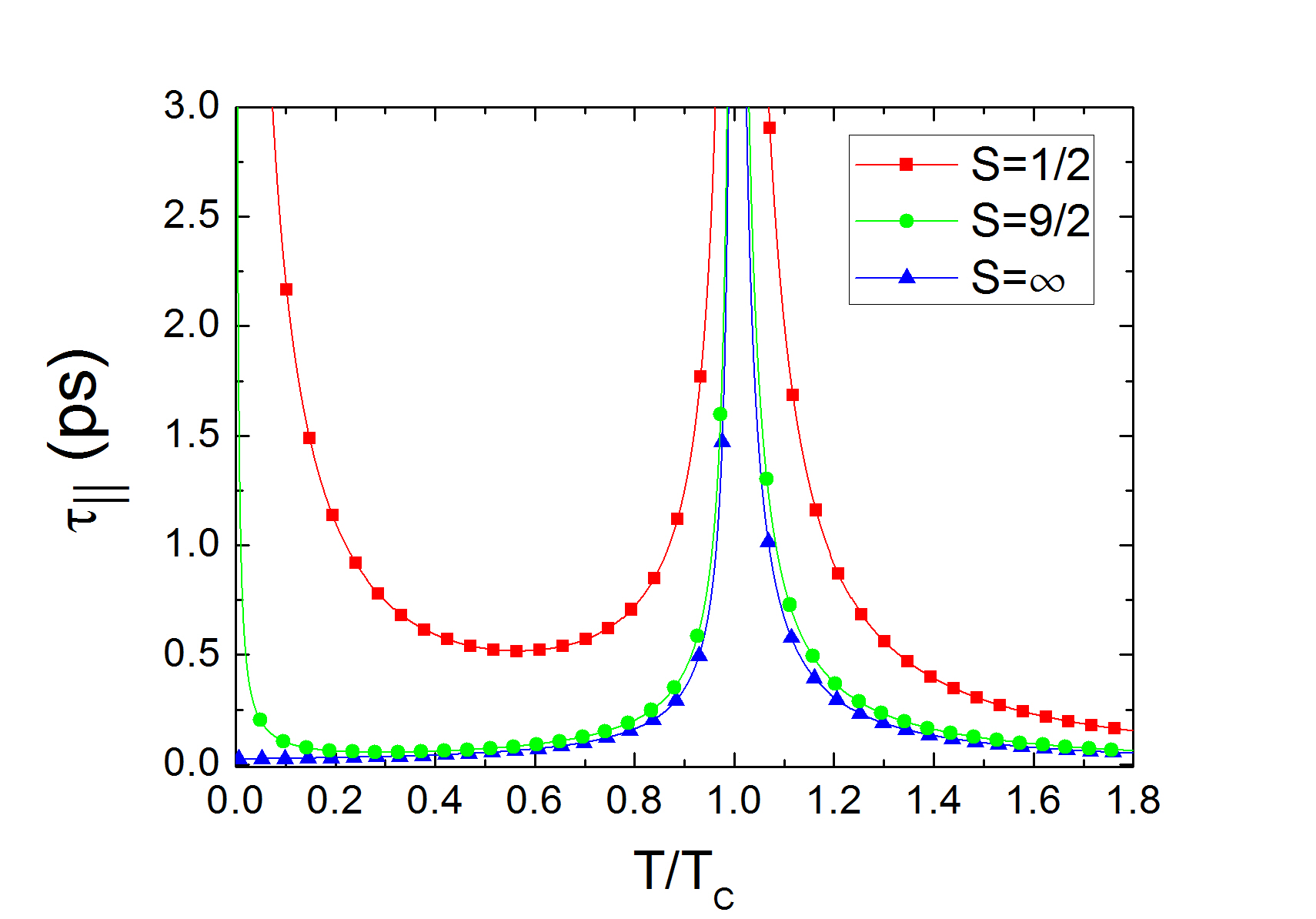
Figure 2: Longitudinal relaxation time (Eq. (43)) versus temperature using constant $\lambda=0.02$, $T_{c}=650\>\textrm{K}$ and $\mu_{at}=0.5\mu_{B}$ in the three spin cases with $S=1/2$, $S=9/2$ and $S=\infty$. The case $S=\infty$ is done by taking the limit $S\rightarrow\infty$ in Eq. (43), which is equivalent to the classical LLB equation.

Normally in the atomistic simulations one uses a constant in temperature coupling to the bath parameter $\lambda=$const. This gives the behaviour for the longitudinal relaxation time that we show in Fig. 2 for the two limiting cases $S=1/2$ and $S=\infty$ and an intermediate case $S=9/2$. In the whole range of parameters the longitudinal relaxation slows down with the decrease of the spin value $S$. For a finite spin number $S$ we observe a divergence of the relaxation time at low temperatures which does not happen for $S=\infty$. The intermediate case $S=9/2$ interpolates between a completely quantum case and a classical case. In this case, all asymptotic behaviors, described by Eqs. (47) are observed, the longitudinal relaxation time diverges at low temperatures (as in the quantum case), is almost constant in the intermediate region (as in the classical case) and again diverges approaching to $T_{c}$.

The divergence of the longitudinal relaxation time at low temperatures seems to be unphysical although it may be attributed to the freezing of the bath degrees of freedom and therefore, impossibility to absorb the energy from the spin system. One should note, however, that taking into account concrete physical mechanisms, the internal damping parameter $\lambda$ becomes temperature-dependent via Eq. (22).

In Fig. 3 we present the longitudinal relaxation time as a function of the temperature in constant applied field for the two limiting cases $S=1/2$ and $S=\infty$. The longitudinal relaxation time was evaluated by direct integration of the qLLB equation with initial conditions $m_{0}-m_{e}=0.1m_{e}$. The longitudinal relaxation time is smaller in the classical case than for the quantum one and, as expected, the maximum is displaced for larger values at larger fields. At $T\approx T_{C}$ the longitudinal relaxation time follows the expression

$$\tau_{||}(H,T=T_{C})=\frac{5A_{S}\mu_{at}}{6\gamma\lambda J_{0}m_{H}^{2}},\;\;m_{H}=\left(\frac{5A_{S}\mu_{at}H}{3J_{0}}\right)^{1/3}$$ (48)

where $m_{H}$ is the field-induced equilibrium magnetisation at $T_{c}$. Therefore, unlike the statement of Ref. SCBloch, , the in-field longitudinal relaxation time, calculated with LLB, does not present any divergence at the Curie temperature.

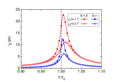
Figure 3: The in-field longitudinal relaxation time calculated via direct integration of the qLLB equation with small deviation from the equilibrium. The following parameters are used $T_{c}=650$ K, $\mu_{\mathrm{at}}=0.5\mu_{B}$, $\lambda=0.02$ and zero anisotropy constant. $\mu_{0}$ is the permeability of free space.

III.2 Transverse LLG-like damping parameter

For the transverse damping we obtain the following limits

$$\alpha_{LLG}\cong\lambda\begin{cases}\frac{T}{3T_{c}}\left(2S+\frac{K_{1}}{K_{2}}\right)&\qquad T\ll\min(T_{c},\frac{T_{c}}{S}),\\ \left[1-\frac{1}{2S}-\frac{T}{3T_{C}}\left(1-\frac{K_{1}}{K_{2}}\right)\right]&\qquad\frac{T_{c}}{S}\ll T\ll T_{c},\\ \left(1+\frac{K_{1}}{K_{2}}\right)\sqrt{\frac{T_{c}}{15A_{S}(T_{c}-T)}}&\qquad\frac{T_{c}}{T_{c}-T}\gg 1.\end{cases}$$ (49)

The temperature dependence of the LLG damping parameter for a constant value of $\lambda$ and $K_{1}=K_{2}$ is presented in Fig. 4 for the two limiting cases $S=1/2$ and $S=\infty$ and the intermediate case $S=9/2$. In this case the transverse damping parameter tends to a constant value in the classical case and to a zero value in the quantum case. The transverse relaxation also becomes faster with the increase of the spin number. For simplicity, we have used $\lambda=$const and $K_{1}=K_{2}$ in Fig. 4 but, as we have seen before, the quantities $K_{1}$, $K_{2}$ and $\lambda$ depend on the particular scattering mechanism. Next we study the same limits but taking into account the scattering mechanisms, considered here.

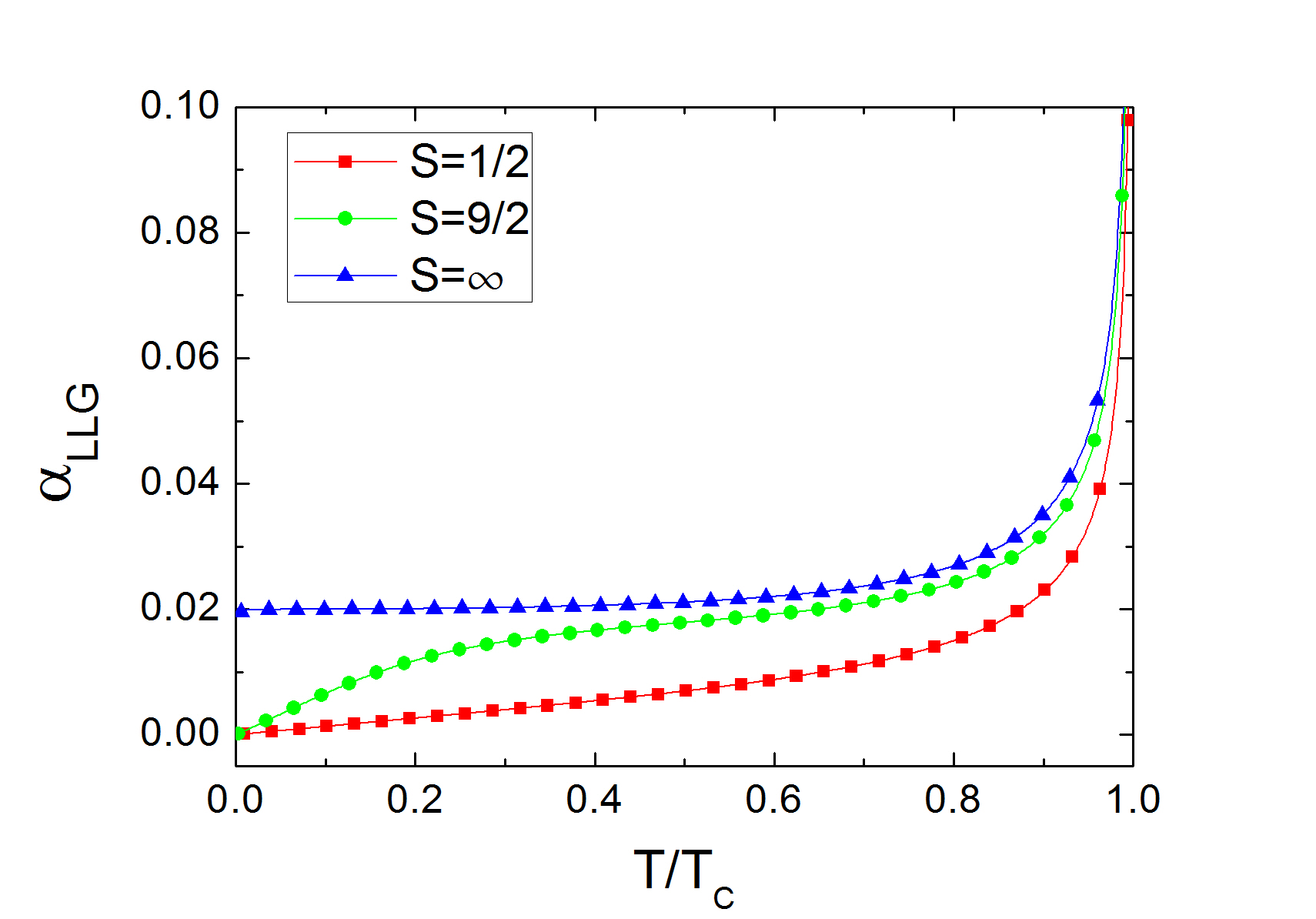
Figure 4: LLG damping (Eq. (45)) versus temperature using $K_{1}=K_{2}$, constant $\lambda=0.02$, $T_{c}=650\>\textrm{K}$ and $\mu_{at}=0.5\mu_{B}$ for the three spin cases $S=1/2$, $S=9/2$ and $S=\infty$. The case $S=\infty$ is done by taking the limit $S\rightarrow\infty$ in Eq. (45), which is equivalent to the classical case.

III.3 Relaxation parameters with temperature-dependent internal scattering mechanisms

III.3.1 Scattering via phonons

For the spin-phonon scattering we can evaluate $W_{1}$ and $W_{2}$ in Eqs. (7), (8) using spin-phonon couplings of the typeGaranin4

$$V_{q}=\frac{\theta_{1}}{v}\sqrt{\frac{\omega_{q}}{M}}\quad,\quad V_{pq}=\theta_{2}\frac{\sqrt{\omega_{p}\omega_{q}}}{Mv^{2}}$$ (50)

where $\theta_{1}$ and $\theta_{2}$ are constants, $M$ is the unit cell mass and $v$ is the speed of sound in the material. The evaluation of $K_{1}$ and $K_{2}$ in Eqs. (12), (13) gives the following result

$$K_{1}\ll K_{2}\simeq\frac{\theta_{1}^{2}\Omega(\gamma H^{\textrm{MFA}})^{3}}{4\pi Mv^{5}}\quad \quad k_{B}T\ll\hbar\gamma H^{\textrm{MFA}}$$ , (51)

$$K_{1}\simeq K_{2}\simeq\left[\frac{\theta_{2}^{2}\Omega^{2}k_{B}^{7}T_{D}^{5}}{20\pi^{3}M^{2}v^{10}\hbar^{7}}\right]T^{2}\quad \quad\hbar\gamma H^{\textrm{MFA}}\ll k_{B}T_{D}\ll k_{B}T$$ ,

where $T_{D}$ is the Debye temperature and $\Omega$ is the unit-cell volume. Using Eqs. (51), (III.3.1) in Eq. (22) we obtain

$$\lambda_{ph}\propto\begin{cases}\frac{1}{T}&\qquad k_{B}T\ll\hbar\gamma H^{\textrm{MFA}},\\ T&\qquad\hbar\gamma H^{\textrm{MFA}}\ll k_{B}T_{D}\ll k_{B}T.\end{cases}$$ (53)

Therefore, if we take into account the temperature dependence of $K_{1}$, $K_{2}$ and $\lambda$ for the phonon scattering mechanism in Eqs. (47) and (49) we obtain

$$\tau_{||,ph}\propto\begin{cases}\textrm{const}&\quad T\ll\min(T_{c},\frac{T_{c}}{S})\>,\>k_{B}T\ll\hbar\gamma H^{\textrm{MFA}}\\ T&\quad\frac{T_{c}}{S}\ll T\ll T_{c}\>,\>k_{B}T\ll\hbar\gamma H^{\textrm{MFA}}\\ \frac{1}{T|T_{c}-T|}&\quad\frac{|T_{c}-T|}{T_{c}}\ll 1\>,\>\hbar\gamma H^{\textrm{MFA}}\ll k_{B}T_{D}\ll k_{B}T,\end{cases}$$ (54)

and

$$\alpha_{LLG,ph}\propto\begin{cases}\textrm{const}&\quad T\ll\min(T_{c},\frac{T_{c}}{S})\>,\>k_{B}T\ll\hbar\gamma H^{\textrm{MFA}},\\ \frac{1}{T}&\quad\frac{T_{c}}{S}\ll T\ll T_{c}\>,\>k_{B}T\ll\hbar\gamma H^{\textrm{MFA}}\\ \frac{T}{\sqrt{T_{c}-T}}&\quad\frac{T_{c}}{T_{c}-T}\gg 1\>,\>\hbar\gamma H^{\textrm{MFA}}\ll k_{B}T_{D}\ll k_{B}T.\end{cases}$$ (55)

We observe that in the case of a pure phonon mechanism, the longitudinal relaxation time does not diverge at low temperatures. On the other hand, at elevated temperatures the longitudinal magnetization dynamics is slowed down, since close to $T_{c}$ it is dominated by the divergence of $\widetilde{\chi}_{\|}$ [see Eq. (46)] rather than by the longitudinal damping parameter, $\alpha_{\parallel}\propto T+\mathcal{O}({\epsilon})$. However, since $\tau^{-1}_{\bot}\propto\alpha_{\textrm{LLG}}$ we see that at high temperature the transverse magnetization dynamics becomes faster as the temperature gets closer to $T_{c}$.

III.3.2 Scattering via electrons

For the electron-”impurity” scattering we have found before that $K_{1}=0$, but we should still evaluate $K_{2}$. For this task, we calculate the quantity $W_{2}$ given by Eq. (32) assuming that $|V_{\textbf{k},\textbf{k'}}|^{2}=\mathcal{V}=\textrm{const}$ and constant density of states around the Fermi level $D(\epsilon_{F})$ (as in Refs. DallaLonga, and Dalla, ). For this case, we obtain

$$W_{2} = \frac{\pi\mathcal{V}\hbar D(\epsilon_{F})^{2}}{2}\left[\frac{\hbar\gamma H^{\textrm{MFA}}}{1-e^{-\beta\hbar\gamma H^{\textrm{MFA}}}}\right],$$ (56)

where $\epsilon_{F}$ is the Fermi energy,

$$D(E)=\frac{\Omega}{2\pi^{2}}\left(\frac{2m_{el}}{\hbar^{2}}\right)^{\frac{3}{2}}\sqrt{E}$$ (57)

is the density of states for a free electron gas (taking into account the spin degeneracy) and $\Omega$ is the system volume. Replacing Eq. (56) in Eq. (13), the following limiting cases for $K_{2}$ are obtained:

$$K_{2} = \frac{\pi\mathcal{V}\hbar^{2}D(\epsilon_{F})^{2}\gamma H^{\textrm{MFA}}}{4}\begin{cases}1&\qquad k_{B}T\ll\hbar\gamma H^{\textrm{MFA}}\\ \frac{2k_{B}T}{\hbar\gamma H^{\textrm{MFA}}}&\qquad\hbar\gamma H^{\textrm{MFA}}\ll k_{B}T\\ \end{cases},$$

and then from Eq. (22) we obtain

$$\lambda_{el}\propto\begin{cases}\frac{1}{T}&\qquad k_{B}T\ll\hbar\gamma H^{\textrm{MFA}},\\ \textrm{const}&\qquad\hbar\gamma H^{\textrm{MFA}}\ll k_{B}T.\end{cases}$$ (58)

We observe that at low temperatures ($k_{B}T\ll\hbar\gamma H^{\textrm{MFA}}$) $\lambda$ has the same temperature dependence as in the phonon scattering case, so that in this temperature regime we obtain the same results for $\tau_{||}$ and $\alpha_{LLG}$ as in Eqs. (54) and (55). However, at high temperatures ($\hbar\gamma H^{\textrm{MFA}}\ll k_{B}T$) we have $\lambda_{el}=\textrm{const}$, which validates the use of the constant $\lambda$ value in the modeling of the laser-induced magnetization dynamics, where the main mechanism is electronic and the temperatures are high. In this high temperature regime $\tau_{||}$ and $\alpha_{LLG}$ have the following temperature dependencies

$$\tau_{||,el}\propto\frac{1}{|T_{c}-T|}\qquad\frac{|T_{c}-T|}{T_{c}}\ll 1\>,\>\hbar\gamma H^{\textrm{MFA}}\ll k_{B}T,$$ (59)

and

$$\alpha_{LLG,el}\propto\frac{1}{\sqrt{T_{c}-T}}\qquad\frac{T_{c}}{T_{c}-T}\gg 1\>,\>\hbar\gamma H^{\textrm{MFA}}\ll k_{B}T.$$ (60)

In this case, we also obtain a critical behavior of $\tau_{||}$ and $\alpha_{LLG}$ close to $T_{c}$.

IV Numerical comparison between classical and quantum cases

In this section we compare the qLLB equation for $S=1/2$ and its classical limit ($S\gg 1$). We use the qLLB equation given by Eq. (LABEL:LLBfinalform) for the isotropic phonon scattering mechanism and the high temperature case ($K_{1}=K_{2}$). We note that for a proper comparison between classical and quantum cases, one should take the same magnetic moment $\mu_{\textrm{at}}$ and Curie temperature $T_{c}$ (normally obtained from the experimental measurements) and not vary them with the spin number $S$. In the opposite case the magnetic moment would increase with $S$ and the Curie temperature decrease and the classical modeling results will not be recovered.

In our simulations we set $\gamma=1.76\times 10^{11}$ rad s^-1 T^-1, $T_{c}=650$ K, $\mu_{\mathrm{at}}=0.5\mu_{B}$ and $\lambda=0.02$ and zero anisotropy constant. Note that in order to be consistent with the comparison of the SCB with $S=1/2$ (indistinguishable from the qLLB with $S=1/2$) and the classical LLB equation, presented in Ref. SCBloch2, , we choose similar parameters and situations. In Fig. 5 we present the dynamics of $m_{z}$ component for $S=1/2,\infty$ and for different temperatures where the initial magnetization is set to $\textbf{m}=(0.05,0,0.2)$ and the external applied field is $\mu_{0}H_{z}=-1\textrm{T}$, where $\mu_{0}$ is the permeability of free space. The initial response is slower for $S=1/2$ than for $S=\infty$ in agreement with the behavior of the longitudinal relaxation time, presented in Fig. 2. Note the variety of different functional responses and that for the two cases below $T_{c}$ they cannot be represented as a one-exponential relaxation due to the nonlinearity of the LLB equation, prominent for $T$ close to $T_{c}$.

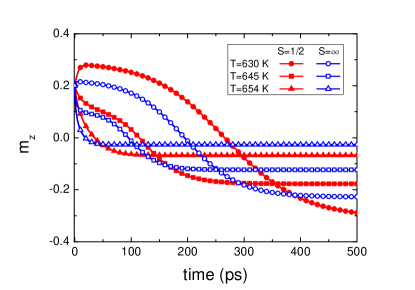
Figure 5: The dynamics of $m_{z}$ component for the longitudinal plus transverse dynamics at $630$ K, $645$ K and $654$ K for $S=1/2,\infty$ where the initial magnetization is $\textbf{m}=(0.05,0,0.2)$ and the applied field is $\mu_{0}H_{z}=-1\textrm{T}$.

In Fig. 6 we present the relaxation of $m_{z}$ at $T=649$ K, with and without an external field ($\mu_{0}H_{z}=-1\textrm{T}$) where the initial magnetization is set to $\textbf{m}=(0.05,0,0.2)$. We use the qLLB equation for $S=1/2$ and $S=\infty$ for comparison. Note that again the dynamics is faster for $S=\infty$ than for $S=1/2$. Since the qLLB and the SCB equations with $S=1/2$ are the same, we conclude that the classical LLB equation gives a faster relaxation than the SCB equation, contrarily to the results presented in Ref. SCBloch2, .

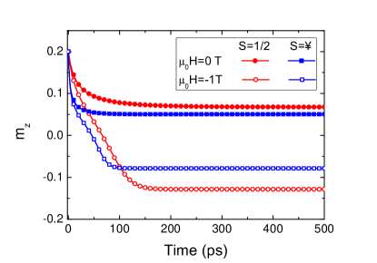
Figure 6: The dynamics of $m_{z}$ component at $T=649$ K without and with external field $\mu_{0}H_{z}=-1\textrm{T}$ for $S=1/2,\infty$ where the initial magnetization is $\textbf{m}=(0.05,0,0.2)$.

Similar to Ref. SCBloch2, we define the reversal time as time elapsed between the initial state and the instant of time at which the magnetization begins to reverse its direction, i.e. crosses $m_{z}=0$ point. In Fig. 7 we present the reversal time versus temperature for $S=1/2,\infty$ and for two different initial conditions: (i) pure longitudinal dynamics where the initial magnetization is set to $\textbf{m}=(0,0,0.2)$ and (ii) longitudinal plus transverse dynamics where the initial magnetization is set to $\textbf{m}=(0.05,0,0.2)$. We observe that the reversal time (for both the quantum and the classical case) does not present any discontinuity across the Curie temperature and is smaller for $S=\infty$ than for $S=1/2$, in contradiction to the results presented in Ref. SCBloch2, where the SCB and the classical LLB equation were compared. As was pointed out in several previous publications, GaraninChubykalo ; KazantsevaEPL ; BarkerAPL slightly below $T_{c}$ the magnetization reversal becomes linear, i.e. occurs by a pure change of the magnetization magnitude. This path becomes not energetically favorable with the decrease of the temperature, the reversal path becomes elliptical and then completely precessional.

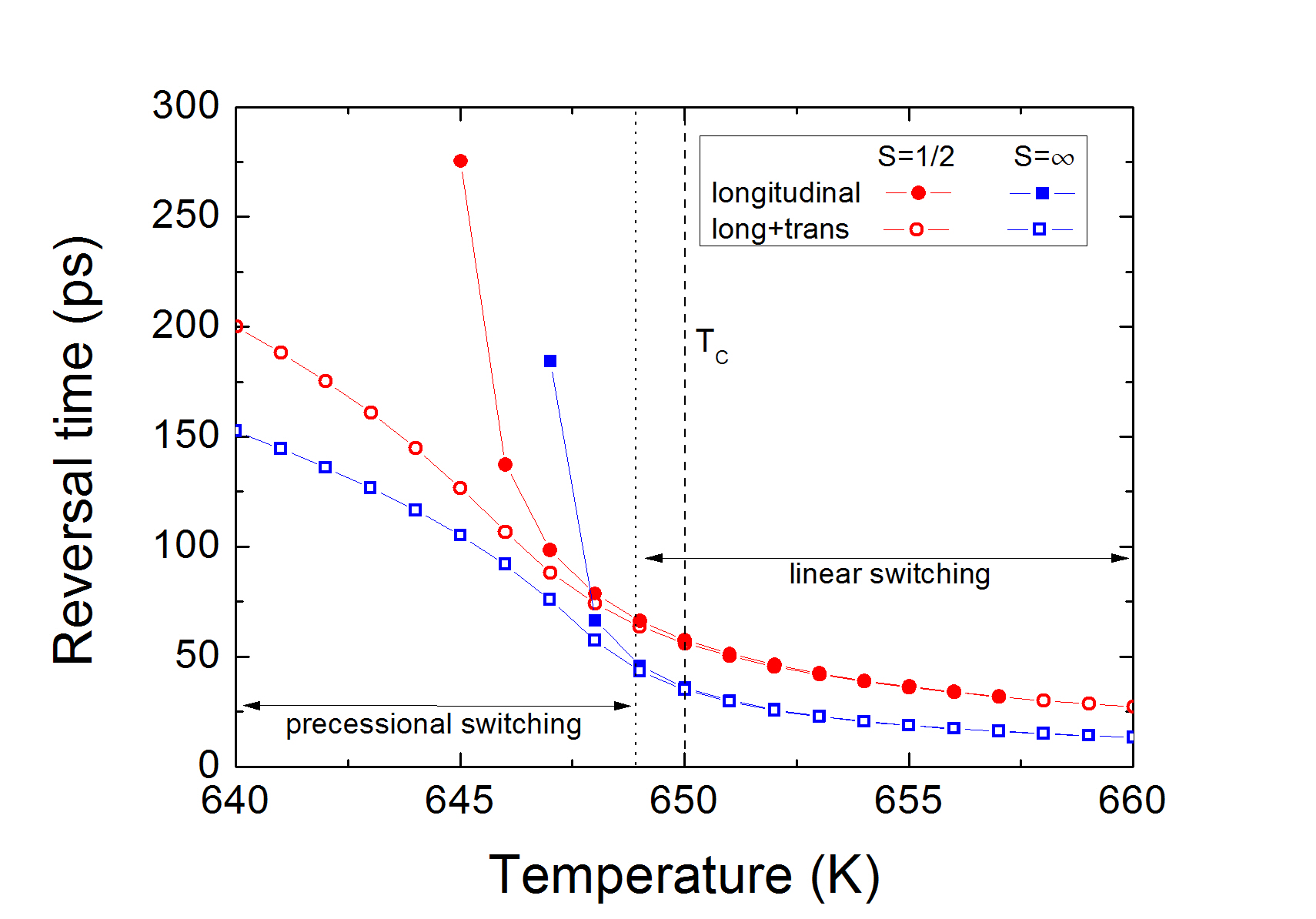
Figure 7: Reversal time versus temperature for $S=1/2,\infty$ and $S=\infty$. In the pure longitudinal dynamics the initial magnetization is set to $\textbf{m}=(0,0,0.2)$ and in the longitudinal plus transverse dynamics the initial magnetization is set to $\textbf{m}=(0.05,0,0.2)$.

V Conclusions

We have presented the derivation of the qLLB equation for two simple scattering mechanisms: based on the phonon and the electron-impurity spin-dependent scattering. While the spin-phonon interaction has been historically thought as the main contribution to the damping mechanism (for transverse magnetization dynamics), for the ultrafast laser induced magnetization dynamics the electron mechanism is considered to be the most important contribution. At the same time, the induction of the ultrafast magnetization dynamics via acoustic excitation is becoming increasingly important so that the importance of the phonon-mediated mechanism is still relevant for femtomagnetism. Although in the present work we have only considered the simplest form for the spin-phonon and -electron interaction Hamiltonian, the derivation could be generalized to more complex situations. The form of equation (LABEL:LLBfinalform) is sufficiently general and at present can be used for modeling of most of the experimental cases, understanding that the parameter $\lambda$ contains all necessary scattering mechanisms and can be extracted from experimental measurements as it was done before, AtxitiaNi ; AtxitiaQ ; Sultan ; Koopmans similar to the Gilbert damping parameter in standard micromagnetic modeling. Importantly, the recently proposed self-consistent Bloch equation SCBloch ; SCBloch2 and the M3TM model are contained in the qLLB model. Koopmans

The derivation involves two important approximations: the Markov and the secular. Their validity could be questionable for the ultrafast processes and in the future these approximations should be investigated. At the same time, our comparisons with experiments for Ni,AtxitiaNi GdSultan and FePtFePt have shown a very good agreement.

The derivation has allowed us to relate the classical internal coupling to the bath parameter $\lambda$, used in the atomistic spin model simulations, to the scattering probabilities which could be evaluated on the basis of the ab-initio electronic structure calculations, providing the route to a better scheme of the multi-scale modeling of magnetic materials. The temperature dependence of $\lambda$ will depend on the nature of the concrete scattering mechanism. In the present paper we have shown that this parameter is temperature dependent. At the same time, the use of the temperature-independent microscopic damping (coupling to the bath parameter) for laser-induced magnetization dynamics, as it is normally done in the atomistic simulations, is probably reasonable. Our results also include the temperature dependence of macroscopic relaxation parameters: the longitudinal relaxation and the LLG-like transverse damping. We have shown that both transverse and longitudinal relaxation are faster in the classical case than in the quantum one.

The comparison between the classical and the quantum LLB equations has been done in the conditions of the same magnetic moment and the Curie temperature, as corresponds to the spirit of the classical atomistic modeling. Unlike the statement appearing in Ref. SCBloch2, , the magnetization is continuous when going through $T_{c}$, the same happens with the reversal time. In the considered case in this work, the reversal time is smaller in the classical case than in the quantum one, although our investigation shows that this result depends on the system parameters.

Our results contribute to a construction of correct multi-scale/micromagnetic approach for the modeling of high-temperature and/or short timescale magnetization dynamics. The obtained micromagnetic approach can be used for modeling of large structures, such as dots and stripes up to micron-sizes, under the conditions where the use of the LLB equation is necessary.

References

- (1) O. Chubykalo-Fesenko, U. Nowak, R. W. Chantrell, and D. Garanin, Phys. Rev. B 74, 094436 (2006).
- (2) K. M. Lebecki, D. Hinzke, U. Nowak, and O. Chubykalo-Fesenko, Phys. Rev. B 86, 094409 (2012).
- (3) T. McDaniel, J. Appl. Phys. 112, 013914 (2012).
- (4) U. Kilic, G. Finocchio, T. Hauet, S. H. Florez, G. Aktas, and O. Ozatay Appl. Phys. Lett. 101, 252407 (2012).
- (5) C. Schieback, D. Hinzke, M. Klaüi, U. Nowak, and P. Nielaba, Phys. Rev. B 80, 214403 (2009).
- (6) D. Hinzke and U. Nowak, Phys. Rev. Lett. 107, 027205 (2011).
- (7) U. Atxitia, O. Chubykalo-Fesenko, J. Walowski, A. Mann and M. Münzenberg, Phys. Rev. B 81, 174401 (2010).
- (8) K. Vahaplar, A. M. Kalashnikova, A. V. Kimel, D. Hinzke, U. Nowak, R. Chantrell, A. Tsukamoto, A. Itoh, A. Kirilyuk, and Th. Rasing, Phys. Rev. Lett. 103, 117201 (2009).
- (9) A. Kirilyuk, A. Kimel and Th. Rasing, Rev. Mod. Phys. 82, 2731 (2010).
- (10) T. A. Ostler, J. Barker, R. F. L. Evans, R. W. Chantrell, U. Atxitia, O. Chubykalo-Fesenko, S. El Moussaoui, L. Le Guyader, E. Mengotti, L. J. Heyderman, F. Nolting, A. Tsukamoto, A. Itoh, D. Afanasiev, B. A. Ivanov, A. M. Kalashnikova, K. Vahaplar, J. Mentink, A. Kirilyuk, Th. Rasing, and A. V. Kimel, Nature Commun. 3, 666 (2012).
- (11) U. Atxitia and O. Chubykalo-Fesenko, Phys. Rev. B 84, 144414 (2011).
- (12) D. A. Garanin, Physica A 172, 470 (1991).
- (13) U. Atxitia, P. Nieves, and O. Chubykalo-Fesenko, Phys. Rev. B 86, 104414 (2012).
- (14) D. A. Garanin, Phys. Rev. B , 3050 (1997).
- (15) N. Kazantseva, D. Hinzke, U. Nowak, R. W. Chantrell, U. Atxitia, and O. Chubykalo-Fesenko, Phys. Rev. B 77, 184428 (2008).
- (16) B. D. Cullity, Introduction to magnetic materials, Addison- Wesley Publishing Co, 1972.
- (17) I. Radu, K. Vahaplar, C. Stamm, T. Kachel, N. Pontius, H. A. Dürr, T. A. Ostler, J. Barker, R. F. L. Evans, R. W. Chantrell, A. Tsukamoto, A. Itoh, A. Kirilyuk, Th. Rasing, and A. V. Kimel, Nature 472, 205 (2011).
- (18) M. Sultan, U. Atxitia, A. Melnikov, O. Chubykalo-Fesenko, and U. Bovensiepen, Phys. Rev. B , 184407 (2012).
- (19) B. Koopmans, G. Malinowski, F. Dalla Longa, D. Steiauf, M. Faehnle, T. Roth, M. Cinchetti, and M. Aeschlimann, Nature Mater. 9, 259 (2010).
- (20) A. J. Schellekens and B. Koopmans, Phys. Rev. Lett. 110, 217204 (2013).
- (21) B. Y. Mueller, A. Baral, S. Vollmar, M. Cinchetti, M. Aeschlimann, H. C. Schneider, and B. Rethfeld, Phys. Rev. Lett. 111, 167204 (2013).
- (22) L. Xu and S. Zhang, Physica E , 72 (2012).
- (23) R. Bastardis, U. Atxitia, O. Chubykalo-Fesenko and H. Kachkachi, Phys. Rev. B , 094415 (2012).
- (24) A. V. Scherbakov, A. S. Salasyuk, A. V. Akimov, X. Liu, M. Bombeck, C. Brüggemann, D. R. Yakovlev, V. F. Sapega, J. K. Furdyna and M. Bayer, Phys. Rev. Lett. , 117204 (2010).
- (25) J. W. Kim, M. Vomir and J. Y. Bigot, Phys. Rev. Lett. , 166601 (2012).
- (26) D. A. Garanin, Phys. Rev. E , 2569 (1997).
- (27) K. Blum, Density Matrix Theory and Applications (Plenum Press, New York, London, 1981).
- (28) D. A. Garanin, Advances in Chemical Physics, , 213 (2012).
- (29) H. P. Breuer and F. Petruccione, The theory of quantum open systems (Oxford University Press, New York, 2002).
- (30) J. Olšina and T. Mančal, J. Mol. Model , 1765 (2010).
- (31) U. Atxitia, O. Chubykalo-Fesenko, R. W. Chantrell, U. Nowak, and A. Rebei, Phys. Rev. Lett. 102, 057203 (2009).
- (32) D. A. Garanin, V. V. Ishtchenko, and L. V. Panina, Teor. Mat. Fiz. , 169 (1990).
- (33) D. A. Garanin and O. Chubykalo-Fesenko, Phys. Rev. B 70, 212409 (2004).
- (34) D. A. Garanin and E. M. Chudnovsky, Phys. Rev. B , 11102 (1997).
- (35) C. J. Yeomans, Statistical mechanics of phase transitions, Oxford University Press, Oxford, UK, (1995) 126.
- (36) B. Koopmans, J. J. M. Ruigrok, F. Dalla Longa, and W. J. M. de Jonge, Phys. Rev. Lett. 95, 267207 (2005).
- (37) F. Dalla Longa, Laser induced magnetization dynamics -an ultrafast journey among spins and light pulses, PhD thesis, Eindhoven University of Technology, Eindhoven, The Netherlands (2008).
- (38) L. Cywiński and L. J. Sham, Phys. Rev. B , 045205 (2007).
- (39) A. Manchon, Q. Li, L. Xu and S. Zhang, Phys. Rev. B , 064408 (2012).
- (40) V. N. Gridnev, Phys. Rev. B , 014405 (2013).
- (41) L. Xu and S. Zhang, J. Appl. Phys. , 163911 (2013).
- (42) N. Kazantseva, D. Hinzke, R. W. Chantrell and U. Nowak, EPL, , 27006 (2009).
- (43) J. Barker, R. F. L. Evans, R. W. Chantrell, D. Hinzke, and U. Nowak, Appl. Phys. Lett. , 192504 (2010).
- (44) J. Mendil, P. Nieves, O. Chubykalo-Fesenko, J. Walowski, T. Santos, S. Pisana, and M. Münzenberg, Sci. Rep. , 3980 (2014).