Automated detection of coherent Lagrangian vortices in two-dimensional unsteady flows

Abstract

Coherent boundaries of Lagrangian vortices in fluid flows have recently been identified as closed orbits of line fields associated with the Cauchy–Green strain tensor. Here we develop a fully automated procedure for the detection of such closed orbits in large-scale velocity data sets. We illustrate the power of our method on ocean surface velocities derived from satellite altimetry.

Keywords: Coherent Lagrangian vortices, Transport, Index theory, Line fields, Closed orbit detection, Ocean surface flows.

1 Introduction

Lagrangian coherent structures (LCS) are exceptional material surfaces that act as cores of observed tracer patterns in fluid flows (see [22] and [23] for reviews). For oceanic flows, the tracers of interest include salinity, temperature, contaminants, nutrients and plankton—quantities that play an important role in the ecosystem and even in climate. Fluxes of these quantities are typically dominated by advective transport over diffusion.

An important component of advective transport in the ocean is governed by mesoscale eddies, i.e., vortices of $100$–$200$ km in diameter. While eddies also stir and mix surrounding water masses by their swirling motion, here we focus on eddies that trap and carry fluid in a coherent manner. Eddies of this kind include the Agulhas rings of the Southern Ocean. They are known to transport massive quantities of warm and salty water from the Indian Ocean into the Atlantic Ocean [6]. Current limitations on computational power prevent that climate models resolve mesoscale eddies in their flow field. Since the effect of mesoscale eddies on the global circulation is significant [36], the correct parameterization of eddy transport is crucial for the reliability of these models. As a consequence, there is a rising interest in systematic and accurate eddy detection and census in large global data sets, as well as in quantifying the average transport of trapped fluid by all eddies in a given region [9, 38, 25].

This quantification requires (i) a rigorous method that provides specific coherent eddy boundaries, and (ii) a robust numerical implementation of the method on large velocity data sets.

A number of vortex definitions have been proposed in the literature, [15, 37], most of which are of Eulerian type, i.e., use information from the instantaneous velocity field. Typical global eddy studies [5, 9, 38, 25] are based on such Eulerian approaches. Evolving eddy boundaries obtained from Eulerian approaches, however, do not encircle and transport the same body of water coherently [17, 37]. Instead, fluid initialized within an instantaneous Eulerian eddy boundary will generally stretch, fold and filament significantly. Yet only coherently transported scalars resist erosion by diffusion in a way that a sharp signature in the tracer field is maintained. All this suggests that coherent eddy transport should ideally be analysed via Lagrangian methods that take into account the evolution of trajectories in the flow, such as, e.g., [27, 1, 19, 28, 31, 26]. Notably, however, none of these methods focuses on the detection of vortices and none provides an algorithm to extract exact eddy boundaries in unsteady velocity fields.

Only recently have mathematical approaches emerged for the detection of coherent Lagrangian vortices. These include the geometric approach [15, 17] and the set-oriented approach [14, 12, 13]. Here, we follow the geometric approach to coherent Lagrangian vortices, which defines a coherent material vortex boundary as a closed stationary curve of the averaged material strain [17]. All solutions of this variational problem turn out to be closed material curves that stretch uniformly. Such curves are practically found as closed orbits of appropriate planar line fields [17].

In contrast to vector fields, line fields are special vector bundles over the plane. In their definition, only a one-dimensional subspace (line) is specified at each point, as opposed to a vector at each point. The importance of line field singularities in Lagrangian eddy detection has been recognized in [17], but has remained only partially exploited. Here, we point out a topological rule that enables a fully automated detection of coherent Lagrangian vortex boundaries based on line field singularities. This in turn makes automated Lagrangian eddy detection feasible for large ocean regions.

Based on the geometric approach, coherent Lagrangian vortices have so far been identified in oceanic data sets [3, 17], in a direct numerical simulation of the two-dimensional Navier–Stokes equations [11], in a smooth area-preserving map [16], in a kinematic model of an oceanic jet in [16], and in a model of a double gyre flow [21]. With the exception of [17], however, these studies did not utilize the topology of line field singularities. Furthermore, none of them offered an automated procedure for Lagrangian vortex detection.

The orbit structure of line fields has already received considerable attention in the scientific visualization community (see [7, 33] for reviews). The problem of closed orbit detection has been posed in [7, Section 5.2.3], and was considered by [34], building on [35]. In that approach, numerical line field integration is used to identify cell chains that may contain a closed orbit. Then, the conditions of the Poincaré–Bendixson theorem are verified to conclude the existence of a closed orbit for the line field. This approach, however, does not offer a systematic way to search for closed orbits in large data sets arising in geophysical applications.

This paper is organized as follows. In Section 2, we recall the index theory of planar vector fields. In Section 3, we review available results on indices for planar line fields, and deduce a topological rule for generic singularities inside closed orbits of such fields. Next, in Section 4, we present an algorithm for the automated detection of closed line field orbits. We then discuss related numerical results on ocean data, before presenting our concluding remarks in Section 5.

2 Index theory for planar vector fields

Here, we recall the definition and properties of the index of a planar vector field [20]. We denote the unit circle of the plane by $\mathcal{S}^{1}$, parametrized by the mapping $(\cos 2\pi s,\sin 2\pi s)\in\mathcal{S}^{1}\subset\mathds{R}^{2}$, $s\in\left[0,1\right]$. In our notation, we do not distinguish between a curve $\gamma\colon[a,b]\to\mathds{R}^{2}$ as a function and its image as a subset of $\mathds{R}^{2}$.

Definition 1 (Index of a vector field).

For a continuous, piecewise differentiable planar vector field $\mathbf{v}\colon D\subseteq\mathds{R}^{2}\to\mathds{R}^{2}$ and a simple closed curve $\gamma\colon\mathcal{S}^{1}\to\mathds{R}^{2}$, let $\theta\colon\left[0,1\right]\to\mathds{R}$ be a continuous function such that $\theta(s)$ is the angle between the $x$-axis and $\mathbf{v}(\gamma(s))$. Then, the index (or winding number) of  $\mathbf{v}$ along $\gamma$ is defined as

$$\operatorname{ind}_{\gamma}(\mathbf{v})\coloneqq\frac{1}{2\pi}\left(\theta(1)-\theta(0)\right),$$

i.e., the number of turns of $\mathbf{v}$ during one anticlockwise revolution along $\gamma$. Clearly, $\theta$ is well-defined only if there is no critical point of $\mathbf{v}$ along $\gamma$, i.e., no point at which $\mathbf{v}$ vanishes.

The index defined in Definition 1 has two important properties [24]:

1. Decomposition property:

   $$\operatorname{ind}_{\gamma}(\mathbf{v})=\operatorname{ind}_{\gamma_{1}}\left(\mathbf{v}\right)+\operatorname{ind}_{\gamma_{2}}\left(\mathbf{v}\right),$$

   whenever $\gamma=\gamma_{1}\cup\gamma_{2}\setminus(\gamma_{1}\cap\gamma_{2})$, and $\operatorname{ind}_{\gamma_{i}}\left(\mathbf{v}\right)$ are well-defined.

2. Homotopy invariance:

   $$\operatorname{ind}_{\gamma}\left(\mathbf{v}\right)=\operatorname{ind}_{\tilde{\gamma}}\left(\mathbf{v}\right),$$

   whenever $\tilde{\gamma}$ can be obtained from $\gamma$ by a continuous deformation (homotopy).

If $\gamma$ encloses exactly one critical point $p$ of $\mathbf{v}$, then the index of $p$ with respect to $\mathbf{v}$,

$$\operatorname{ind}\left(p,\mathbf{v}\right)\coloneqq\operatorname{ind}_{\gamma}\left(\mathbf{v}\right)$$

is well-defined, because its definition does not depend on the particular choice of the enclosing curve by homotopy invariance. Furthermore, the index of $\gamma$ equals the sum over the indices of all enclosed critical points, i.e.,

$$\operatorname{ind}_{\gamma}\left(\mathbf{v}\right)=\sum_{i}\operatorname{ind}(p_{i},\mathbf{v}),$$

provided all $p_{i}$ are isolated critical points. Finally, the index of a closed orbit $\Gamma$ of the vector field $\mathbf{v}$ is equal to $1$, because the vector field turns once along $\Gamma$. Therefore, closed orbits of planar vector fields necessarily enclose critical points.

3 Index theory for planar line fields

We now recall an extension of index theory from vector fields to line fields [30]. Let $\mathbb{P}^{1}$ be the set of one-dimensional subspaces of $\mathds{R}^{2}$, i.e., the set of lines through the origin $0\in\mathds{R}^{2}$. $\mathbb{P}^{1}$ is sometimes also called the projective line, which can be endowed with the structure of a one-dimensional smooth manifold [18]. This is achieved by parametrizing the lines via the $x$-coordinate at which they intersect the horizontal line $y=1$. The horizontal line $y=0$ is assigned the value $\infty$.

Equivalently, elements of $\mathbb{P}^{1}$ can be parametrized by their intersection with the upper semi-circle, denoted $\mathcal{S}_{+}^{1}$, with its right and left endpoints identified. This means that lines through the origin are represented by a unique normalized vector, pointing in the upper half-plane and parametrized by the angle between the representative vector and the $x$-axis (Fig. 1). A planar line field is then defined as a mapping $\mathbf{l}\colon D\subseteq\mathds{R}^{2}\to\mathbb{P}^{1}$, with its differentiability defined with the help of the manifold structure of $\mathbb{P}^{1}$.

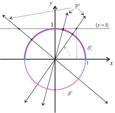
Figure 1: The geometry of the projective line and its parametrization. The double-headed arrows represent one-dimensional subspaces of the plane, i.e., elements of $\mathbb{P}^{1}$. The upper semi-circle $\mathcal{S}_{+}^{1}$ is shown in purple, its end-points in cyan, and the unit circle $\mathcal{S}^{1}$ in dashed magenta. The black points represent intersections of the lines with $y=1$ and with the unit circle, respectively.

Line fields arise in the computation of eigenvector fields for symmetric, second-order tensor fields [8, 32]. Eigenvectors have no intrinsic sign or length: only eigenspaces are well-defined at each point of the plane. Their orientation depends smoothly on their base point if the tensor field is smooth and has simple eigenvalues at that point. At repeated eigenvalues, isolated one-dimensional eigenspaces (and hence the corresponding values of the line field) become undefined.

Points to which a line field cannot be extended continuously are called singularities. These points are analogous to critical points of vector fields. Away from singularities, any smooth line field can locally be endowed with a smooth orientation. This implies the local existence of a normalized smooth vector field, which pointwise spans the respective line. Conversely, away from critical points, smooth vector fields induce smooth line fields when one takes their linear span pointwise.

Based on the index for planar vector fields, we introduce a notion of index for planar line fields following [30]. First, for some differentiable line field $\mathbf{l}$ and along some closed curve $\gamma\colon\mathcal{S}^{1}\to\mathds{R}^{2}$, pick at each point $\gamma(t)$ the representative upper half-plane vector from $\mathbf{l}(\gamma(t))$. This choice yields a normalized vector field along $\gamma$ which is as smooth as $\mathbf{l}$, except where $\mathbf{l}\circ\gamma$ crosses the horizontal subspace. At such a point, there is a jump-discontinuity in the representative vector from right to left or vice versa. To remove this discontinuity, the representative vectors are turned counter-clockwise by $\alpha\colon\mathcal{S}_{+}^{1}\to\mathcal{S}^{1}$, $\left(\cos 2\pi s\sin 2\pi s\right)\mapsto\left(\cos 4\pi s,\sin 4\pi s\right)$, $s\in[0,1/2]$, i.e., the parametrizing angle is doubled. Thereby, the left end-point with angle $\pi$ is mapped onto the right end-point with angle $0$. This representation $\alpha\circ\mathbf{l}$ permits the extension of the notion of index to planar line fields as follows.

Definition 2 (Index of a line field).

For a continuous, piecewise differentiable planar line field $\mathbf{l}\colon D\subseteq\mathds{R}^{2}\to\mathbb{P}^{1}$ and a simple closed curve $\gamma\colon\mathcal{S}^{1}\to\mathds{R}^{2}$, we define the index of  $\mathbf{l}$ along $\gamma$ as

$$\operatorname{ind}_{\gamma}(\mathbf{l})\coloneqq\frac{1}{2}\operatorname{ind}_{\gamma}(\alpha\circ\mathbf{l}).$$

The coefficient $1/2$ in this definition is needed to correct the doubling effect of $\alpha$. It also makes the index for a line field, generated by a vector field in the interior of $\gamma$, equal to the index of that vector field. Since Definition 2 refers to Definition 1, the additional definitions and properties described in Section 2 for vector fields carry over to line fields.

We call a curve $\gamma$ an orbit of $\mathbf{l}$, if it is everywhere tangent to $\mathbf{l}$. The scientific visualization community refers to orbits of lines fields arising from the eigenvectors of a symmetric tensor as tensor (field) lines or hyperorbit (trajectories) [8, 32, 34].

By definition, the index of singularities of line fields can be a half integer, as opposed to the vector field case, where only integer indices are possible. Also, two new types of singularities emerge in the line field case: wedges (type $W$) of index $+1/2$, and trisectors (type $T$) of index $-1/2$ [8, 32]. The geometry near these singularities is shown in Fig. 2.

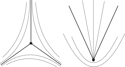
Figure 2: Orbit topologies in the vicinity of the two generic line field singularity types: trisector (left) and wedge (right). All lines represent orbits, the solid lines correspond to boundaries of hyperbolic sectors.

Node, centre, focus and saddle singularities also exist for line fields, but these singularities turn out to be structurally unstable with respect to small perturbations to the line field [8].

In this paper, we assume that only isolated singularities of the generic wedge and trisector types are present in the line field of interest. In that case, we obtain the following topological constraint on closed orbits of the line field.

Theorem 1.

Let $\mathbf{l}$ be a continuous, piecewise differentiable line field with only structurally stable singularities. Let $\Gamma$ be a closed orbit of  $\mathbf{l}$, and let $D$ denote the interior of $\Gamma$. We then have

$$W=T+2,$$ (1)

where $W$ and $T$ denote the number of wedges and trisectors, respectively, in $D$.

Proof.

First, $\Gamma$ has index $1$ with respect to $\mathbf{l}$, i.e., $\operatorname{ind}_{\Gamma}\left(\mathbf{l}\right)=1$. Second, its index equals the sum over all enclosed singularities, i.e.,

$$\sum_{i}\operatorname{ind}_{\Gamma}(p_{i},\mathbf{l})=\operatorname{ind}_{\Gamma}(\mathbf{l})=1.$$ (2)

Since we consider structurally stable singularities only, these are isolated and of either wedge or trisector type. From (2), we then obtain the equality

$$\frac{1}{2}\left(W-T\right)=1,$$

from which Eq. (1) follows. ∎

Consequently, in the interior of any closed orbit of a structurally stable line field, there are at least two singularities of wedge type, and exactly two more wedges than trisectors. Thus, a closed orbit necessarily encircles a wedge pair, and hence the existence of such a pair serves as a necessary condition in an automated search for closed orbits in line fields. In Fig. 3, we sketch two possible line field geometries in the interior of a closed orbit.

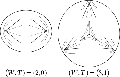
Figure 3: Possible topologies inside closed orbits: the $\left(W,T\right)=(2,0)$ configuration (left) and the $(3,1)$ configuration (right). In practice, we have only observed the simpler $(2,0)$ configuration.

4 Application to coherent Lagrangian vortex detection

Finding closed orbits in planar line fields is the decisive step in the detection of coherent Lagrangian vortices in a frame-invariant fashion [16, 3, 17]. Before describing the algorithmic scheme and showing results on ocean data, we briefly introduce the necessary background and notation for coherent Lagrangian vortices.

4.1 Flow map, Cauchy–Green strain tensor and $\lambda$–line field

We consider an unsteady, smooth, incompressible planar velocity field $\mathbf{u}(t,\mathbf{x})$ given on a finite time interval $\left[t_{0},t_{0}+T\right]$, and the corresponding equation of motion for the fluid,

$$\dot{\mathbf{x}}=\mathbf{u}(t,\mathbf{x}).$$

We denote the associated flow map by $\mathbf{F}_{t_{0}}^{t_{0}+T}$, which maps initial values $\mathbf{x}_{0}$ at time $t_{0}$ to their respective position at time $t_{0}+T$. Recall that the flow map is as smooth as the velocity field $\mathbf{u}$. Its linearisation can be used to define the Cauchy–Green strain tensor field

$$\mathbf{C}_{t_{0}}^{t_{0}+T}\coloneqq\left(D\mathbf{F}_{t_{0}}^{t_{0}+T}\right)^{\top}D\mathbf{F}_{t_{0}}^{t_{0}+T},$$

which is symmetric and positive-definite at each initial value. The eigenvalues and eigenvectors of $\mathbf{C}_{t_{0}}^{t_{0}+T}$ characterize the magnitude and directions of maximal and minimal stretching locally in the flow. We refer to these positive eigenvalues as $\lambda_{1}\leq\lambda_{2}$, with the associated eigenspaces spanned by the normalized eigenvectors $\xi_{1}$ and $\xi_{2}$.

As argued by [17], the positions of coherent Lagrangian vortex boundaries at time $t_{0}$ are closed stationary curves of the averaged tangential strain functional computed from $\mathbf{C}_{t_{0}}^{t_{0}+T}$. All stationary curves of this functional turn out to be uniformly stretched by a factor of $\lambda>0$ under the flow map $\mathbf{F}_{t_{0}}^{t_{0}+T}$. These stationary curves can be computed as closed orbits of the $\lambda$–line fields $\eta_{\lambda}^{\pm}$, spanned by the representing vector fields

$$\eta_{\lambda}^{\pm}\coloneqq\sqrt{\frac{\lambda_{2}-\lambda^{2}}{\lambda_{2}-\lambda_{1}}}\xi_{1}\pm\sqrt{\frac{\lambda^{2}-\lambda_{1}}{\lambda_{2}-\lambda_{1}}}\xi_{2}.$$ (3)

We refer to orbits of $\eta_{\lambda}^{\pm}$ as $\lambda$–lines. In the special case of $\lambda=1$, the line field $\eta_{1}^{\pm}$ coincides with the shear line field defined in [16], provided that the fluid velocity field $\mathbf{u}(t,\mathbf{x})$ is incompressible.

We refer to points at which the Cauchy–Green strain tensor is isotropic (i.e., equals a constant multiple of the identity tensor) as Cauchy–Green singularities. For incompressible flows, only $\mathbf{C}_{t_{0}}^{t_{0}+T}=\mathbf{I}$ is possible at Cauchy–Green singularities, implying $\lambda_{1}=\lambda_{2}=1$ at these points. The associated eigenspace fields, $\xi_{1}$ and $\xi_{2}$, are ill-defined as line fields at Cauchy–Green singularities, thus generically the line fields $\xi_{1}$, $\xi_{2}$ and $\eta_{1}^{\pm}$ have singularities at these points. Conversely, the singularities of the line fields $\xi_{1}$, $\xi_{2}$ and $\eta_{1}^{\pm}$ are necessarily Cauchy–Green singularities, as seen from the local vector field representation in Eq. (3).

Following [16, 17], we define an elliptic Lagrangian Coherent Structure (LCS) as a structurally stable closed orbit of $\eta_{\lambda}^{\pm}$ for some choice of the $\pm$ sign, and for some value of the parameter $\lambda$. We then define a (coherent Lagrangian) vortex boundary as the locally outermost elliptic LCS over all choices of $\lambda$.

4.2 Index theory for $\lambda$–line fields

In regions where $\lambda_{1}<\lambda^{2}<\lambda_{2}$ is not satisfied, $\eta_{\lambda}^{\pm}$ is undefined. Such open regions necessarily arise around Cauchy–Green singularities, and hence $\eta_{\lambda}^{\pm}$ does not admit isolated point-singularities. Consequently, the index theory presented in Section 3 does not immediately apply to the $\lambda$–line field. We show below, however, that Cauchy–Green singularities are still necessary indicators of closed orbits of $\eta_{\lambda}^{\pm}$ for arbitrary $\lambda$.

For $\lambda>1$, the set $D_{\lambda}^{2}=\left\{\lambda_{2}<\lambda^{2}\right\}$, on which $\eta_{\lambda}^{\pm}$ is undefined, consists of open connected components. All Cauchy–Green singularities are contained in some of these $D_{\lambda}^{2}$-components. A priori, however, there may exist $D_{\lambda}^{2}$-components that do not contain Cauchy–Green singularities.

On the boundary $\partial D_{\lambda}^{2}$, we have $\lambda_{2}=\lambda^{2}$, and hence $\eta_{\lambda}^{\pm}$ coincides with $\xi_{2}$ on $\partial D_{\lambda}^{2}$, as shown in Fig. 4. Therefore, we may extend $\eta_{\lambda}^{\pm}$ into $D_{\lambda}^{2}$ by letting $\eta_{\lambda}^{\pm}(\mathbf{x})\coloneqq\xi_{2}(\mathbf{x})$ for all $\mathbf{x}\in D_{\lambda}^{2}$, thereby obtaining a continuous, piecewise differentiable line field, whose singularity positions coincide with those of the $\xi_{2}$-singularities.

Theorem 1 applies directly to the continuation of the line field $\eta_{\lambda}^{\pm}$, and enables the detection of closed orbits lying outside the open set $D_{\lambda}^{2}$. In the case $\lambda<1$, the line field $\eta_{\lambda}^{\pm}$ can similarly be extended in a continuous fashion into the interior of the set $D_{\lambda}^{1}=\left\{\lambda_{1}>\lambda^{2}\right\},$ through the definition $\eta_{\lambda}^{\pm}(\mathbf{x})\coloneqq\xi_{1}(\mathbf{x})$ for all $\mathbf{x}\in D_{\lambda}^{1}$.

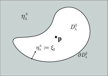
Figure 4: The original domain of definition of $\eta_{\lambda}^{\pm}$ (grey), and the domain $D_{\lambda}^{2}$ (white), to which $\eta_{\lambda}^{\pm}$ can be continuously extended via the line field $\xi_{2}$. Also shown is a point $\mathbf{p}$ denoting a Cauchy–Green singularity.

After its extension into the set $D_{\lambda}=D_{\lambda}^{1}\cup D_{\lambda}^{2}$, the line field $\eta_{\lambda}^{\pm}$ inherits each Cauchy–Green singularity either from $\xi_{2}$ or from $\xi_{1}$. A priori, the same Cauchy–Green singularity may have different topological types in the $\xi_{1}$ and $\xi_{2}$ line fields. By [7, Theorem 11], however, this is not the case: corresponding generic singularities of $\xi_{2}$ and $\xi_{1}$ share the same index and have the same number of hyperbolic sectors. Furthermore, the separatrices of the $\xi_{2}$-singularity are obtained from the separatrices of the $\xi_{1}$-singularity by reflection with respect to the singularity. In summary, $\xi_{1}$-wedges correspond exactly to $\xi_{2}$-wedges, and the same holds for trisectors. For the singularity type classification for $\eta_{\lambda}^{\pm}$, $\lambda\neq 1$, we may therefore pick $\xi_{2}$, irrespective of the sign of $\lambda-1$.

The singularity-type correspondence extends also to the limit case $\lambda=1$, i.e., to $\eta_{1}^{\pm}$, as follows. Consider the one-parameter family of line-field extensions $\eta_{\lambda}^{\pm}$. By construction, the locations of $\eta_{\lambda}^{\pm}$ point singularities coincide with those of the $\xi_{2}$-singularities for any $\lambda$. Variations of $\lambda$ correspond to continuous line-field perturbations, which leave the types of structurally stable singularities unchanged. Hence, the types of $\eta_{1}^{\pm}$-singularities must match the types of corresponding $\eta_{\lambda}^{\pm}$-singularities, or equivalently of corresponding $\xi_{2}$-singularities. To summarize, we obtain the following conclusion.

Proposition 1.

Any closed orbit of a structurally stable $\eta_{\lambda}^{\pm}$ field necessarily encircles Cauchy–Green singularities satisfying Eq. (1).

4.3 A simple example: coherent Lagrangian vortex in the double gyre flow

We consider the left vortex of the double gyre flow [29], defined on the spatial domain $[0,1]\times[0,1]$ by the ODE

$$\dot{x} =-\pi A\sin(\pi f(x))\cos(\pi y),$$

$$\dot{y} =\pi A\cos(\pi f(x))\sin(\pi y)\partial_{x}f(t,x),$$

where

$$f(t,x)=\varepsilon\sin(\omega t)x^{2}+\left(1-2\varepsilon\sin(\omega t)\right)x.$$

We choose the parameters of the flow model as $A=0.2$, $\varepsilon=0.2$, $\omega=\pi/5$, $t_{0}=0$, and $T=5\pi/2$.

In the $\lambda$–line field shown in Fig. 5(a), we identify a pair of wedge singularities. Any closed $\lambda$–line must necessarily enclose this pair by Proposition 1. This prompts us to define a Poincaré section through the midpoint of the connecting line between the two wedges. For computational simplicity, we select the Poincaré section as horizontal. Performing a parameter sweep over $\lambda$–values, we obtain the outermost closed orbit shown in Fig. 5(a) for a uniform stretching rate of $\lambda=0.975$. Other non-closing orbits and the $\lambda$–line field are also shown for illustration. In addition, we show the line field topology around the wedge pair in the vortex core in Fig. 5(b).

In this simple example, the vortex location is known, and hence a Poincaré section could manually be set for closed orbit detection in the $\lambda$–line fields. In more complex flows, however, the vortex locations are a priori unknown, making a manual search unfeasible.

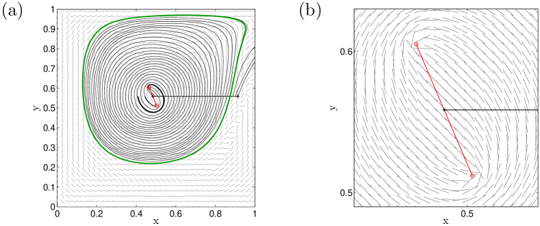
Figure 5: (a) Vortex boundary ($\lambda=0.975$) for the left vortex of the double gyre flow. In the centre, the pair of wedge singularities (red) determines the topology of the $\lambda$–line field $\eta_{\lambda}^{-}$ (grey) and therefore indicates a candidate region for closed orbits. The $\lambda$–lines (black) are launched from the Poincaré section (black crosses) to find the outermost closed orbit (green). (b) A blow-up of the centre of the vortex with the detailed circular topology of the $\lambda$–line field $\eta_{\lambda}^{-}$ in the vicinity of the $(2,0)$ wedge pair configuration (cf. Fig. 3).

4.4 Implementation for vortex census in large-scale ocean data

Our automated Lagrangian vortex-detection scheme relies on Proposition 1, identifying candidate regions in which Poincaré maps for closed $\lambda$–line detection should be set up. In several tests on ocean data, we only found the $(W,T)=(2,0)$ singularity configuration inside closed $\lambda$–lines. This is consistent with our previous genericity considerations. Consequently, we focus on finding candidate regions for closed $\lambda$–lines as regions with isolated pairs of wedges in the $\xi_{2}$ field. In the following, we describe the procedure for an automated detection of closed $\lambda$–lines.

1. Locate singularities.

Recall that Cauchy–Green singularities are points where$\mathbf{C}_{t_{0}}^{t_{0}+T}=\mathbf{I}$. We find such points at subgrid-resolution as intersections of the zero level sets of the functions $c_{1}\coloneqq C_{11}-C_{22}$ and $c_{2}\coloneqq C_{12}=C_{21}$, where $C_{ij}$ denote the entries of the Cauchy–Green strain tensor.

2. Select relevant singularities.

We focus on generic singularities, which are isolated and are of wedge or trisector type. We discard tightly clustered groups of singularities, which indicate non-elliptic behavior in that region. Effectively, the clustering of singularities prevents the reliable determination of their singularity type. To this end, we select a minimum distance threshold between admissible singularities as $2\Delta x$, where $\Delta x$ denotes the grid size used in the computation of $\mathbf{C}_{t_{0}}^{t_{0}+T}$. We obtain the distances between closest neighbours from a Delaunay triangulation procedure.

3. Determine singularity type.

Singularities are classified as trisectors or wedges, following the approach developed in [10]. Specifically, a circular neighbourhood of radius $r>0$ is selected around a singularity, so that no other singularity is contained in this neighbourhood. With a rotating radius vector $\mathbf{r}$ of length $r$, we compute the absolute value of the cosine of the angle enclosed by $\mathbf{r}$ and $\xi_{2}$, i.e., $\cos\left(\angle\left(\mathbf{r},\xi_{2}\right)\right)=\left|\mathbf{r}\cdot\xi_{2}\right|/r$, with the eigenvector field $\xi_{2}$ interpolated linearly to 1000 positions on the radius $r$ circle around the singularity. The singularity is classified as a trisector, if $\mathbf{r}$ is orthogonal to $\xi_{2}$ at exactly three points of the circle, and parallel to $\xi_{2}$ at three other points, which mark separatrices of the trisector (Fig. 2). Singularities not passing this test for trisectors are classified as wedges. Other approaches to singularity classification can be found in [8] and [2], which we have found too sensitive for oceanic data sets.

4. Filter

We discard wedge points whose closest neighbour is of trisector-type, because these wedge points cannot be part of an isolated wedge pair. We further discard single wedges whose distance to the closest wedge point is larger than the typical mesoscale distance of $2\,^{\circ}\approx 200$ km. The remaining wedge pairs mark candidate regions for elliptic LCS (Fig. 6(a)).

5. Launch $\lambda$–lines from a Poincaré-section

We set up Poincaré sections that span from the midpoint of a wedge pair to a point $1.5\,^{\circ}$ apart in longitudinal direction (Fig. 6(b)). This choice of length for the Poincaré section captures eddies up to a diameter of $3\,^{\circ}\approx 300$ km, an upper bound on the accepted size for mesoscale eddies. For a fixed $\lambda$–value, $\lambda$–lines are launched from 100 initial positions on the Poincaré section, and the return distance $P(x)-x$ is computed. Zero crossings of the return distance function correspond to closed $\lambda$–lines. The position of zeros is subsequently refined on the Poincaré section through the bisection method. The outermost zero crossing of the return distance marks the largest closed $\lambda$–line for the chosen $\lambda$–value. To find the outermost closed $\lambda$–line over all $\lambda$–values, we vary $\lambda$ from $0.85$ to $1.15$ in $0.01$ steps, and pick the outermost closed orbit as the Lagrangian eddy boundary. During this process, we make sure that eddy boundaries so obtained do enclose the two wedge singularities used in the construction, but no other singularities.

The runtime of our algorithm is dominated by the fifth step, the integration of $\lambda$–lines, as illustrated in Table 1 for the ocean data example in the next section. This is the reason why our investment in the selection, classification and filtering of singularities before the actual $\lambda$–line integration pays off.

4.5 Coherent Lagrangian vortices in an ocean surface flow

We now apply the method summarized in steps 1-5 above to two-dimensional unsteady velocity data obtained from AVISO satellite altimetry measurements. The domain of the data set is the Agulhas leakage in the Southern Ocean, represented by large coherent eddies that pinch off from the Agulhas current of the Indian Ocean.

Under the assumption of a geostrophic flow, the sea surface height $h$ serves as a streamfunction for the surface velocity field. In longitude-latitude coordinates $(\varphi,\theta)$, particle trajectories are then solutions of

$$\dot{\varphi} =-\frac{\mathrm{g}}{\mathrm{R}^{2}f(\theta)\cos\theta}\partial_{\theta}h(\varphi,\theta,t), \dot{\theta} =\frac{\mathrm{g}}{\mathrm{R}^{2}f(\theta)\cos\theta}\partial_{\varphi}h(\varphi,\theta,t),$$

where $\mathrm{g}$ is the constant of gravity, $\mathrm{R}$ is the mean radius of the Earth, and $f(\theta)\coloneqq 2\Omega\sin\theta$ is the Coriolis parameter, with $\Omega$ denoting the Earth’s mean angular velocity. For comparison, we choose the same spatial domain and time interval as in [3, 17]. The integration time $T$ is also set to $90$ days.

Fig. 6 illustrates the steps of the eddy detection algorithm. From all singularities of the Cauchy–Green strain tensor, isolated wedge pairs are extracted (Fig. 6(a)) and closed orbits are found by launching $\lambda$–lines from Poincaré sections anchored at those wedge pairs (Fig. 6(b)). Altogether, 14 out of the selected wedge pairs are encircled by closed orbits and, hence, by coherent Lagrangian eddy boundaries (Fig. 6(c)). The reduction to candidate regions consistent with Proposition 1 leads to significant gain in computational speed. This is because the computationally expensive integration of the $\lambda$–line field is only carried out in these regions (Table 1). For comparison, the computational cost on a single Poincaré section is already higher than the cost of identifying the candidate regions. Note also that two regions contain three wedges, which constitute two admissible wedge pairs. This explains how 78 wedges constitute 40 wedge pairs altogether.

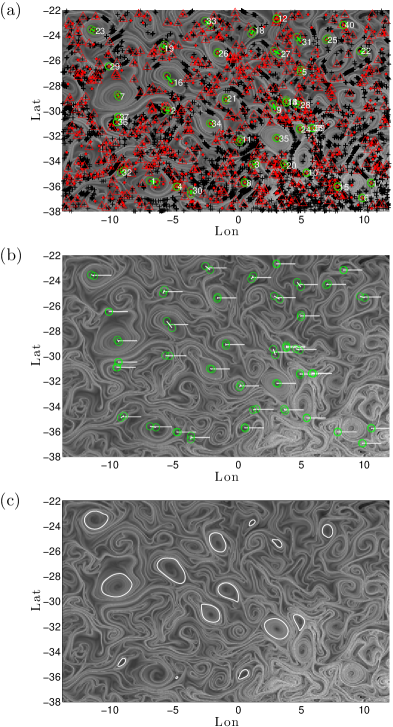
Figure 6: Visualization of the eddy detection algorithm for an ocean surface flow. (a) Singularities of the Cauchy–Green strain tensor of trisector type (red triangles) and wedge type (green circles: kept, red dots: discarded). Wedge pairs are candidate cores of coherent eddies. A total of 40 wedge pairs were finally selected for further analysis out of all singularities (black crosses) by the procedure described in Section 4.4. (b) Poincaré sections anchored at the centre of the selected wedge pairs. Coherent vortex boundaries are found as closed $\lambda$–lines intersecting these Poincaré sections. (c) Boundaries of 14 coherent eddies on November 24, 2006. The $\log_{10}\lambda_{2}$ field is shown in the background as an illustration of the stretching distribution in the flow.

	Runtime	Number of points
1. Localization	$11.0$ s	14,211 singularities
2. Selection	$12.8$ s	912 singularities
3. Classification	$85.9$ s	414 wedges
4. Filtering	$0.5$ s	78 wedges
5. Integration	$\sim 200$ s / wedge pair / $\lambda$–value	40 wedge pairs
End result	—	14 eddies

Table 1: Runtime of the algorithm for the Agulhas data set on a CPU with 2.2 GHz and 32 GB RAM. Since the integration of $\lambda$–lines is the computationally most expensive part, the reduction of the number of candidate regions to only 40 by application of index theory yields a significant computational advantage.

5 Conclusion

We have discussed the use of index theory in the detection of closed orbits in planar line fields. Combined with physically motivated filtering criteria, index-based elliptic LCS detection provides an automated implementation of the variational results of [17] on coherent Lagrangian vortex boundaries. Our results further enhance the power of LCS detection algorithms already available in the Matlab toolbox LCS TOOL (cf. [21]).

Our approach can be extended to three-dimensional flows, where line fields arise in the computation of intersections of elliptic LCS with two-dimensional planes [4]. Applied over several such planes, our approach allows for an automated detection of coherent Lagrangian eddies in three-dimensional unsteady velocity fields.

Automated detection of Lagrangian coherent vortices should lead to precise estimates on the volume of water coherently carried by mesoscale eddies, thereby revealing the contribution of coherent eddy transport to the total flux of volume, heat and salinity in the ocean. Related work is in progress.

References

- [1] M. R. Allshouse and J.-L. Thiffeault. Detecting coherent structures using braids. Physica D, 241(2):95–105, 2012.
- [2] A.M. Bazen and S.H. Gerez. Systematic methods for the computation of the directional fields and singular points of fingerprints. IEEE Trans. Pattern Anal. Machine Intell., 24(7):905–919, 2002.
- [3] F. J. Beron-Vera, Y. Wang, M. J. Olascoaga, G. J. Goni, and G. Haller. Objective detection of oceanic eddies and the Agulhas leakage. J. Phys. Oceanogr., 43(7):1426–1438, 2013.
- [4] D. Blazevski and G. Haller. Hyperbolic and elliptic transport barriers in three-dimensional unsteady flows. Physica D, 273-274(0):46–62, 2014.
- [5] D. B. Chelton, M. G. Schlax, R. M. Samelson, and R. A. de Szoeke. Global observations of large oceanic eddies. Geophysical Research Letters, 34(15):L15606, 2007.
- [6] W. P. M. de Ruijter, A. Biastoch, S. S. Drijfhout, J. R. E. Lutjeharms, R. P. Matano, T. Pichevin, P. J. van Leeuwen, and W. Weijer. Indian-Atlantic interocean exchange: Dynamics, estimation and impact. Journal of Geophysical Research: Oceans, 104(C9):20885–20910, 1999.
- [7] T. Delmarcelle. The Visualization of Second-Order Tensor Fields. PhD thesis, Stanford University, 1994.
- [8] T. Delmarcelle and L. Hesselink. The topology of symmetric, second-order tensor fields. In Proceedings of the conference on Visualization ’94, VIS ’94, pages 140–147. IEEE Computer Society Press, 1994.
- [9] C. Dong, J. C. McWilliams, Y. Liu, and D. Chen. Global heat and salt transports by eddy movement. Nature Communications, 5(3294):1–6, 2014.
- [10] M. Farazmand, D. Blazevski, and G. Haller. Shearless transport barriers in unsteady two-dimensional flows and maps. Physica D, 278-279:44–57, 2014.
- [11] M. Farazmand and G. Haller. How coherent are the vortices of two-dimensional turbulence? 2014. submitted preprint.
- [12] G. Froyland. An analytic framework for identifying finite-time coherent sets in time-dependent dynamical systems. Physica D, 250(0):1 – 19, 2013.
- [13] G. Froyland, C. Horenkamp, V. Rossi, N. Santitissadeekorn, and A. Sen Gupta. Three-dimensional characterization and tracking of an Agulhas Ring. Ocean Modelling, 52-53:69–75, 2012.
- [14] G. Froyland, N. Santitissadeekorn, and A. Monahan. Transport in time-dependent dynamical systems: Finite-time coherent sets. Chaos, 20(4):043116, 2010.
- [15] G. Haller. An objective definition of a vortex. Journal of Fluid Mechanics, 525:1–26, 1 2005.
- [16] G. Haller and F. J. Beron-Vera. Geodesic theory of transport barriers in two-dimensional flows. Physica D, 241(20):1680–1702, 2012.
- [17] G. Haller and F. J. Beron-Vera. Coherent Lagrangian vortices: the black holes of turbulence. J. Fluid Mech., 731:R4, 2013.
- [18] J. M. Lee. Introduction to Smooth Manifolds, volume 218 of Graduate Texts in Mathematics. Springer, 2nd edition, 2012.
- [19] C. Mendoza and A. M. Mancho. Hidden Geometry of Ocean Flows. Physical Review Letters, 105(3):038501–, 2010.
- [20] T. Needham. Visual complex analysis. Oxford University Press, 2000.
- [21] K. Onu, F. Huhn, and G. Haller. An Algorithmic Introduction to Lagrangian Coherent Structures. 2014. submitted.
- [22] T. Peacock and J. Dabiri. Introduction to Focus Issue: Lagrangian Coherent Structures. Chaos, 20(1):017501, 2010.
- [23] T. Peacock and G. Haller. Lagrangian coherent structures: The hidden skeleton of fluid flows. Physics Today, 66(2):41–47, 2013.
- [24] L. Perko. Differential Equations and Dynamical Systems, volume 7 of Texts in Applied Mathematics. Springer, 3rd edition, 2001.
- [25] M. R. Petersen, S. J. Williams, M. E. Maltrud, M. W. Hecht, and B. Hamann. A three-dimensional eddy census of a high-resolution global ocean simulation. Journal of Geophysical Research: Oceans, 118(4):1759–1774, 2013.
- [26] S.V. Prants, V.I. Ponomarev, M.V. Budyansky, M.Yu. Uleysky, and P.A. Fayman. Lagrangian analysis of mixing and transport of water masses in the marine bays. Izvestiya, Atmospheric and Oceanic Physics, 49(1):82–96, 2013.
- [27] A. Provenzale. Transport by Coherent Barotropic Vortices. Annual Review of Fluid Mechanics, 31(1):55–93, 1999.
- [28] I. I. Rypina, S. E. Scott, L. J. Pratt, and M. G. Brown. Investigating the connection between complexity of isolated trajectories and Lagrangian coherent structures. Nonlinear Processes in Geophysics, 18(6):977–987, 2011.
- [29] S. C. Shadden, F. Lekien, and J. E. Marsden. Definition and properties of Lagrangian coherent structures from finite-time Lyapunov exponents in two-dimensional aperiodic flows. Physica D, 212(3-4):271–304, 2005.
- [30] M. Spivak. A Comprehensive Introduction to Differential Geometry, volume 3. Publish or Perish, Inc., 3rd edition, 1999.
- [31] P. Tallapragada and S. D. Ross. A set oriented definition of finite-time Lyapunov exponents and coherent sets. Communications in Nonlinear Science and Numerical Simulation, 18(5):1106–1126, 2013.
- [32] X. Tricoche, X. Zheng, and A. Pang. Visualizing the Topology of Symmetric, Second-Order, Time-Varying Two-Dimensional Tensor Fields. In J. Weickert and H. Hagen, editors, Visualization and Processing of Tensor Fields, Mathematics and Visualization, pages 225–240. Springer, 2006.
- [33] J. Weickert and H. Hagen, editors. Visualization and Processing of Tensor Fields. Mathematics and Visualization. Springer, 2006.
- [34] T. Wischgoll and J. Meyer. Locating Closed Hyperstreamlines in Second Order Tensor Fields. In J. Weickert and H. Hagen, editors, Visualization and Processing of Tensor Fields, Mathematics and Visualization, pages 257–267. Springer, 2006.
- [35] T. Wischgoll and G. Scheuermann. Detection and visualization of closed streamlines in planar flows. IEEE Trans. Visual. Comput. Graphics, 7(2):165–172, 2001.
- [36] C. L. Wolfe and P. Cessi. Overturning Circulation in an Eddy-Resolving Model: The Effect of the Pole-to-Pole Temperature Gradient. Journal of Physical Oceanography, 39(1):125–142, 2009.
- [37] L. Zhang, Q. Deng, R. Machiraju, A. Rangarajan, D. Thompson, D. K. Walters, and H.-W. Shen. Boosting Techniques for Physics-Based Vortex Detection. Computer Graphics Forum, 33(1):282–293, 2014.
- [38] Z. Zhang, W. Wang, and B. Qiu. Oceanic mass transport by mesoscale eddies. Science, 345(6194):322–324, 2014.