Thermal balance and photon-number quantization in layered structures

Abstract

The quantization of the electromagnetic field in lossy and dispersive dielectric media has been widely studied during the last few decades. However, several aspects of energy transfer and its relation to consistently defining position-dependent ladder operators for the electromagnetic field in nonequilibrium conditions have partly escaped the attention. In this work we define the position-dependent ladder operators and an effective local photon-number operator that are consistent with the canonical commutation relations and use these concepts to describe the energy transfer and thermal balance in layered geometries. This approach results in a position-dependent photon-number concept that is simple and consistent with classical energy conservation arguments. The operators are formed by first calculating the vector potential operator using Green’s function formalism and Langevin noise source operators related to the medium and its temperature, and then defining the corresponding position-dependent annihilation operator that is required to satisfy the canonical commutation relations in arbitrary geometry. Our results suggest that the effective photon number associated with the electric field is generally position dependent and enables a straightforward method to calculate the energy transfer rate between the field and the local medium. In particular, our results predict that the effective photon number in a vacuum cavity formed between two lossy material layers can oscillate as a function of the position suggesting that also the local field temperature oscillates. These oscillations are expected to be directly observable using relatively straightforward experimental setups in which the field-matter interaction is dominated by the coupling to the electric field. The approach also gives further insight on separating the photon ladder operators into the conventional right and left propagating parts and on the anomalies reported for the commutation relations of the corresponding operators within optical cavities.

I Introduction

Recent research of nanoscale radiative energy transfer has enabled advances and in-depth insight in several fields of optical technologies related, e.g., to nanoplasmonics Sorger and Zhang (2011); Oulton et al. (2009); Huang et al. (2013); Sadi et al. (2013), near-field microscopy Taubner et al. (2006); Hillenbrand et al. (2002), thin-film light-emitting diodes Nakamura and Krames (2013); Heikkilä et al. (2013), photonic crystals Russell (2003); Akahane et al. (2003), and metamaterials Tanaka et al. (2010); Mattiucci et al. (2013). The optical phenomena taking place in nanoscale also naturally lead to questions related to the quantum nature of light, proper ways to quantize the fields, and maybe even more importantly on how to interpret the results. The research related to quantum optics of nanoscale systems is strongly influenced by the availability of simple and transparent theoretical tools and models that allow in-depth understanding of the pertinent phenomena in sufficiently simple form. Such insight has been used, for instance, in the recent demonstrations and studies of noiseless but nondeterministic optical amplifiers Zavatta et al. (2011); Ferreyrol et al. (2010); Partanen et al. (2012) and optical properties of cavities Gröblacher et al. (2009); Collette et al. (2013); Häyrynen et al. (2011, 2009). Simple description of the quantum aspects of energy transfer is especially interesting and challenging in lossy nanoscale systems often simulated by the prototypical one-dimensional lossy structures.

The research of quantum optical processes in such lossy systems during the last few decades has generated a wealth of information on the quantization of the electromagnetic (EM) field in dielectrics and especially in layered structures. In the context of the present work, the most relevant quantization approach has focused on the input–output relation formalism (IORF) of the photon creation and annihilation operators providing a detailed description of the spatial field evolution. The formalism was originally developed for dispersionless and lossless dielectrics by Knöll et al. Knöll et al. (1987) and soon extended for lossy and dispersive media for the study of passive optical devices, such as dielectric plates, interfaces, and optical cavities by several groups Knöll et al. (1991); Allen and Stenholm (1992); Huttner and Barnett (1992); Barnett and Loudon (1995); Matloob et al. (1995); Matloob and Loudon (1996). The complete quantization procedures studied, e.g., by Barnett et al. Barnett and Loudon (1995) fully accounting for the coupling between the EM field and the states of homogeneous lossy media clearly highlighted that the noise and field operators in lossy systems became position dependent. The vector potential and electric field operators in the above works obeyed the well-known canonical commutation relation for an arbitrary choice of normal mode functions as expected Barnett and Loudon (1995); Matloob et al. (1995), but the commutation relations of the ladder operators did not. The anomalous commutation relations of the ladder operators were studied in several reports Raymer and McKinstrie (2013); Barnett et al. (1996); Ueda and Imoto (1994); Aiello (2000); Di Stefano et al. (2000) but no clear resolution for the anomalies was found apart from reaching a consensus that the anomalies were irrelevant as long as the field commutation relations and classical field quantities were well defined. Since then, the IORF has mainly been applied in calculating the classical field quantities until the very recent suggestions that, despite the early interpretations, the ladder operators and their commutation relations might in fact relate to measurable physical properties Collette et al. (2013).

In this paper, we define position-dependent ladder operators associated with the vector potential in a way that is consistent with the canonical commutation relations. The introduced position-dependent annihilation and photon-number operators give further insight on the local effective photon number, thermal balance, and the formation of the local thermal equilibrium. We focus on thermal source fields, but in principle the introduced operators also allow one to investigate fields with other kinds of quantum statistics. We also discuss the possibility of dividing the photon number into left and right propagating parts, and the origin of the anomalies reported in cavity operators based on this division. The approach that is initially based on purely mathematical arguments is also shown to result in a physically meaningful definition of the photon number that has a very attractive and simple connection to the field temperature and thermal balance of the system.

The paper is organized as follows. In Sec. II the theoretical background is briefly reviewed and the position-dependent ladder and photon-number operators satisfying the canonical commutation relations are defined. To enable comparison between the conventional field operators and the position-dependent photon-number operator we also briefly review the concepts for the energy density and Poynting vector in lossy, dispersive media. In addition, we show how the introduced effective photon-number operator is related to the thermal balance of the system. In Sec. III, the presented theoretical concepts are applied to study the position dependence of the photon number, electric field fluctuation, electrical contribution of the local density of EM states, energy density, Poynting vector, and net emission rate in the geometries of an interface separating a lossy medium from vacuum and a vacuum cavity between lossy media.

II Field quantization

II.1 Overview of the noise operator formalism for EM field quantization

Field quantization in lossy dielectrics is well established, but for the purposes of the present discussion it is convenient to briefly review some of the key results and theoretical background for the quantization of the EM field in one dimension. In this section, we give an overview of the results originally presented by Matloob et al. Matloob et al. (1995) to lay the ground for defining the position-dependent ladder and photon-number operators and the related discussion in the following sections.

The electromagnetic waves are considered to propagate parallel to the $x$ axis with their transverse electric and magnetic vector operators $\hat{E}(x,t)$ and $\hat{B}(x,t)$ parallel to the $y$ and $z$ axes, respectively. The field operators are related to the vector potential operator $\hat{A}(x,t)$ by the relations Matloob et al. (1995)

$$\hat{E}^{+}(x,\omega) =i\omega\hat{A}^{+}(x,\omega),$$ (1)

$$\hat{B}^{+}(x,\omega) =\frac{\partial}{\partial x}\hat{A}^{+}(x,\omega)$$ (2)

for positive frequencies. The negative frequency parts $\hat{E}^{-}(x,\omega)$, $\hat{B}^{-}(x,\omega)$, and $\hat{A}^{-}(x,\omega)$ are Hermitian conjugates of the positive frequency parts.

The field operators satisfy the frequency domain Maxwell’s equations and, when the relations in Eqs. (1) and (2) are used, the vector potential operator can be shown to satisfy the one-dimensional nonhomogeneous Helmholtz equation Matloob et al. (1995)

$$\frac{\partial^{2}}{\partial x^{2}}\hat{A}^{+}(x,\omega)+\frac{\omega^{2}n(x,\omega)^{2}}{c^{2}}\hat{A}^{+}(x,\omega)=-\mu_{0}\hat{J}_{\mathrm{em}}(x,\omega),$$ (3)

where $\mu_{0}$ is the permeability of vacuum, $n(x,\omega)$ is the refractive index of the medium, and $\hat{J}_{\mathrm{em}}(x,\omega)=j_{0}(x,\omega)\hat{f}(x,\omega)$ is a Langevin noise current operator presented in terms of the scaling factor $j_{0}(x,\omega)$ and the modified Langevin force operator $\hat{f}(x,\omega)$, which is a bosonic field operator defined through the following commutation relations:

$$[\hat{f}(x,\omega),\hat{f}^{\dagger}(x^{\prime},\omega^{\prime})] =\delta(x-x^{\prime})\delta(\omega-\omega^{\prime}),$$ (4)

$$[\hat{f}(x,\omega),\hat{f}(x^{\prime},\omega^{\prime})] =[\hat{f}^{\dagger}(x,\omega),\hat{f}^{\dagger}(x^{\prime},\omega^{\prime})]=0.$$ (5)

The scaling factor of the Langevin noise current operator is given by $j_{0}(x,\omega)=\sqrt{4\pi\hbar\omega^{2}\varepsilon_{0}\mathrm{Im}[n(x,\omega)^{2}]/S}$, where $\hbar$ is the reduced Planck’s constant, $\varepsilon_{0}$ is the permittivity of vacuum, and $S$ is the area of quantization in the $y$-$z$ plane Matloob et al. (1995). The magnitude of the scaling factor has been determined by requiring that the vector potential and electric field operators obey the canonical equal-time commutation relation as detailed in Ref. Matloob et al. (1995).

The solution to Eq. (3) can be written in terms of the Green’s function of the Helmholtz equation as

$$\hat{A}^{+}(x,\omega)=\mu_{0}\int_{-\infty}^{\infty}j_{0}(x^{\prime},\omega)G(x,\omega,x^{\prime})\hat{f}(x^{\prime},\omega)dx^{\prime}.$$ (6)

The Green’s function depends on the problem geometry via the refractive index of the medium. For example, in a homogeneous space the Green’s function can be written as

$$G(x,\omega,x^{\prime})=\frac{ie^{ik(\omega)|x-x^{\prime}|}}{2k(\omega)},$$ (7)

where $k(\omega)=\omega n(\omega)/c$ is the wave vector. The Green’s functions for the selected layered structures are given in the Appendix.

In order to write the field operators in compact forms, we define the scaled forms of the Green’s functions:

$$G_{\mathrm{A}}(x,\omega,x^{\prime})=\; \mu_{0}j_{0}(x^{\prime},\omega)G(x,\omega,x^{\prime}),$$ (8)

$$G_{\mathrm{E}}(x,\omega,x^{\prime})=\; i\mu_{0}\omega j_{0}(x^{\prime},\omega)G(x,\omega,x^{\prime}),$$ (9)

$$G_{\mathrm{B}}(x,\omega,x^{\prime})=\; \frac{i\mu_{0}\omega n(x,\omega)}{c}j_{0}(x^{\prime},\omega)$$

$$\times[G_{\mathrm{R}}(x,\omega,x^{\prime})-G_{\mathrm{L}}(x,\omega,x^{\prime})],$$ (10)

where $G_{\mathrm{E}}(x,\omega,x^{\prime})$ and $G_{\mathrm{B}}(x,\omega,x^{\prime})$ are obtained from $G_{\mathrm{A}}(x,\omega,x^{\prime})$ by using Eqs. (1) and (2), and $G_{\mathrm{R}}(x,\omega,x^{\prime})$ and $G_{\mathrm{L}}(x,\omega,x^{\prime})$ are the right and left propagating parts of the Green’s function identified from the factors $e^{ikx}$ and $e^{-ikx}$, respectively. In this paper, when treating lossless semi-infinite media, an infinitesimal imaginary part of the refractive index is assumed in $j_{0}(x,\omega)$ and $G(x,\omega,x^{\prime})$ and it is set to zero after calculating the integrals. Using the above definitions the field operators are given by

$$\hat{A}^{+}(x,\omega) =\int_{-\infty}^{\infty}G_{\mathrm{A}}(x,\omega,x^{\prime})\hat{f}(x^{\prime},\omega)dx^{\prime},$$ (11)

$$\hat{E}^{+}(x,\omega) =\int_{-\infty}^{\infty}G_{\mathrm{E}}(x,\omega,x^{\prime})\hat{f}(x^{\prime},\omega)dx^{\prime},$$ (12)

$$\hat{B}^{+}(x,\omega) =\int_{-\infty}^{\infty}G_{\mathrm{B}}(x,\omega,x^{\prime})\hat{f}(x^{\prime},\omega)dx^{\prime}.$$ (13)

In time domain the fields are given by the inverse Fourier transforms of the frequency domain operators as $\hat{A}(x,t)=\frac{1}{2\pi}\int_{0}^{\infty}\hat{A}^{+}(x,\omega)e^{-i\omega t}d\omega+\mathrm{H.c.}$, where the Hermitian conjugate is the negative frequency part, and $\hat{E}(x,t)$ and $\hat{B}(x,t)$ are obtained from similar expressions.

The electric displacement field operator $\hat{D}(x,t)$ and the magnetic field strength operator $\hat{H}(x,t)$, needed, e.g., in calculating the energy density and Poynting vector, are obtained from the electric field and magnetic field density operators using the constitutive relations $\hat{D}^{+}(x,\omega)=\varepsilon_{0}\varepsilon(x,\omega)\hat{E}^{+}(x,\omega)$ and $\hat{B}^{+}(x,\omega)=\mu_{0}\mu(x,\omega)\hat{H}^{+}(x,\omega)$, where $\varepsilon(x,\omega)$ and $\mu(x,\omega)$ are the position-dependent relative permittivity and permeability of the medium Novotny and Hecht (2006).

II.2 Ladder and photon-number operators

In any quantum electrodynamics (QED) description, the canonical commutation relations are satisfied for field quantities, i.e., $[\hat{A}(x,t),\hat{E}(x,t)]=-i\hbar/(\varepsilon_{0}S)\delta(x-x^{\prime})$ Scheel et al. (1998), but the same is not generally true for the canonical commutation relations of the ladder operators. The dominant approach in evaluating the ladder operators has been to separate the field operators obtained from QED either into the left and right propagating normal modes or into the normal modes related to the left and right inputs and the corresponding ladder operators so that the vector potential can be written as $\hat{A}^{+}(x,\omega)=u_{\mathrm{R}}(x)\hat{a}_{\mathrm{R}}(\omega)+u_{\mathrm{L}}(x)\hat{a}_{\mathrm{L}}(\omega)$ Barnett et al. (1996); Gruner and Welsch (1996); Aiello (2000). This is tempting in view of the analogy with classical EM, but in most cases results in ladder operators that are not unambiguously determined due to the possibility to scale the normal modes nearly arbitrarily. More recently, also divisions accounting for the noise contribution and more physically transparent interpretations Di Stefano et al. (2000) have been reported, but none of the previously reported definitions consistently give the canonical commutation relations for the ladder operators.

We adopt a different starting point that ensures the preservation of the canonical commutation relations by simply writing

$$\hat{A}^{+}(x,\omega)=C(x,\omega)\hat{a}(x,\omega),$$ (14)

where $\hat{a}(x,\omega)$ is the position dependent photon annihilation operator and $C(x,\omega)$ is a normalization factor that corresponds to the classical mode function defined simultaneously for all the source points. Solving Eq. (14) for $\hat{a}(x,\omega)$ and using Eq. (11) for $\hat{A}(x,\omega)$ gives

$$\hat{a}(x,\omega)=\frac{\int G_{\mathrm{A}}(x,\omega,x^{\prime})\hat{f}(x^{\prime},\omega)dx^{\prime}}{C(x,\omega)}.$$ (15)

The canonical commutation relation for the ladder operators must fulfill $[\hat{a}(x,\omega),\hat{a}^{\dagger}(x,\omega^{\prime})]=\delta(\omega-\omega^{\prime})$. Substituting the field annihilation operator in Eq. (15) to the canonical commutation relation gives

$$[\hat{a}(x,\omega),\hat{a}^{\dagger}(x,\omega^{\prime})]=\frac{\int|G_{\mathrm{A}}(x,\omega,x^{\prime})|^{2}dx^{\prime}}{|C(x,\omega)|^{2}}\delta(\omega-\omega^{\prime}),$$ (16)

which can be used to determine $C(x,\omega)$ so that the canonical commutation relation holds at any position. The phase factor does not play a role in our calculations so, choosing $C(x,\omega)$ to be real and positive, we have

$$C(x,\omega)=\sqrt{\int|G_{\mathrm{A}}(x,\omega,x^{\prime})|^{2}dx^{\prime}}.$$ (17)

This can be expressed in terms of the imaginary part of the Green’s function as Dung et al. (1998); Di Stefano et al. (2000)

$$C(x,\omega)=\sqrt{\frac{4\pi\hbar}{\varepsilon_{0}c^{2}S}\mathrm{Im}[G(x,\omega,x)]}.$$ (18)

Since the electric field operator is related to the vector potential operator by Eq. (1), the electric field operator is $\hat{E}^{+}(x,\omega)=i\omega C(x,\omega)\hat{a}(x,\omega)$. The time domain electric field operator is naturally given by taking the inverse Fourier transform of the frequency domain operator as

$$\hat{E}(x,t)=\frac{i}{2\pi}\int_{0}^{\infty}\!\!\!\omega C(x,\omega)\Big{[}\hat{a}(x,\omega)e^{-i\omega t}-\hat{a}^{\dagger}(x,\omega)e^{i\omega t}\Big{]}d\omega.$$ (19)

The photon number operator is given in terms of the ladder operators as $\hat{n}(x,\omega)=\int\hat{a}^{\dagger}(x,\omega)\hat{a}(x,\omega^{\prime})d\omega^{\prime}$ and its expectation value is expressed in terms of the Green’s function as

$$\langle\hat{n}(x,\omega)\rangle=\frac{\int|G_{\mathrm{A}}(x,\omega,x^{\prime})|^{2}\langle\hat{\eta}(x^{\prime},\omega)\rangle dx^{\prime}}{|C(x,\omega)|^{2}}.$$ (20)

Here we have defined a source field photon-number operator as $\hat{\eta}(x,\omega)=\linebreak\int\hat{f}^{\dagger}(x,\omega)\hat{f}(x^{\prime},\omega^{\prime})\,dx^{\prime}d\omega^{\prime}$ and assumed that the noise operators at different positions and at different frequencies are uncorrelated so that the source field photon-number expectation value at position $x$ of a thermally excited medium is

$$\langle\hat{\eta}(x,\omega)\rangle=\frac{1}{e^{\hbar\omega/(k_{\mathrm{B}}T(x))}-1},$$ (21)

where $k_{\mathrm{B}}$ is the Boltzmann constant and $T(x)$ is the position-dependent temperature of the medium. In the case of thermal fields the photon-number operator in Eq. (20) also allows one to calculate an effective local field temperature for the electric field as $T(x,\omega)=\hbar\omega/\{k_{\mathrm{B}}\ln[1+1/\langle\hat{n}(x,\omega)\rangle]\}$. As discussed later in Sec. III, the local photon number and the associated field temperature should be experimentally observable with a suitable measurement setup.

The above definition of the photon annihilation operator may seem purely mathematical, but it will be shown to have clear physical implications. In particular, as the ladder operators are essentially defined to be proportional to the vector potential (and therefore also the electric field), the photon-number operator can be considered as an effective operator that partly reflects the physical properties of the electric field. For instance, under certain nonequilibrium conditions studied in Sec. III, the photon number can oscillate due to the interference seen in the electric fields. It is also found that without the above exact form for the position-dependent normalization coefficient the resulting photon number expectation value oscillates near material interfaces at thermal equilibrium. The properly normalized annihilation operator defined in Eqs. (15) and (16) always results in a photon-number expectation value that is constant everywhere at thermal equilibrium.

II.3 Fields emitted by the left and right source domains

For mathematical comparison of the proposed position-dependent photon annihilation operator with previously used IORF approaches, we separate the annihilation operator in Eq. (15) into parts $\hat{a}_{\mathrm{R}}(x,\omega)$ and $\hat{a}_{\mathrm{L}}(x,\omega)$ arising from the emission from the half spaces $]\!-\infty,x]$ and $[x,\infty[$, respectively. In the reflectionless case these operators also correspond to the right and left propagating modes. The left and right source domain operators are given by

$$\hat{a}_{\mathrm{R}}(x,\omega) =\frac{\int_{-\infty}^{x}G_{\mathrm{A}}(x,\omega,x^{\prime})\hat{f}(x^{\prime},\omega)dx^{\prime}}{C(x,\omega)},$$ (22)

$$\hat{a}_{\mathrm{L}}(x,\omega) =\frac{\int_{x}^{\infty}G_{\mathrm{A}}(x,\omega,x^{\prime})\hat{f}(x^{\prime},\omega)dx^{\prime}}{C(x,\omega)}.$$ (23)

These operators account for the normalized contribution of each source point located to the left and right from the point of observation $x$ but generally contain both right and left propagating terms. Alternatively to Eqs. (22) and (23) one could also separate $\hat{a}(x,\omega)$ to the conventional left and right propagating parts by separately accounting for the left and right propagating parts of the Green’s function $G_{\mathrm{L}}(x,\omega,x^{\prime})$ and $G_{\mathrm{R}}(x,\omega,x^{\prime})$, introduced in Eq. (10). However, this would not result in the canonical commutation relations except for some special cases. In the case of operators in Eqs. (22) and (23), the commutation relations are generally given by

$$[\hat{a}_{\mathrm{R}}(x,\omega),\hat{a}_{\mathrm{R}}^{\dagger}(x^{\prime},\omega^{\prime})]$$

$$\hskip 14.22636pt=\frac{\int_{-\infty}^{\min(x,x^{\prime})}G_{\mathrm{A}}(x,\omega,y)G_{\mathrm{A}}^{*}(x^{\prime},\omega^{\prime},y)dy}{C(x,\omega)C(x^{\prime},\omega^{\prime})}\delta(\omega-\omega^{\prime}),$$ (24)

$$[\hat{a}_{\mathrm{L}}(x,\omega),\hat{a}_{\mathrm{L}}^{\dagger}(x^{\prime},\omega^{\prime})]$$

$$\hskip 14.22636pt=\frac{\int_{\max(x,x^{\prime})}^{\infty}G_{\mathrm{A}}(x,\omega,y)G_{\mathrm{A}}^{*}(x^{\prime},\omega^{\prime},y)dy}{C(x,\omega)C(x^{\prime},\omega^{\prime})}\delta(\omega-\omega^{\prime}),$$ (25)

$$[\hat{a}_{\mathrm{R}}(x,\omega),\hat{a}_{\mathrm{L}}^{\dagger}(x^{\prime},\omega^{\prime})]$$

$$\hskip 14.22636pt=[\hat{a}_{\mathrm{L}}(x^{\prime},\omega^{\prime}),\hat{a}_{\mathrm{R}}^{\dagger}(x,\omega)]^{*}$$

$$\hskip 14.22636pt=\frac{\theta(x-x^{\prime})\int_{x^{\prime}}^{x}G_{\mathrm{A}}(x,\omega,y)G_{\mathrm{A}}^{*}(x^{\prime},\omega^{\prime},y)dy}{C(x,\omega)C(x^{\prime},\omega^{\prime})}\delta(\omega-\omega^{\prime}),$$ (26)

where the integrals are taken over the source domain region that is common for both operators. In regions where the field only propagates in one direction [i.e., $G(x,\omega,x^{\prime})$ only contains terms of the form $e^{ikx}$ or $e^{-ikx}$], the canonical commutation relation arises naturally and allows straightforwardly separating the photon annihilation operator into the left and right propagating parts. If the Green’s function contains both $e^{ikx}$ and $e^{-ikx}$, the photon annihilation operators $\hat{a}_{\mathrm{R}}(x,\omega)$ and $\hat{a}_{\mathrm{L}}(x,\omega)$ do not commute, and thus, defining the left and right source domain operators in Eqs. (22) and (23) while satisfying canonical commutation relations is not possible. The same applies to defining the corresponding left and right propagating operators. This is fundamentally the origin of the anomalies found in the commutation relations of the photon annihilation operator Barnett et al. (1996); Ueda and Imoto (1994); Aiello (2000), and also the origin of the photon-number oscillations observed in Sec. III. Note, however, that the annihilation operators of the left and right source domains commute at a common position since the integration domain in the commutation relation in Eq. (26) is of zero length when $x=x^{\prime}$. Therefore, the photon-number operator can always be separated into parts corresponding to the left and right source domains.

II.4 Poynting vector and energy density

For additional physical insight, we will compare the position dependence of the photon-number expectation value following from Eq. (20) to the well-known fluctuations in the electric field, energy fluxes, and energy densities. The one-dimensional quantum optical Poynting vector operator is defined in terms of the positive and negative frequency parts of the electric and magnetic field operators as $\hat{S}(x,t)=\hat{E}^{-}(x,t)\hat{H}^{+}(x,t)+\hat{H}^{-}(x,t)\hat{E}^{+}(x,t)$ Janowicz et al. (2003); Loudon (2000). Substituting the positive and negative frequency parts of the given electric and magnetic field operators and calculating the expectation value gives the spectral component of the quantum optical Poynting vector as

where $G_{\mathrm{H}}(x,\omega,x^{\prime})=G_{\mathrm{B}}(x,\omega,x^{\prime})/\boldsymbol{(}\mu_{0}\mu(x,\omega)\boldsymbol{)}$. The brackets denote the expectation value over all states resulting in the source field photon-number expectation value of Eq. (21), and the subscript $\omega$ denotes the spectral component of the Poynting vector, i.e., the integrand when the total Poynting vector is expressed as an integral over positive frequencies.

Defining the electromagnetic energy density in a general, lossy, dispersive medium has been challenging and common definitions have, e.g., led to negative values for the energy density Ziolkowski (2001) or energy density expressions that are valid only for Lorentz dielectrics Ruppin (2002). We use a recently generalized definition of the average total energy density introduced by Vorobyev Vorobyev (2012, 2013). However, as the definition was originally developed for time averages assuming a classical sinusoidal electromagnetic field, we use a prefactor $1/2$ instead of $1/4$ for general non-time-averaged fields giving the energy density as

$$\langle\hat{u}(x,t)\rangle_{\omega}=\; \frac{\varepsilon_{0}}{2}\Big{(}1+\Big{|}\frac{\partial(\chi_{e}(x,\omega)\omega)}{\partial\omega}\Big{|}\Big{)}\langle\hat{E}(x,t)^{2}\rangle_{\omega}$$

$$+\frac{\mu_{0}}{2}\Big{(}1+\Big{|}\frac{\partial(\chi_{m}(x,\omega)\omega)}{\partial\omega}\Big{|}\Big{)}\langle\hat{H}(x,t)^{2}\rangle_{\omega}.$$ (28)

Here $\chi_{e}(x,\omega)=\varepsilon(x,\omega)-1$ and $\chi_{m}(x,\omega)=\mu(x,\omega)-1$ are the position-dependent electric and magnetic susceptibilities.

The spectral components of the electric and magnetic field fluctuations in Eq. (28) can be directly calculated by using the conventional Green’s function expressions for the field operators giving

$$\langle\hat{E}(x,t)^{2}\rangle_{\omega}=\frac{1}{2\pi^{2}}\int|G_{\mathrm{E}}(x,\omega,x^{\prime})|^{2}\Big{(}\langle\hat{\eta}(x^{\prime},\omega)\rangle+\frac{1}{2}\Big{)}dx^{\prime}$$ (29)

for the electric field. The expression for the magnetic field strength fluctuation is obtained with $G_{\mathrm{E}}(x,\omega,x^{\prime})\rightarrow G_{\mathrm{H}}(x,\omega,x^{\prime})$. It is also possible to express the electric field fluctuation directly in terms of the introduced position-dependent photon-number operator as

$$\langle\hat{E}(x,t)^{2}\rangle_{\omega}=\frac{\hbar\omega}{\varepsilon_{0}}\rho(x,\omega)\Big{(}\langle\hat{n}(x,\omega)\rangle+\frac{1}{2}\Big{)},$$ (30)

where we have used the conventional definition for the electrical contribution of the local density of EM states (electric LDOS) as Joulain et al. (2003)

$$\rho(x,\omega)=\frac{\varepsilon_{0}\omega}{2\pi^{2}\hbar}|C(x,\omega)|^{2}=\frac{2\omega}{\pi c^{2}S}\mathrm{Im}[G(x,\omega,x)].$$ (31)

II.5 Thermal balance

For a better understanding of the introduced photon-number concept it is essential to consider its contribution to local energy balance at position $x$. The Poynting theorem relates the local power dissipation and generation to the current density and electric field at position $x$ and to the divergence of the Poynting vector Jackson (1999). Therefore, in one dimension, the spectral energy transfer rate $\langle Q(x,t)\rangle_{\omega}$, i.e., the spectral net emission between the field and the local medium, is given by

$$\langle Q(x,t)\rangle_{\omega}=\frac{\partial}{\partial x}\langle\hat{S}(x,t)\rangle_{\omega}=-\langle\hat{J}(x,t)\hat{E}(x,t)\rangle_{\omega}.$$ (32)

The current density term $\hat{J}(x,t)=\hat{J}_{\mathrm{abs}}(x,t)-\hat{J}_{\mathrm{em}}(x,t)$ consists of parts corresponding to absorption and emission. The photon emission is described by the Langevin noise current operator $\hat{J}_{\mathrm{em}}(x,\omega)=j_{0}(x,\omega)\hat{f}(x,\omega)$ introduced as a field source in Eq. (3). The photon absorption term is of the form $\hat{J}_{\mathrm{abs}}(x,\omega)=\varepsilon_{0}\omega\,\mathrm{Im}[n(x,\omega)^{2}]\hat{E}^{+}(x,\omega)$ so that the absorption rate is proportional to the square of the electric field, or equivalently the electric field fluctuation. Substituting the time domain current terms (i.e., the Fourier transforms of the frequency domain terms) to Eq. (32) and calculating the expectation values over source field photon-number states gives the local net emission rate in terms of the photon numbers of the source and the total electromagnetic fields as

Equation (33) directly shows that the local net emission rate is zero only if the material is lossless $(\mathrm{Im}[n(x,\omega)^{2}]=0)$, the electric LDOS is zero $[\rho(x,\omega)=0]$, or the field is in local thermal equilibrium $[\langle\hat{n}(x,\omega)\rangle=\langle\hat{\eta}(x,\omega)\rangle]$. Equation (33) also nicely separates the effect of temperature and wave features in the local net emission rate: The effect of temperature is described by the photon-number operators and the effect of wave features is described by the imaginary part of the Green’s function. In addition, Eq. (33) is essentially the equivalent of the multiprobe Landauer-Büttiker formula Büttiker (1992); Sääskilahti et al. (2013) generalized for photons and continuous media. In resonant systems where the energy exchange is dominated by a narrow frequency band, condition $\langle\hat{Q}(x,\omega)\rangle_{\omega}=0$ can be used to approximately determine the steady-state temperature of a weakly interacting resonant particle Bohren and Huffman (1998). This leads to concluding that in order to reach a thermal balance with the field, the particle must reach a temperature that is equal to the effective field temperature so that the term $\langle\hat{\eta}(x,\omega)\rangle-\langle\hat{n}(x,\omega)\rangle$ disappears.

III Results

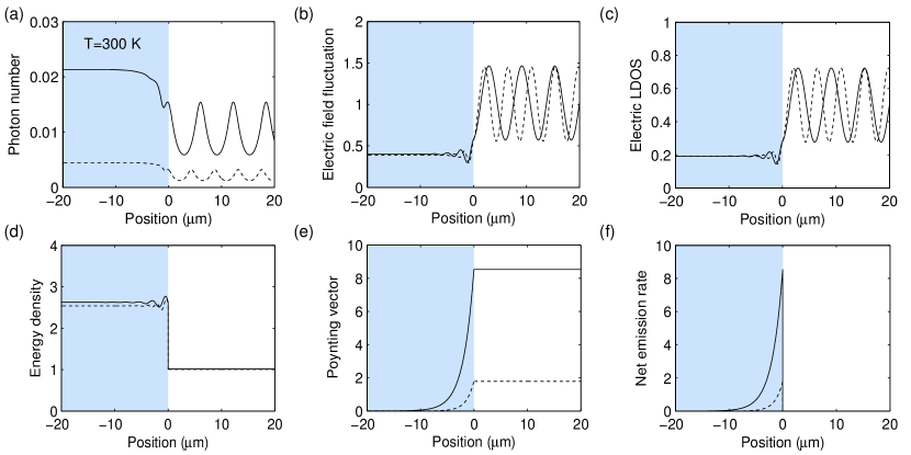
Figure 1: (Color online) (a) The effective photon number, (b) electric field fluctuation, (c) electric LDOS, (d) energy density, (e) Poynting vector, and (f) net emission rate in the vicinity of an interface separating a lossy medium with refractive index $n_{1}=2.5+0.5i$ and temperature 300 K from vacuum at 0 K. The solid lines correspond to the photon energy $\hbar\omega=0.10$ eV ($\lambda=12.4$ $\mu$m) and the dashed lines correspond to the photon energy $\hbar\omega=0.14$ eV ($\lambda=8.86$ $\mu$m). The electric field fluctuation is given in the units of $\hbar\omega/(2\pi\varepsilon_{0}cS)$, the electric LDOS in the units of $2/(\pi cS)$, the energy density in the units of $\hbar\omega/(2\pi cS)$, the Poynting vector in the units of $\hbar\omega/(1000\pi S)$, and the net emission rate in the units of $\hbar\omega^{2}/(1000\pi cS)$.

To investigate the physical implications of the concepts presented in Sec. II we compare the position-dependent photon number to the corresponding electric field fluctuation, electric LDOS, energy density, Poynting vector, and net emission rate in two geometries: a single interface separating a lossy medium from vacuum and a vacuum cavity formed between two lossy media. The definitions for the electric field fluctuation, energy density, electric LDOS, and Poynting vector coincide with the conventional Green’s function based definitions. Instead, the position-dependent photon-number operator predicts different results.

III.1 Dielectric-vacuum interface

The single interface structure consists of a semi-infinite lossy medium with refractive index $n=2.5+0.5i$ at temperature $T_{1}=300$ K. The field incident from vacuum is a vacuum field with $T_{2}=0$ K. Figure 1 shows the effective photon number, electric field fluctuation, electric LDOS, energy density, Poynting vector, and net emission rate as a function of position for the single interface geometry for photon energies $\hbar\omega=0.10$ eV and $\hbar\omega=0.14$ eV, corresponding to wavelengths $\lambda=12.4$ $\mu$m and $\lambda=8.86$ $\mu$m. The expectation value of the photon number operator in Eq. (20) is plotted in Fig. 1(a). The effective photon number has a strong position dependence and it oscillates both in the vacuum and inside the lossy medium. In the lossy medium the oscillations are damped and the photon number saturates to a constant value far from the interface. The damping takes place over a distance of 10 $\mu$m that approximately corresponds to the penetration depth of radiation. The oscillations in the vacuum can be explained by separately considering the interference of the field component terms generated by the lossy half-space and the incident field from the vacuum, i.e., the left and right source domain contributions $x^{\prime}\in]\!-\infty,0]$ and $x^{\prime}\in[0,\infty[$ in Eq. (20). On the vacuum side, the term $|G(x,\omega,x^{\prime})|^{2}$ in Eq. (20) is constant for the right source domain contribution as it describes a simple propagating wave in that region. The contribution from the left source domain involves a Green’s function with standing wave features and therefore $|G(x,\omega,x^{\prime})|^{2}$ for the left source domain oscillates. To preserve the canonical commutation relations, however, the oscillations are compensated by changes in the contribution of the fields generated by the lossy medium. This is a direct mathematical consequence imposed by the preservation of the canonical commutation relations and results in variations of the contributions of the vacuum field at $T_{2}=0$ K and the lossy layer at $T_{1}=300$ K as a function of position even in the vacuum. In lossy media, similar oscillations occur but they are quickly damped by the losses. The oscillations are expected to be related to defining the ladder operators so that they are proportional to the vector potential and the electric field. This implies that the resulting photon number is in fact a quantity that mainly reflects the features related to electric field and field–matter interactions involving electrical dipoles.

The corresponding position-dependent magnitude of the electric field fluctuation in Eq. (29) is plotted in Fig. 1(b). The magnitude in the vacuum is larger than inside the lossy medium. This is not always the case, since it depends on the refractive index of the medium and the source field temperature. The field fluctuations also exhibit similar oscillations as the photon numbers in Fig. 1(a) but the minima of the electric field fluctuations coincide with the maxima of the photon-number oscillations. In the lossy layer the fluctuations are quickly damped to a constant value. Overall, oscillations in the photon number are accompanied by the oscillations in the electric field fluctuations, but there is no direct correspondence between the two.

The electric LDOS in Eq. (31) is plotted in Fig. 1(c). The electric LDOS graphs clearly resemble the electric field fluctuations in Fig. 1(b) oscillating in the vacuum and saturating to constant values inside the lossy medium. In contrast to the field fluctutations, the electric LDOS is temperature independent and not directly proportional to the fluctuations. However, since the zero-point-field contribution dominates at chosen temperatures and frequencies, the oscillating photon number has only a small effect on the electric field fluctuations. The oscillations in the electric LDOS describe the modified emission rate due to interference better known as the Purcell effect in cavities.

The energy density in Eq. (28) is shown in Fig. 1(d). Inside the lossy medium, the energy density exhibits damped oscillations and in the vacuum it is perfectly constant since the electric and magnetic field contributions in the energy density are equal and out of phase so that the total energy density becomes constant. In the lossy medium the electric field contribution dominates in the energy density. This leads to oscillations that resemble the forms seen in the electric field fluctuation graphs in Fig. 1(b).

The Poynting vector in Eq. (27) is shown in Fig. 1(e). No net power propagates deep inside the lossy material since the absorption and emission of thermal photons is in balance, and therefore, the Poynting vector equals zero. The field generated in the material near the interface can propagate into the vacuum so that the Poynting vector grows exponentially and preserves its constant value through the vacuum indicating a constant radiative heat flow out of the lossy half-space.

The net emission rate given by Eq. (33) is plotted in Fig. 1(f). The net emission is naturally zero in the vacuum. The positive net emission in the lossy medium near the interface denotes that the rate of photon emission outweighs the rate of photon absorption. Inside the lossy medium the net emission rate decays to zero since the photon emission and absorption become balanced. However, no oscillations appear in the net emission rate. This is due to the infinitely large uniform half spaces and thermal field statistics. In the presence of a nonuniform temperature profile in the lossy medium (not shown) the oscillations seen in the electric LDOS in Fig. 1(c) are also present in the net emission rate in the lossy medium.

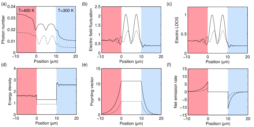
Figure 2: (Color online) (a) The effective photon number, (b) electric field fluctuation, (c) electric LDOS, (d) energy density, (e) Poynting vector, and (f) net emission rate in the vicinity of a vacuum gap separating lossy media with refractive indices $n_{1}=1.5+0.3i$ and $n_{2}=2.5+0.5i$ at temperatures 400 and 300 K. The width of the cavity is 10 $\mu$m. The solid lines correspond to the second resonant photon energy $\hbar\omega=0.118$ eV ($\lambda=10.5$ $\mu$m) and the dashed lines correspond to the off-resonant energy $\hbar\omega=0.140$ eV ($\lambda=8.86$ $\mu$m). The electric field fluctuation is given in the units of $\hbar\omega/(2\pi\varepsilon_{0}cS)$, the electric LDOS in the units of $2/(\pi cS)$, the energy density in the units of $\hbar\omega/(2\pi cS)$, the Poynting vector in the units of $\hbar\omega/(1000\pi S)$, and the net emission rate in the units of $\hbar\omega^{2}/(1000\pi cS)$.

III.2 Vacuum gap between lossy media

As a slightly more complex example we also investigate a cavity structure which consists of two semi-infinite media with refractive indices $n_{1}=1.5+0.3i$ and $n_{2}=2.5+0.5i$ at temperatures $T_{1}=400$ K and $T_{2}=300$ K, separated by a vacuum gap of thickness $10$ $\mu$m. Figure 2 shows the effective photon number, electric field fluctuation, electric LDOS, energy density, Poynting vector, and net emission rate as a function of position for the cavity geometry for photon energies $\hbar\omega=0.118$ eV ($\lambda=10.5$ $\mu$m) corresponding to the second resonance of the cavity and $\hbar\omega=0.140$ eV ($\lambda=8.86$ $\mu$m) that is off-resonant. As in the case of results for the single interface geometry presented above, there are periodic oscillations in the effective photon number as presented in Fig. 2(a). For the second resonant energy the photon number has two peaks in the cavity as expected. At resonant energies observing oscillations in the photon number, however, requires an asymmetric cavity: If the refractive indices of the left and right lossy media were equal (not shown), the photon-number oscillations inside the cavity would completely disappear for resonant frequencies. On the left and right of the cavity in Fig. 2(a), the photon number again saturates to constant values depending on the source field temperature.

The corresponding electric field fluctuations are presented in Fig. 2(b). As in the case of the single interface geometry, the magnitudes of the electric field fluctuations are larger in the vacuum than in the lossy medium. The extrema of the electric field fluctuations are located at the same positions as the extrema of the photon number in Fig. 2(a). Inside the lossy media, the oscillations are again damped and eventually reach constant values, which are different on the left and right due to the different source field temperatures.

The electric LDOS is plotted in Fig. 2(c). Again, the electric LDOS oscillates in the vacuum and saturates to constant values in the lossy media resembling the electric field fluctuation in Fig. 2(b). However, there are some differences. For example, the difference in the oscillation magnitudes of the resonant and off-resonant energies in the electric LDOS in the vacuum is larger than the corresponding difference in the electric field fluctuation in Fig. 2(b). This is due to the effect of the oscillating photon number in the electric field fluctuation. The effect is hardly visible in the electric field fluctuation in Fig. 2(b), but becomes larger when the temperature of the left medium is increased (not shown).

The energy density shown in Fig. 2(d) exhibits damped oscillations inside the lossy medium and in the vacuum it is perfectly constant as in the case of the single interface geometry. In the lossy media the energy density due to the electric field contribution is again larger than in the vacuum and leads to oscillations that resemble the form seen in the electric field fluctuation graph in Fig. 2(b). Note that the energy density is smaller in the left medium than in the right medium even though the left medium has a higher temperature. This is due to the effect of electric susceptibility which is larger at the right medium. However, if the temperature is increased on the left the energy density on the left at some point naturally exceeds the energy density on the right.

The Poynting vector is plotted in Fig. 2(e). In the vacuum gap, the Poynting vector is again constant since there is no dissipation. The positivity of the Poynting vector denotes net energy transfer towards the medium at lower temperature. Inside the lossy media, the Poynting vector asymptotically reaches zero far from the interfaces. The damping of the Poynting vector is faster in the right medium than in the left medium due to the larger imaginary part of the refractive index.

The net emission rate is shown in Fig. 2(f). Again the net emission rate is zero in the vacuum and it decays to zero inside the lossy media. Positive (negative) values denote that the rate of photon emission (absorption) outweighs the rate of photon absorption (emission). The higher absolute value of the net emission rate in the lossy medium with higher imaginary part of the refractive index is related to larger loss and the faster damping of the Poynting vector in Fig. 2(e). In the presence of small losses inside the cavity (not shown) the net emission rate exhibits oscillations similar to the oscillations of the electric LDOS in Fig. 2(c). This directly reflects the Purcell effect and position-dependent emission rate of particles placed in the cavity.

The proposed position-dependent ladder and photon-number operators predict that the effective photon numbers oscillate with respect to the positions as shown in Figs. 1(a) and 2(a). In contrast to the field quantities, the effective photon number provides a simple metric for finding the thermal balance formed due to interactions taking place through the electric field and electric dipoles as detailed in Eq. (33). Since the photon number as defined in this work is also expected to be directly related both to local temperature and rate of energy exchange taking place between the electric field and the dipoles constituting the lossy materials, we expect that the predicted photon-number oscillations can also be measured. A good candidate for such a measurement would be a setup consisting of a high-quality-factor cavity where the magnitude of oscillations as well as the incoming radiation on the left and right can be better controlled than in the single interface case. Photon-number measurements have already been performed in cavities Maître et al. (1997), but not in nonequilibrium conditions which is necessary for the oscillations of the effective photon number with respect to the position. If the cavity is asymmetric, the photon-number oscillations are more easily observable than in a symmetric cavity where the photon-number oscillations can disappear at resonant frequencies. If one had a thermometer that resonantly couples to one of the cavity resonances and is anisotropic so that it is capable of detecting only the single perpendicular mode studied in this work, then the predicted photon-number oscillations could be easily detected experimentally. In reality the measurement configuration is naturally more complex as controlling the directivity of a nanoscale thermometer may not be that straightforward, but similar effects are nevertheless also expected to be observable in fully three-dimensional configurations. As the taken approach is very general, generalizing the model to three dimensions is expected to be straightforward. In this paper we have investigated only thermal source fields in detail, but the introduced operators are expected to enable also a much more general description of the quantized fields obeying other kinds of quantum statistics. For example, replacing the noise operators with operators describing partly saturated emitters Häyrynen et al. (2010) could result in a simple but realistic quantum description of the generation of laser fields, and furthermore, the use of nonlinear source field operators Häyrynen et al. (2012, 2010) could even allow modeling single photon sources and detectors.

IV Conclusions

We have defined and studied position-dependent ladder operators for the electromagnetic field in a way that is consistent with the canonical commutation relations and also enables a physically meaningful definition of an effective position-dependent photon-number operator that has a very attractive and simple connection to the electric field, the temperature, and thermal balance of the system. The introduced operators predict oscillations in the expectation value of the effective photon number even in simple one-dimensional layered geometries. Since the effective photon number is expected to be directly related to experimentally observable local temperatures in measurements in which the field-matter interaction is dominated by the coupling to the electric field, this suggests that the oscillations could be experimentally observable by measuring similar oscillations in the temperature. This essentially differentiates our definition of the effective photon number from the conventional position-independent definitions that do not take the physical properties of the electric field similarly into account.

The introduced ladder and photon-number operators provide an additional means to quantify the electric field and give further insight into the local photon-number balance associated with the electric field and the formation of the local thermal equilibrium. The additional insight provided by the approach also allows improved understanding of the challenges and physical implications of separating the photon annihilation operator into parts emitted by the left and right source domains or left and right propagating parts as done in many seminal quantization schemes. If the requirement of canonical commutation relations and ease of physical interpretation are not relaxed, the separation is not generally possible. This is in agreement with the anomalies found in the commutation relations of the photon annihilation operator. However, possibly the greatest opportunities enabled by the new formulation and the consistent definitions of the ladder and photon-number operators are in extending the description to quantum systems that are not limited to thermal fields. This could, e.g., enable a more versatile description of the noise and measurement backaction in complex and realistic quantum systems.

*

Appendix A Green’s functions

A.1 Single interface

The single interface geometry consists of media with refractive indices $n_{1}$ ($x<0$) and $n_{2}$ ($x>0$). The corresponding wave vectors are $k_{1}$ and $k_{2}$. The Green’s function for the single interface geometry is given in the left half-space ($x<0$) by Matloob and Loudon (1996)

$$G_{\{x<0\}}(x,\omega,x^{\prime})=\; \frac{i\,\theta(-x^{\prime})}{2k_{1}}\Big{(}e^{ik_{1}|x-x^{\prime}|}+re^{-ik_{1}(x+x^{\prime})}\Big{)}$$

$$+\frac{i\,\theta(x^{\prime})}{2k_{2}}t^{\prime}e^{-i(k_{1}x-k_{2}x^{\prime})}$$ (34)

and on the right half-space ($x>0$) by

$$G_{\{x>0\}}(x,\omega,x^{\prime})=\; \frac{i\,\theta(-x^{\prime})}{2k_{1}}te^{i(k_{2}x-k_{1}x^{\prime})}$$

$$+\frac{i\,\theta(x^{\prime})}{2k_{2}}\Big{(}e^{ik_{2}|x-x^{\prime}|}+r^{\prime}e^{ik_{2}(x+x^{\prime})}\Big{)},$$ (35)

where $\theta(x)$ is the step function and $r$ and $t$ are the Fresnel coefficients for reflection and transmission on the left given for normal incidence by

$$r=\frac{n_{1}-n_{2}}{n_{1}+n_{2}},\hskip 14.22636ptt=\frac{2n_{1}}{n_{1}+n_{2}}.$$ (36)

The reflection and transmission coefficients on the right $r^{\prime}$ and $t^{\prime}$ are obtained by switching the indices 1 and 2 in the expressions of $r$ and $t$.

In the Green’s functions of both half-spaces in Eqs. (34) and (35), the first term describes the field generated by the source point in the left half-space and the second term describes the field generated by the source point in the right half-space.

A.2 Two interfaces

The slab geometry consists of media with refractive indices $n_{1}$ ($x<0$), $n_{2}$ ($0<x<d$), and $n_{3}$ ($x>d$). The corresponding wave vectors are $k_{1}$, $k_{2}$, and $k_{3}$. The Green’s function for the slab geometry is given in the left medium ($x<0$) by Matloob and Loudon (1996)

$$G_{\{x<0\}}(x,\omega,x^{\prime})$$

$$=\; \frac{i\,\theta(-x^{\prime})}{2k_{1}}\Big{(}e^{ik_{1}|x-x^{\prime}|}+\mathcal{R}_{1}e^{-ik_{1}(x+x^{\prime})}\Big{)}$$

$$+\frac{i\,[\theta(x^{\prime})-\theta(x^{\prime}-d)]}{2k_{2}}\mathcal{T}_{1}^{\prime}e^{-ik_{1}x}\Big{(}e^{ik_{2}x^{\prime}}$$

$$+\nu\mathcal{R}_{2}[e^{-ik_{2}(x^{\prime}-2d)}+\mathcal{R}_{1}^{\prime}e^{ik_{2}(x^{\prime}+2d)}]\Big{)}$$

$$+\frac{i\,\theta(x^{\prime}-d)}{2k_{3}}\mathcal{T}_{2}^{\prime}\mathcal{T}_{1}^{\prime}e^{-i[k_{1}x-k_{2}d-k_{3}(x^{\prime}-d)]}.$$ (37)

The first term describes the field generated by the left half-space, the second term corresponds to the field generated by the medium within the interfaces, and the last term corresponds to the field generated by the right half-space. In our notation $\mathcal{R}_{1}$, $\mathcal{R}_{2}$, $\mathcal{T}_{1}$, and $\mathcal{T}_{2}$ are the reflection and transmission coefficients for the first and second interfaces of the two-interface structure. They are given in terms of the single interface Fresnel coefficients in Eq. (36) as

$$\mathcal{R}_{1} =\frac{r_{1}+r_{2}e^{2ik_{2}d}}{1+r_{1}r_{2}e^{2ik_{2}d}},\hskip 14.22636pt\mathcal{R}_{2}=r_{2},$$ (38)

$$\mathcal{T}_{1} =\frac{t_{1}}{1+r_{1}r_{2}e^{2ik_{2}d}},\hskip 14.22636pt\mathcal{T}_{2}=t_{2}.$$ (39)

The parameter $\nu$ in the Green’s function is expressed as

$$\nu=\frac{1}{1+r_{1}r_{2}e^{2ik_{2}d}}.$$ (40)

The Green’s function in the right medium ($x>d$) is, respectively, given by Matloob and Loudon (1996)

$$G_{\{x>d\}}(x,\omega,x^{\prime})$$

$$=\; \frac{i\,\theta(-x^{\prime})}{2k_{1}}\mathcal{T}_{1}\mathcal{T}_{2}e^{i[k_{3}(x-d)+k_{2}d-k_{1}x^{\prime}]}$$

$$+\frac{i\,[\theta(x^{\prime})-\theta(x^{\prime}-d)]}{2k_{2}}\mathcal{T}_{2}e^{ik_{3}(x-d)}\Big{(}e^{ik_{2}(d-x^{\prime})}$$

$$+\nu\mathcal{R}_{1}^{\prime}[e^{ik_{2}(x^{\prime}+d)}+\mathcal{R}_{2}e^{ik_{2}(3d-x^{\prime})}]\Big{)}$$

$$+\frac{i\,\theta(x^{\prime}-d)}{2k_{3}}\Big{(}e^{ik_{3}|x-x^{\prime}|}+\mathcal{R}_{2}^{\prime}e^{ik_{3}(x+x^{\prime}-2d)}\Big{)}.$$ (41)

and inside the cavity ($0<x<d$), the Green’s function is expressed as

$$G_{\{0<x<d\}}(x,\omega,x^{\prime})$$

$$=\; \frac{i\,\theta(-x^{\prime})}{2k_{1}}\mathcal{T}_{1}\Big{(}e^{i(k_{2}x-k_{1}x^{\prime})}+\mathcal{R}_{2}e^{-i[k_{2}(x-2d)+k_{1}x^{\prime}]}\Big{)}$$

$$+\frac{i\,[\theta(x^{\prime})-\theta(x^{\prime}-d)]}{2k_{2}}\Big{(}e^{ik_{2}|x-x^{\prime}|}$$

$$+\nu\mathcal{R}_{2}[e^{-ik_{2}(x+x^{\prime}-2d)}+\mathcal{R}_{1}^{\prime}e^{-ik_{2}(x-x^{\prime}-2d)}]$$

$$+\nu\mathcal{R}_{1}^{\prime}[e^{ik_{2}(x+x^{\prime})}+\mathcal{R}_{2}e^{ik_{2}(x-x^{\prime}+2d)}]\Big{)}$$

$$+\frac{i\,\theta(x^{\prime}-d)}{2k_{3}}\mathcal{T}_{2}^{\prime}\Big{(}e^{-i[k_{2}(x-d)-k_{3}(x^{\prime}-d)]}$$

$$+\mathcal{R}_{1}^{\prime}e^{i[k_{2}(x+d)+k_{3}(x^{\prime}-d)]}\Big{)}.$$ (42)

Again, the three different terms describe the fields generated by different source domains.

References

- Sorger and Zhang (2011) V. J. Sorger and X. Zhang, Science 333, 709 (2011).
- Oulton et al. (2009) R. F. Oulton, V. J. Sorger, R. Zentgraf, R.-M. Ma, C. Gladden, L. Dai, G. Bartal, and X. Zhang, Nature 461, 629 (2009).
- Huang et al. (2013) L. Huang, X. Chen, H. Mühlenbernd, H. Zhang, S. Chen, B. Bai, Q. Tan, G. Jin, K.-W. Cheah, C.-W. Qiu, J. Li, T. Zentgraf, and S. Zhang, Nat. Commun. 4, 2808 (2013).
- Sadi et al. (2013) T. Sadi, J. Oksanen, J. Tulkki, P. Mattila, and J. Bellessa, IEEE J. Sel. Top Quantum Electron. 19, 1 (2013).
- Taubner et al. (2006) T. Taubner, D. Korobkin, Y. Urzhumov, G. Shvets, and R. Hillenbrand, Science 313, 1595 (2006).
- Hillenbrand et al. (2002) R. Hillenbrand, T. Taubner, and F. Keilmann, Nature 418, 159 (2002).
- Nakamura and Krames (2013) S. Nakamura and M. Krames, Proceedings of the IEEE 101, 2211 (2013).
- Heikkilä et al. (2013) O. Heikkilä, J. Oksanen, and J. Tulkki, Appl. Phys. Lett. 102, 111111 (2013).
- Russell (2003) P. Russell, Science 299, 358 (2003).
- Akahane et al. (2003) Y. Akahane, T. Asano, B. S. Song, and S. Noda, Nature 425, 944 (2003).
- Tanaka et al. (2010) K. Tanaka, E. Plum, J. Y. Ou, T. Uchino, and N. I. Zheludev, Phys. Rev. Lett. 105, 227403 (2010).
- Mattiucci et al. (2013) N. Mattiucci, M. J. Bloemer, N. Aközbek, and G. D’Aguanno, Sci. Rep. 3, 3203 (2013).
- Zavatta et al. (2011) A. Zavatta, J. Fiurášek, and M. Bellini, Nature Photonics 5, 52 (2011).
- Ferreyrol et al. (2010) F. Ferreyrol, M. Barbieri, R. Blandino, S. Fossier, R. Tualle-Brouri, and P. Grangier, Phys. Rev. Lett. 104, 123603 (2010).
- Partanen et al. (2012) M. Partanen, T. Häyrynen, J. Oksanen, and J. Tulkki, Phys. Rev. A 86, 063804 (2012).
- Gröblacher et al. (2009) S. Gröblacher, K. Hammerer, M. R. Vanner, and M. Aspelmeyer, Nature 460, 724 (2009).
- Collette et al. (2013) M. Collette, N. Beaudoin, and S. Gauvin, Proc. SPIE 8772, 87721D (2013).
- Häyrynen et al. (2011) T. Häyrynen, J. Oksanen, and J. Tulkki, Phys. Rev. A 83, 013801 (2011).
- Häyrynen et al. (2009) T. Häyrynen, J. Oksanen, and J. Tulkki, J. Phys. B 42, 145506 (2009).
- Knöll et al. (1987) L. Knöll, W. Vogel, and D. G. Welsch, Phys. Rev. A 36, 3803 (1987).
- Knöll et al. (1991) L. Knöll, W. Vogel, and D.-G. Welsch, Phys. Rev. A 43, 543 (1991).
- Allen and Stenholm (1992) L. Allen and S. Stenholm, Opt. Commun. 93, 253 (1992).
- Huttner and Barnett (1992) B. Huttner and S. M. Barnett, Phys. Rev. A 46, 4306 (1992).
- Barnett and Loudon (1995) R. Barnett, S. M. Matloob and R. Loudon, J. Mod. Opt. 42, 1165 (1995).
- Matloob et al. (1995) R. Matloob, R. Loudon, S. M. Barnett, and J. Jeffers, Phys. Rev. A 52, 4823 (1995).
- Matloob and Loudon (1996) R. Matloob and R. Loudon, Phys. Rev. A 53, 4567 (1996).
- Raymer and McKinstrie (2013) M. G. Raymer and C. J. McKinstrie, Phys. Rev. A 88, 043819 (2013).
- Barnett et al. (1996) S. M. Barnett, C. R. Gilson, B. Huttner, and N. Imoto, Phys. Rev. Lett. 77, 1739 (1996).
- Ueda and Imoto (1994) M. Ueda and N. Imoto, Phys. Rev. A 50, 89 (1994).
- Aiello (2000) A. Aiello, Phys. Rev. A 62, 063813 (2000).
- Di Stefano et al. (2000) O. Di Stefano, S. Savasta, and R. Girlanda, Phys. Rev. A 61, 023803 (2000).
- Novotny and Hecht (2006) L. Novotny and B. Hecht, Principles of nano-optics (Cambridge University Press, Cambridge, 2006).
- Scheel et al. (1998) S. Scheel, L. Knöll, and D.-G. Welsch, Phys. Rev. A 58, 700 (1998).
- Gruner and Welsch (1996) T. Gruner and D.-G. Welsch, Phys. Rev. A 54, 1661 (1996).
- Dung et al. (1998) H. T. Dung, L. Knöll, and D.-G. Welsch, Phys. Rev. A 57, 3931 (1998).
- Janowicz et al. (2003) M. Janowicz, D. Reddig, and M. Holthaus, Phys. Rev. A 68, 043823 (2003).
- Loudon (2000) R. Loudon, The quantum theory of light (Oxford University Press, Oxford, 2000).
- Ziolkowski (2001) R. W. Ziolkowski, Phys. Rev. E 63, 046604 (2001).
- Ruppin (2002) R. Ruppin, Phys. Lett. A 299, 309 (2002).
- Vorobyev (2012) O. B. Vorobyev, Prog. Electromagn. Res. B 40, 343 (2012).
- Vorobyev (2013) O. B. Vorobyev, J. Mod. Opt. 60, 1253 (2013).
- Joulain et al. (2003) K. Joulain, R. Carminati, J.-P. Mulet, and J.-J. Greffet, Phys. Rev. B 68, 245405 (2003).
- Jackson (1999) J. D. Jackson, Classical electrodynamics (Wiley, New York, 1999).
- Büttiker (1992) M. Büttiker, Phys. Rev. B 46, 12485 (1992).
- Sääskilahti et al. (2013) K. Sääskilahti, J. Oksanen, and J. Tulkki, Phys. Rev. E 88, 012128 (2013).
- Bohren and Huffman (1998) C. F. Bohren and D. R. Huffman, Absorption and scattering of light by small particles (Wiley, Chichester, UK, 1998).
- Maître et al. (1997) X. Maître, E. Hagley, G. Nogues, C. Wunderlich, P. Goy, M. Brune, J. M. Raimond, and S. Haroche, Phys. Rev. Lett. 79, 769 (1997).
- Häyrynen et al. (2010) T. Häyrynen, J. Oksanen, and J. Tulkki, Phys. Rev. A 81, 063804 (2010).
- Häyrynen et al. (2012) T. Häyrynen, J. Oksanen, and J. Tulkki, Europhys. Lett. 100, 54001 (2012).
- Häyrynen et al. (2010) T. Häyrynen, J. Oksanen, and J. Tulkki, Eur. Phys. J. D 56, 113 (2010).