Retention capacity of correlated surfaces

Abstract

We extend the water retention model [C. L. Knecht et al., Phys. Rev. Lett. 108, 045703 (2012)] to correlated random surfaces. We find that the retention capacity of discrete random landscapes is strongly affected by spatial correlations among the heights. This phenomenon is related to the emergence of power-law scaling in the lake volume distribution. We also solve the uncorrelated case exactly for a small lattice and present bounds on the retention of uncorrelated landscapes.

I Introduction

Consider the discrete landscape in Fig. 1: If water rains on this landscape and is allowed to flow out through its open boundaries, one may ask what is the volume of water retained by the landscape, i.e., when the water level of all ponds has reached its maximum. Recently, Knecht et al. investigated this question for random landscapes with uncorrelated heights, coining the term water retention model Knecht et al. (2012). Further studies of the critical behavior of the water retention model have also been reported by Baek and Kim Baek and Kim (2012). An example of a correlated landscape, where all ponds and lakes are at their maximum capacity, is shown in Fig. 2. Looking at the examples in Figs. 1 and 2, one anticipates that the degree of correlation among the heights of the landscapes can drastically impact on their retention behavior. This subject is studied in the present work.

There has been recently much interest in the properties of random landscapes, with and without spatial correlations Kondev and Henley (1995); Kondev et al. (2000); Majumdar and Martin (2006); Schrenk et al. (2012, 2013). Such landscapes are used on different scales, from deposition phenomena Barabási and Stanley (1995) to driven movement and transport in random geometries Araújo et al. (2002); Le Doussal and Wiese (2009), geomorphology Xu et al. (1993); Czirók et al. (1993); Pastor-Satorras and Rothman (1998); Nikora et al. (1999), and city growth Makse et al. (1998). Related concepts have also been generalized to non-Euclidean graphs and their partitioning Carmi et al. (2008); Sollich et al. (2008).

The water retention capacity is a global property of a random landscape. A closely related question is how to predict through which part of the boundary the water of spilling ponds will flow out of the landscape. Ponds spilling to different parts of the boundary are separated by watersheds of the considered landscape Fehr et al. (2011a); Daryaei et al. (2012) and share statistical properties of optimum paths and polymers in strongly disordered media Andrade Jr. et al. (2011). For uncorrelated random heights, watersheds are known to be fractals of dimension ${1.2168\pm 0.0005}$ Fehr et al. (2012). This fractal dimension is affected by long-range correlations in the landscape Fehr et al. (2011b).

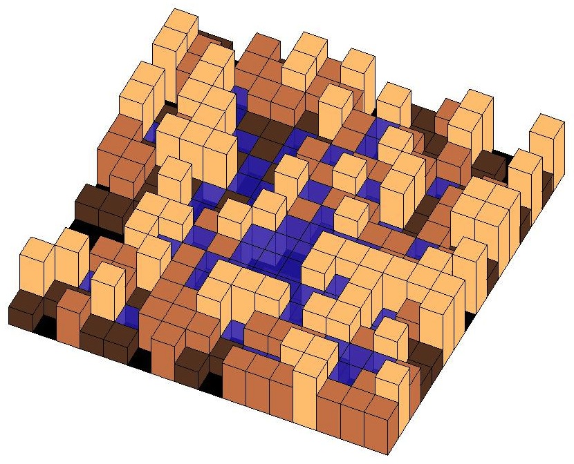
Figure 1: (Color online) Snapshot of the water retention model on a square lattice of size ${16\times 16}$, with number of levels ${n=4}$. The colors of the cubes indicate the landscape height, which varies from zero (black) to ${n-1=3}$ (light orange, light gray). The retention capacity of this landscape is $72$ (lattice units). Blue (dark gray) transparent squares indicate the surfaces of lakes of retained water.

Here we report that the retention capacity of random landscapes is strongly affected by long-range height correlations. This adds to the understanding of this recently introduced model Knecht et al. (2012), because natural landscapes are typically characterized by such correlations Xu et al. (1993); Czirók et al. (1993); Pastor-Satorras and Rothman (1998); Nikora et al. (1999) and the two previous studies of the model dealt only with uncorrelated heights Knecht et al. (2012); Baek and Kim (2012). We find that the decomposition property of the retention is valid for the correlated case as well. In addition, we report new derivations of an exact result and some bounds for the uncorrelated case.

For the numerical and analytical treatment of the water retention problem, we use its analogies to percolation Stauffer and Aharony (1994). In particular, we use an algorithm based on invasion percolation Wilkinson and Willemsen (1983), and we interpret our results establishing connections to percolation with correlated disorder Weinrib (1984); Prakash et al. (1992); Schmittbuhl et al. (1993); Mandre and Kalda (2011); Schrenk et al. (2013) and on rough surfaces Schmittbuhl et al. (1993); Kondev and Henley (1995); Olami and Zeitak (1996).

The remainder of this article is structured as follows. Section II discusses the water retention model on uncorrelated random landscapes. The model is solved exactly for a small lattice in Sec. A. The impact of height correlations on the retention is analyzed in Sec. III. Conclusions are drawn in Sec. IV.

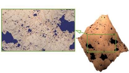
Figure 2: (Color online) Retention model with continuous heights on a lattice of size $512\times 512$. Surfaces of lakes are indicated in blue. The Hurst exponent is ${H=0.75}$, see e.g. Refs. Saupe (1988); Makse et al. (1996); Ballesteros and Parisi (1999); Kondev et al. (2000); Ahrens and Hartmann (2011) for details.

II Water retention model

We recall the original definition of the water retention model, as introduced in Ref. Knecht et al. (2012), along with some first results. Consider a square lattice of length $L$, consisting of ${N=L^{2}}$ sites, with free boundary conditions. Each site of the lattice, covering a unitary area, can be seen as the base of a square column with a certain height. The set of all $N$ square columns makes up a discrete landscape (see Fig. 1 and e.g. Refs. Kondev et al. (2000); Knecht et al. (2012); Schrenk et al. (2012)). In the original water retention model, we assume that the heights of the columns are integers in the interval ${[0,n-1]}$, where $n$ is the number of levels, a parameter of the landscape. For simplicity, all $n$ heights appear with the same probability $1/n$.

To determine the volume of water retained by a given landscape, it is convenient to use the invasion algorithm of Ref. Knecht et al. (2012). There, the landscape is invaded, similarly to invasion percolation Wilkinson and Willemsen (1983), starting from its boundaries. The water level at which a site is first invaded, minus the terrain height at this site, gives the maximum retained volume at that site.

Given an ensemble of landscapes, of size $L$ with $n$ levels, one can define the average volume ${R_{n}^{(L)}}$ of retained water. First we consider uncorrelated landscapes as in Ref. Knecht et al. (2012); Baek and Kim (2012), to illustrate the model. Figures 3 and 4 show the retention ${R_{n}^{(L)}}$ for landscapes with equal probability for each of the $n$ heights as function of the lattice size $L$. In Fig. 4, ${R_{n}^{(L)}}$ is divided by $L^{2}$ to show that the retention is proportional to $L^{2}$ for large lattice sizes $L$. As reported in Ref. Knecht et al. (2012), the retention of a landscape of size $L$ is not always monotonically increasing with the number of levels $n$: For example, one observes in the inset of Fig. 3 that the curves for ${R_{2}^{(L)}}$ and ${R_{3}^{(L)}}$ intersect for ${L=51.2\pm 0.1}$ Knecht et al. (2012). This can also be observed in Fig. 4, where for small $L$ the retention grows monotonically in $n$, while for large $L$ this is not always the case, as can be observed for large system sizes for $n=2,3$; $4,5$; and $7,8$ Knecht et al. (2012). It was argued in Ref. Knecht et al. (2012) that the retention ${R_{n}^{(L)}}$ of such $n$-level landscapes can be expressed as a sum of terms ${R_{2}^{(L)}(p)}$ for two-level landscapes with probability $p$ that a site has height $0$ and probability ${1-p}$ that it has height $1$:

$$R_{n}^{(L)}=\sum_{i=1}^{n-1}R_{2}^{(L)}(i/n).$$ (1)

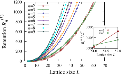
Figure 3: (Color online) Main plot: Retention $R_{n}^{(L)}$ of an $n$-level system of size $L^{2}$ as function of $L$. Results are averages over at least $10^{4}$ samples. Inset: Data for 2 and 3 levels, showing their crossing behavior. Random numbers have been generated with the algorithms of Refs. Ziff (1998); Matsumoto and Nishimura (1998).

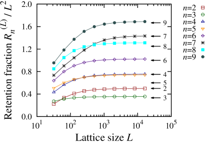
Figure 4: (Color online) Retention per site ${R_{n}^{(L)}/L^{2}}$ of an $n$-level system of size $L^{2}$ as function of $L$. The arrows indicate the lower bounds on ${R_{n}^{(L)}/L^{2}}$, for $n$ levels and large $L$, given by Eq. (5), with ${p_{c}=0.59274602}$ Ziff (2011).

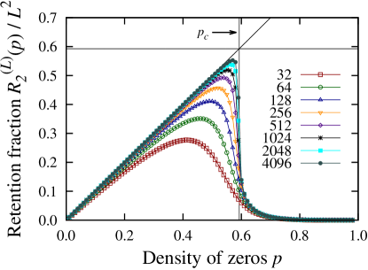
Figure 5: (Color online) Retention fraction ${R_{2}^{(L)}/L^{2}}$ as function of the density of zeros $p$ in the landscape for different $L$. The horizontal line indicates the site percolation threshold, ${p_{c}=0.59274602}$ Ziff (2011). The other straight solid line is the plot of ${f(p)=p}$.

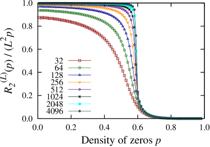
Figure 6: (Color online) ${R_{2}^{(L)}/(L^{2}p)}$ as function of the density of zeros $p$ in the landscape.

Figures 5 and 6 show that, for ${n=2}$ levels, the retention fraction ${R_{2}^{(L)}(p)/L^{2}}$, for large $L$, approaches $p$ for $p$ below the site percolation threshold $p_{c}$ (of the square lattice) and decreases to zero after reaching ${{R_{2}^{(L)}(p_{c})}=p_{c}}$. This behavior can be explained by considering

$$r_{2}(p)=\lim_{L\to\infty}R_{2}^{(L)}(p)/L^{2},$$ (2)

the retention fraction of the two-level landscape in the thermodynamic limit, ${L\to\infty}$: Each site of height zero that is not part of the percolating cluster, containing a fraction $P_{\infty}(p)$ of sites, retains one unit volume of water Knecht et al. (2012), such that

$$r_{2}(p)=p-P_{\infty}(p).$$ (3)

Analyzing the retention in the limits of large and small lattice size $L$ helps understanding why some retention curves show crossings. We focus first on the behavior of the retention fraction $R_{n}^{(L)}/L^{2}$ for large $L$, seen in Fig. 4 (the case ${L=3}$ is solved exactly in Appendix A). It is useful to find lower and upper bounds on

$$r_{n}=\lim_{L\to\infty}R_{n}^{(L)}/L^{2}.$$ (4)

Using Eqs. (1) and (3), Knecht et al. give an approximate expression for $r_{n}$ Knecht et al. (2012): This is a lower bound since, for $L\to\infty$, from Eq. (3), $r_{2}(p)\geq p\theta(p_{c}-p)$, such that

$$r_{n}=\sum_{i=1}^{n-1}r_{2}\left(\frac{i}{n}\right)\geq\sum_{i=1}^{n-1}\frac{i}{n}\theta(p_{c}-i/n)=\frac{n^{*}(n^{*}+1)}{2n},$$ (5)

where $n^{*}=\left\lfloor{np_{c}}\right\rfloor$ is the truncated integer part of $np_{c}$ and $\theta(x)$ is the Heaviside step function, defined as

$$\theta(x)=\left\{\begin{array}[]{ll}0&\mbox{if }x<0\\ 1&\mbox{if }x\geq 0\end{array}\right..$$ (6)

Figure 4 shows that the bound in Eq. (5), indicated by the black arrows on the right-hand side, is consistent with the numerical data and in agreement with the observed crossing behavior for the considered range of $n$. Without using the decomposition formula in Eq. (1), one obtains an upper bound on $r_{n}$ by considering the maximum amount of water that can be retained on a landscape of sufficiently large $L$: Suppose that $L$ is such that $L^{2}/n\gtrsim 4(L-1)$. This is enough to ensure that all sites in the boundary of the lattice can be occupied with square columns of the maximum height ${n-1}$. Since all columns of height smaller than ${n-1}$ are placed in the interior of such a landscape, it retains at most a volume of ${(n-1)L^{2}/2}$. Dividing by the number of sites $L^{2}$ and taking the limit $L\to\infty$ gives:

$$r_{n}\leq(n-1)/2.$$ (7)

We note that while the lower bound in Eq. (5) corresponds to approximating the curve of $r_{2}(p)$ by a step function which is zero for ${p>p_{c}}$, the upper bound in Eq. (7) is the same that one would obtain by using ${r_{2}(p)\leq p}$, for ${0\leq p\leq 1}$ combined with the decomposition formula in Eq. (1). Therefore, since ${p_{c}>1/2}$ Riordan and Walters (2007); Ziff (2011); Jacobsen (2014), for ${n=2}$ the upper and lower bounds coincide, and ${r_{2}=1/2}$ is the exact solution (see Fig. 4 and also Fig. 8). Basically, for a two-level system, the clusters of zeros are sub-critical and they become all filled with the water, which sits on exactly half of the sites. Here, we are assuming $L\to\infty$ so there are no finite-size effects.

We also note that one can use the results in Eq. (5), see Refs. Knecht et al. (2012); Baek and Kim (2012), and Eq. (7) to obtain bounds on the continuum version of the retention model, i.e., the case where the number of levels $n$ becomes infinite. Dividing the retention per site $r_{n}$ by $n$, one finds for this limit:

$$p_{c}^{2}/2\leq\lim_{n\to\infty}r_{n}/n\leq 1/2,$$ (8)

which is in agreement with the numerical result ${0.1820\pm 0.0002}$ Knecht et al. (2012) and our simulations (not shown) of the continuum model (we note that $p_{c}^{2}/2\approx 0.17567$).

III Impact of correlations

(a) $H=-1$	(b) $H=-0.5$
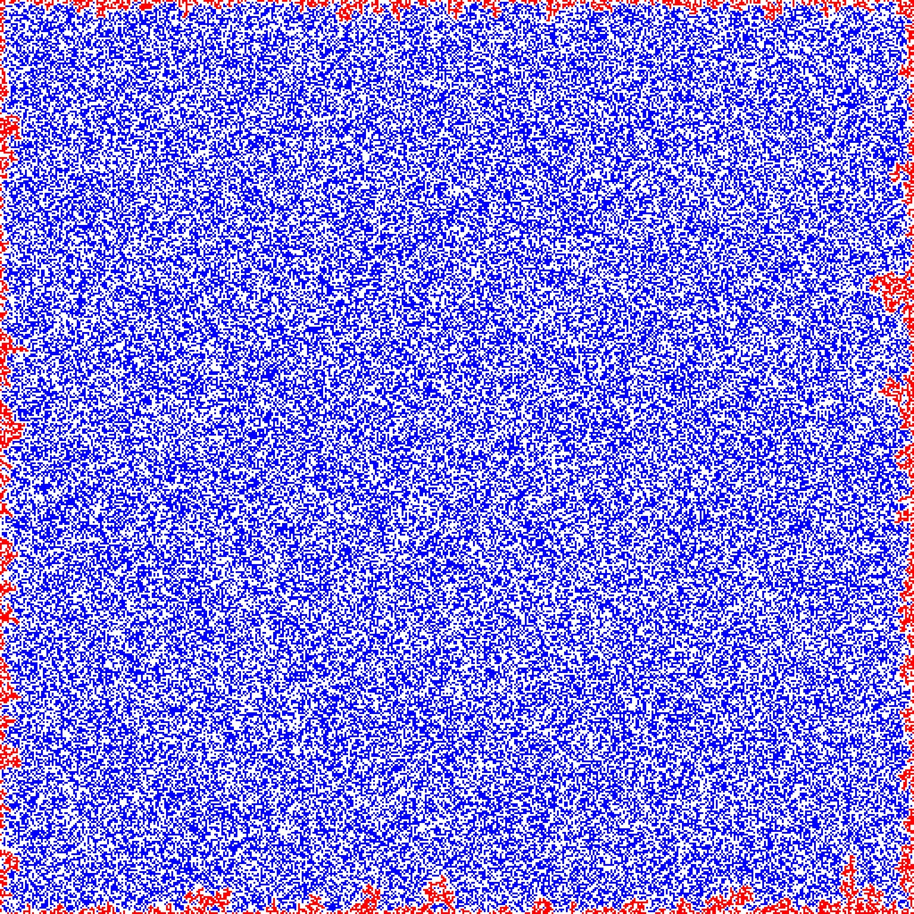
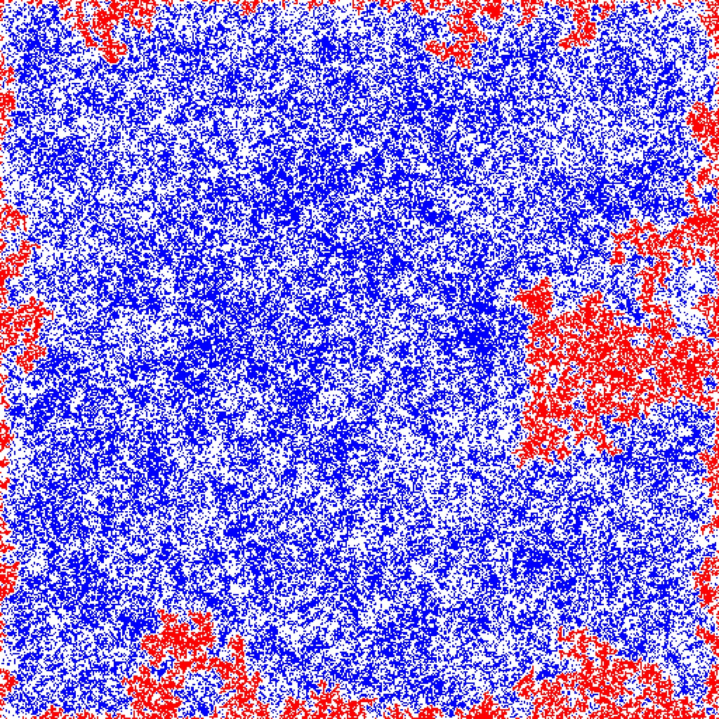
(c) $H=0$	(d) $H=0.5$

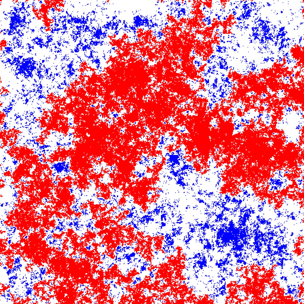
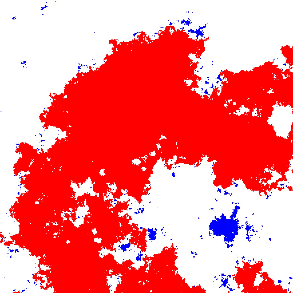
Figure 7: (Color online) Snapshots of the water retention model with $n=2$ levels. One half of the sites has height $1$, shown as white squares, and the other half has height $0$. The sites with height $0$ are colored in blue (dark gray) if they retain water, and they are colored in red (light gray) otherwise (draining to the boundary). $H$ increases from (a) to (d) and the lattice size is $L=512$. For $H=0$, it is known that the boundaries of the lakes are fractal with dimension $3/2$ Kondev and Henley (1995); Kondev et al. (2000); Schrenk et al. (2013), which corresponds to a Gaussian free field or $\text{SLE}_{4}$ Schramm and Sheffield (2009). Furthermore, for $0\leq H\leq 1$, it is believed that the boundary fractal dimension is $(3-H)/2$ Kondev and Henley (1995); Kondev et al. (2000); Schwartz (2001).

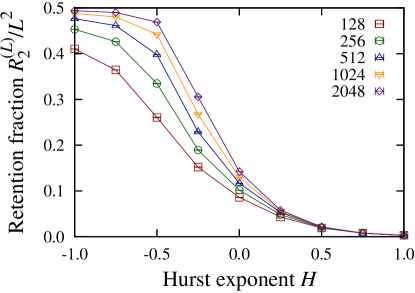
Figure 8: (Color online) Retention fraction $R_{2}^{(L)}/L^{2}$ for ${n=2}$ levels as function of the Hurst exponent $H$ for different lattice sizes $L$.

So far, we have considered landscapes with uncorrelated heights. However, the reason why the landscape in Fig. 2 looks natural is that its heights are spatially correlated. To analyze the impact of long-range correlations of the heights on the retention capacity, it is convenient to consider the canonical version of the model. There, every height appears exactly $N/n$ times (“canonical”), rather than with probability $1/n$ (“grand canonical”) Newman and Ziff (2000, 2001); Knecht et al. (2012); Hu et al. (2012). As discussed in Ref. Knecht et al. (2012), this does not significantly affect the behavior of the model. Our correlated landscapes are obtained in the following from the Fourier filtering method with Hurst exponent $H$, corresponding to a power spectrum $S(\mathbf{f})$ of the heights scaling as $S(\mathbf{f})\sim|\mathbf{f}|^{-2(H+1)}$, for low frequencies $|\mathbf{f}|$, see e.g. Refs. Saupe (1988); Makse et al. (1996); Ballesteros and Parisi (1999); Kondev et al. (2000); Ahrens and Hartmann (2011). Empirically, it has been observed that natural landscapes can be described by $H$ in the range of ${0.3\lesssim H\lesssim 0.95}$ Xu et al. (1993); Czirók et al. (1993); Pastor-Satorras and Rothman (1998); Nikora et al. (1999).

To discretize a random landscape into $n$ levels of height $0$ to ${n-1}$, it is convenient to consider the concept of ranked surfaces Schrenk et al. (2012). The recipe to discretize the continuous landscape is as follows: First, the ranked surface corresponding to the given landscape is obtained by ranking the sites according to the landscape heights. Then, one follows the rank of sites, starting from the lowest one, and assigns height $0$ to the first $N/n$ sites. The next $N/n$ sites in the ranking are assigned height $1$, and so on, until the highest sites have been assigned height $n-1$. This procedure gives landscapes like the ones in the canonical retention model. Therefore, discretizing an uncorrelated landscape, e.g. with uniformly and randomly distributed heights, or with $H=-1$, recovers the canonical version, as introduced in Ref. Knecht et al. (2012). Here we require that the number of sites can be divided by the number of levels $n$ such that there is no remainder, $L^{2}\,\text{mod}\,n=0$. This restricts the possible combinations of $L$ and $n$.

Figure 7 shows snapshots of the model for ${n=2}$ levels and different values of $H$. Retained water is shown in blue while water draining to the boundaries is shown in red. From these typical configurations, qualitatively speaking, one expects that the mean retention decreases with increasing $H$. This is confirmed by the data in Fig. 8, where the retention fraction $R_{2}^{(L)}/L^{2}$ is shown as function of $H$. By measuring the retention of two-level systems with variable fraction $p$ of sites with height zero $R_{2}^{(L)}(p)$ (not shown) and comparing this to direct measurements of $R_{n}^{(L)}$ for $n$-level systems, we confirmed that, within error bars, the decomposition formula in Eq. (1) is also valid for ${H>-1}$.

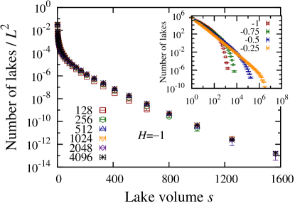
Figure 9: (Color online) Uncorrelated regime and evolution with $H$. Main plot: Number of lakes of size $s$ per site as function of $s$ with ${H=-1}$ and for different lattice sizes $L$. Inset: Evolution of the lake size distribution with $H$, for fixed ${L=4096}$. The sites have height $0$ or $1$ with equal probability $1/2$. Results are averages over $10^{4}$ samples.

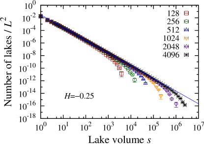
Figure 10: (Color online) Correlated percolation regime. Number of lakes per site for ${H=-0.25}$ and different lattice sizes $L$. The solid blue line is a guide to the eye with slope $-2.02$.

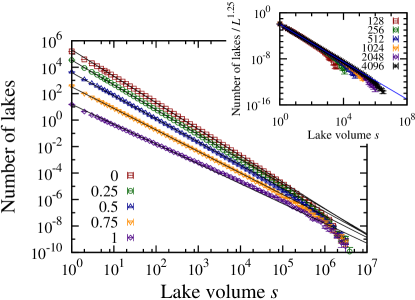
Figure 11: (Color online) Main plot: Number of lakes as function of the lake volume for different non-negative $H$ and ${L=4096}$. Straight black lines are guides to the eye with slope ${2-H/2}$ Kondev and Henley (1995); Olami and Zeitak (1996); Kondev et al. (2000). Inset: Number of lakes, rescaled by ${L^{2-H}=L^{1.25}}$ Olami and Zeitak (1996), as function of the lake volume, for ${H=0.75}$ and different lattice sizes $L$. The solid blue line is a guide to the eye with slope ${2-H/2=1.625}$ Olami and Zeitak (1996); Kondev and Henley (1995); Kondev et al. (2000).

Looking at the images in Figs. 2 and 7, one anticipates that, for correlated landscapes, the lake volumes vary considerably, while in the uncorrelated case, the lake sizes are more homogeneous. To quantify this observation, we measure the number of lakes of volume $s$ as function of $s$. Figure 9 shows the distribution of lake volumes for ${H=-1}$, corresponding to uncorrelated heights, and its inset compares data for different values of $H$. One observes that, for negative $H$, the curves decay fast with increasing lake volume. By contrast, for increasing $H$, the distributions display a power law regime; see Figs. 10 and 11. To understand the dependence of the volume distribution shape on $H$, we consider results for percolation on long-range correlated Weinrib (1984); Prakash et al. (1992); Schmittbuhl et al. (1993); Mandre and Kalda (2011); Schrenk et al. (2013) and rough Schmittbuhl et al. (1993); Kondev and Henley (1995); Olami and Zeitak (1996) surfaces. In two dimensions, the generalized Harris criterion states that long-range correlations of the type considered here do not affect the nature of the percolation transition for ${H\leq-3/4}$ Weinrib and Halperin (1983); Weinrib (1984); Schmittbuhl et al. (1993); Sandler et al. (2004); Schrenk et al. (2013). For the corresponding values of $H$, the lakes are sub-critical percolation clusters, as ${p=0.5}$ is significantly lower than $p_{c}$; the lake size distribution thus decays exponentially for large sizes Stauffer and Aharony (1994), as seen in Fig. 9. For ${-3/4\leq H\leq 0}$, the critical exponents are known to depend continuously on $H$, a phenomenon called correlated percolation Weinrib (1984); Prakash et al. (1992); Schmittbuhl et al. (1993); Mandre and Kalda (2011); Schrenk et al. (2013). In addition, the site percolation threshold $p_{c}$ decreases from ${p_{c}=0.59274602}$ Ziff (2011) for the uncorrelated case, to ${p_{c}=0.5}$ as $H$ approaches zero Prakash et al. (1992); Schrenk et al. (2013). In this range of $H$, we observe power laws with exponential cutoffs, see e.g. Fig. 10. Finally, for ${H\geq 0}$ it has been argued by Kondev et al. Kondev and Henley (1995); Kondev et al. (2000) and by Olami and Zeitak Olami and Zeitak (1996), based on scaling arguments, that the cluster size distribution follows power laws, with the exponent depending on $H$. As seen in Fig. 11, this is consistent with our data, and in particular, the exponents of the power laws are consistent with the value ${2-H/2}$ predicted analytically in Refs. Kondev and Henley (1995); Olami and Zeitak (1996); Kondev et al. (2000).

IV Final remarks

Concluding, we studied the water retention model Knecht et al. (2012) on correlated and uncorrelated surfaces. We confirmed some numerical results of Ref. Knecht et al. (2012) for the uncorrelated case and solved the model exactly for lattice size $L=3$. It was found that long-range correlations decrease the retention capacity of random landscapes. The decomposition of the retention for discrete landscapes [see Eq. (1)] does also hold for the correlated case. Here this intriguing result has been found numerically and we hope that it can be proven in the future. For $H\geq 0$, the lake-size distribution follows a power law, which can be quantitatively explained using the results of Kondev et al. Kondev and Henley (1995); Kondev et al. (2000) as well as Olami and Zeitak Olami and Zeitak (1996). In the future, it would be interesting to investigate different lattice geometries and boundary shapes. In addition it could be possible to study the maximum, and the actual, water retention of real landscapes on earth Saberi (2013).

Appendix A Solution for small lattices

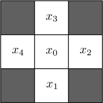
Figure 12: Illustration of the notation of the analysis on the ${L=3}$ square lattice. Note that the heights of the four corner sites (filled, gray) do not influence the volume retained by the lattice.

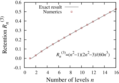
Figure 13: (Color online) Retention $R_{n}^{(3)}$ of an $n$-level system of size ${L=3}$ as function of $n$. The solid line is the exact result and the squares show the simulation data. The numerical results are averages over $10^{7}$ samples.

To confirm that the retention is monotonic in $n$ for small $L$ (see Fig. 4) and for further testing our simulation setup it is useful to compare the results with exactly solvable cases of the water retention model. As suggested in Ref. Knecht et al. (2012), we consider an $n$-level lattice of size ${L=3}$, see Fig. 12, and calculate $R_{n}^{(3)}$. The four corner sites of the lattice are irrelevant because, due to the geometry of the square lattice, their heights do not influence the retained volume. Let us call the height of the center site $x_{0}$. If any of the four heights $x_{1}$, $x_{2}$, $x_{3}$, or $x_{4}$ is lower than or equal to $x_{0}$, the retained volume of the configuration is zero. Otherwise, it is given by the difference between the lowest of the four relevant heights (where additional water would flow out to the border of the lattice) and the center height. Therefore, for a given configuration, the retained volume $V$ is given by

$$\begin{array}[]{lll}V(x_{0},x_{1},x_{2},x_{3},x_{4})&=&[\min\{x_{1},x_{2},x_{3},x_{4}\}-x_{0}]\\ &&\times\theta(x_{1}-x_{0})\theta(x_{2}-x_{0})\\ &&\times\theta(x_{3}-x_{0})\theta(x_{4}-x_{0}).\end{array}$$ (9)

The heights of the lattice sites are independently and uniformly distributed integers in $[0,n-1]$, therefore we have to calculate the average

$$R_{n}^{(3)}=\frac{1}{n^{5}}\sum_{x_{0}=0}^{n-1}\sum_{x_{1}=0}^{n-1}\sum_{x_{2}=0}^{n-1}\sum_{x_{3}=0}^{n-1}\sum_{x_{4}=0}^{n-1}V(x_{0},x_{1},x_{2},x_{3},x_{4}).$$ (10)

Inserting the expression for the volume given in Eq. (9) yields (see Ref. Knecht et al. (2012)):

$$R_{n}^{(3)}=\frac{(n^{2}-1)(2n^{2}-3)}{60n^{3}}.$$ (11)

Figure 13 shows the agreement between Eq. (11) and our simulation results. The result of Eq. (11) is also consistent with the decomposition of the retention capacity in Eq. (1): For two-level surfaces of size $3$ one has

$$R_{2}^{(3)}(p)=p(1-p)^{4}.$$ (12)

Inserting this into Eq. (1) recovers the result of Eq. (11).

References

- Knecht et al. (2012) C. L. Knecht, W. Trump, D. ben-Avraham, and R. M. Ziff, Phys. Rev. Lett. 108, 045703 (2012).
- Baek and Kim (2012) S. K. Baek and B. J. Kim, Phys. Rev. E 85, 032103 (2012).
- Kondev and Henley (1995) J. Kondev and C. L. Henley, Phys. Rev. Lett. 74, 4580 (1995).
- Kondev et al. (2000) J. Kondev, C. L. Henley, and D. G. Salinas, Phys. Rev. E 61, 104 (2000).
- Majumdar and Martin (2006) S. N. Majumdar and O. C. Martin, Phys. Rev. E 74, 061112 (2006).
- Schrenk et al. (2012) K. J. Schrenk, N. A. M. Araújo, J. S. Andrade Jr., and H. J. Herrmann, Sci. Rep. 2, 348 (2012).
- Schrenk et al. (2013) K. J. Schrenk, N. Posé, J. J. Kranz, L. V. M. van Kessenich, N. A. M. Araújo, and H. J. Herrmann, Phys. Rev. E 88, 052102 (2013).
- Barabási and Stanley (1995) A.-L. Barabási and H. E. Stanley, Fractal Concepts in Surface Growth (Cambridge University Press, New York, 1995).
- Araújo et al. (2002) A. D. Araújo, A. A. Moreira, H. A. Makse, H. E. Stanley, and J. S. Andrade Jr., Phys. Rev. E 66, 046304 (2002).
- Le Doussal and Wiese (2009) P. Le Doussal and K. J. Wiese, Phys. Rev. E 79, 051105 (2009).
- Xu et al. (1993) T. Xu, I. D. Moore, and J. C. Gallant, Geomorphology 8, 245 (1993).
- Czirók et al. (1993) A. Czirók, E. Somfai, and T. Vicsek, Phys. Rev. Lett. 71, 2154 (1993).
- Pastor-Satorras and Rothman (1998) R. Pastor-Satorras and D. H. Rothman, Phys. Rev. Lett. 80, 4349 (1998).
- Nikora et al. (1999) V. I. Nikora, C. P. Pearson, and U. Shankar, Landscape Ecol. 14, 17 (1999).
- Makse et al. (1998) H. A. Makse, J. S. Andrade Jr., M. Batty, S. Havlin, and H. E. Stanley, Phys. Rev. E 58, 7054 (1998).
- Carmi et al. (2008) S. Carmi, P. L. Krapivsky, and D. ben-Avraham, Phys. Rev. E 78, 066111 (2008).
- Sollich et al. (2008) P. Sollich, S. N. Majumdar, and A. J. Bray, J. Stat. Mech. , P11011 (2008).
- Fehr et al. (2011a) E. Fehr, D. Kadau, J. S. Andrade Jr., and H. J. Herrmann, Phys. Rev. Lett. 106, 048501 (2011a).
- Daryaei et al. (2012) E. Daryaei, N. A. M. Araújo, K. J. Schrenk, S. Rouhani, and H. J. Herrmann, Phys. Rev. Lett. 109, 218701 (2012).
- Andrade Jr. et al. (2011) J. S. Andrade Jr., S. D. S. Reis, E. A. Oliveira, E. Fehr, and H. J. Herrmann, Comput. Sci. Eng. 13, 74 (2011).
- Fehr et al. (2012) E. Fehr, K. J. Schrenk, N. A. M. Araújo, D. Kadau, P. Grassberger, J. S. Andrade Jr., and H. J. Herrmann, Phys. Rev. E 86, 011117 (2012).
- Fehr et al. (2011b) E. Fehr, D. Kadau, N. A. M. Araújo, J. S. Andrade Jr., and H. J. Herrmann, Phys. Rev. E 84, 036116 (2011b).
- Stauffer and Aharony (1994) D. Stauffer and A. Aharony, Introduction to Percolation Theory, 2nd ed. (Taylor and Francis, London, 1994).
- Wilkinson and Willemsen (1983) D. Wilkinson and J. F. Willemsen, J. Phys. A 16, 3365 (1983).
- Weinrib (1984) A. Weinrib, Phys. Rev. B 29, 387 (1984).
- Prakash et al. (1992) S. Prakash, S. Havlin, M. Schwartz, and H. E. Stanley, Phys. Rev. A 46, R1724 (1992).
- Schmittbuhl et al. (1993) J. Schmittbuhl, J.-P. Vilotte, and S. Roux, J. Phys. A 26, 6115 (1993).
- Mandre and Kalda (2011) I. Mandre and J. Kalda, Eur. Phys. J. B 83, 107 (2011).
- Olami and Zeitak (1996) Z. Olami and R. Zeitak, Phys. Rev. Lett. 76, 247 (1996).
- Saupe (1988) D. Saupe, in The Science of Fractal Images, edited by H.-O. Peitgen and D. Saupe (Springer, New York, 1988) p. 71.
- Makse et al. (1996) H. A. Makse, S. Havlin, M. Schwartz, and H. E. Stanley, Phys. Rev. E 53, 5445 (1996).
- Ballesteros and Parisi (1999) H. G. Ballesteros and G. Parisi, Phys. Rev. B 60, 12912 (1999).
- Ahrens and Hartmann (2011) B. Ahrens and A. K. Hartmann, Phys. Rev. B 84, 144202 (2011).
- Ziff (1998) R. M. Ziff, Comput. Phys. 12, 385 (1998).
- Matsumoto and Nishimura (1998) M. Matsumoto and T. Nishimura, ACM T. Model. Comput. S. 8, 3 (1998).
- Ziff (2011) R. M. Ziff, Phys. Procedia 15, 106 (2011).
- Riordan and Walters (2007) O. Riordan and M. Walters, Phys. Rev. E 76, 011110 (2007).
- Jacobsen (2014) J. L. Jacobsen, J. Phys. A 47, 135001 (2014).
- Schramm and Sheffield (2009) O. Schramm and S. Sheffield, Acta Math. 202, 21 (2009).
- Schwartz (2001) M. Schwartz, Phys. Rev. Lett. 86, 1283 (2001).
- Newman and Ziff (2000) M. E. J. Newman and R. M. Ziff, Phys. Rev. Lett. 85, 4104 (2000).
- Newman and Ziff (2001) M. E. J. Newman and R. M. Ziff, Phys. Rev. E 64, 016706 (2001).
- Hu et al. (2012) H. Hu, H. W. J. Blöte, and Y. Deng, J. Phys. A 45, 494006 (2012).
- Weinrib and Halperin (1983) A. Weinrib and B. I. Halperin, Phys. Rev. B 27, 413 (1983).
- Sandler et al. (2004) N. Sandler, H. R. Maei, and J. Kondev, Phys. Rev. B 70, 045309 (2004).
- Saberi (2013) A. A. Saberi, Phys. Rev. Lett. 110, 178501 (2013).