A comparative simulation study of data-driven methods for estimating density level sets

Abstract

Density level sets are mainly estimated using one of three methodologies: plug-in, excess mass, or a hybrid approach. The plug-in methods are based on replacing the unknown density by some nonparametric estimator, usually the kernel. Thus, the bandwidth selection is a fundamental problem from a practical point of view. Recently, specific selectors for level sets have been proposed. However, if some a priori information about the geometry of the level set is available, then excess mass algorithms can be useful. In this case, a density estimator is not necessary, and the problem of bandwidth selection can be avoided. The third methodology is a hybrid of the others. As in the excess mass method, it assumes a mild geometric restriction on the level set and, like the plug-in approach, requires a pilot nonparametric estimator of the density. One interesting open question concerns the practical performance of these methods. In this work, existing methods are reviewed, and two new hybrid algorithms are proposed. Their practical behaviour is compared through extensive simulations.

1 Introduction

Level set estimation theory deals with the problem of reconstructing an unknown set $L(\tau)=\{f\geq f_{\tau}\}$ from a random sample of points $\mathcal{X}_{n}=\{X_{1},...,X_{n}\}$ of a random variable $X$, where $f$ is the density of $X$, $\tau\in(0,1)$ is a given probability, and $f_{\tau}>0$ denotes the largest threshold such that the level set $L(\tau)$ has a probability greater than or equal to $1-\tau$ with respect to the distribution induced by $f$. Figure 1 shows the level sets for three different values of the parameter $\tau$. For values of $\tau$ close to one, the level set represents the domain concentrated around the greatest mode. However, if $\tau$ is close to zero, then it represents the effective support of the density $f$.

Figure 1: Level sets for a $1-$dimensional density with $\tau=0.1$ (left), $\tau=0.5$ (centre), and $\tau=0.9$ (right).

Level set estimation plays a crucial role in various scientific fields, and has received considerable interest in the literature. Since Hartigan (1975) introduced the notion of population clusters as the connected components of density level sets, many interesting applications have appeared. The concept of clustering is related to the notion of the mode and, in fact, some clustering algorithms are based on the estimation of modes (see Cuevas, Febrero and Fraiman, 2000). An interesting application of this clustering approach to astronomical sky surveys was proposed by Jang (2006), and Klemelä (2004, 2006) used a similar point of view to develop methods for visualizing multivariate density estimates. Goldenshluger and Zeevi (2004) used level set estimation in the context of the Hough transform, which is a well-known computer vision algorithm. Some problems in flow cytometry involve the statistical problem of reconstructing a level set for the difference between two probability densities (see Roederer and Hardy, 2001). In addition, interesting applications include the detection of mine fields based on aerial observations, the analysis of seismic data, as well as certain issues in image segmentation (see Huo and Lu, 2004). The detection of outliers is another important application of level set estimation (see Gardner et al. (2006) or Markou and Singh (2003) for a review). An outlier can be thought of as an observation that is in the set $\{f<f_{\tau}\}$. In other words, the outlier does not belong to the effective support determined by the level set $L(\tau)$. This approach follows that of Devroye and Wise (1980) to determine whether a manufacturing process is out of control. For quality control schemes, see also Baíllo, Cuevas and Justel (2000) or Baíllo and Cuevas (2006).

The broad scope of level set estimation clearly motivates the need for an in-depth study of the practical performance of existing methods. In general, the problem has been approached using three different nonparametric methodologies: plug-in methods, excess mass methods, and hybrid methods (for a Bayesian alternative, see Gayraud and Rousseau, 2005). This paper focuses on analyzing the behaviour of existing data-driven methods for reconstructing density level sets. The three types of data-driven algorithms for the estimation of level sets will be presented and compared through a detailed simulation study. We focus on the one-dimensional setting so as to include some methods that do not have multidimensional counterparts, such as the plug-in algorithm proposed by Samworth and Wand (2010) or the excess mass method developed by Müller and Sawitzki (1991).

This paper is organized as follows. Plug-in methods are presented and compared in Section 2. Sections 3 and 4 discuss the behaviour of excess mass and hybrid methods, respectively. In addition, two new hybrid algorithms are proposed in Section 4. The most competitive methods in each group are then compared in Section 5. Finally, we present some general conclusions in Section 6.

2 Comparative study of plug-in methods

The simplest option for estimating level sets is the so-called plug-in methodology. This is based on replacing the unknown density $f$ by a suitable nonparametric estimator $f_{n}$, usually that of the kernel. Given $\mathcal{X}_{n}$, the kernel density estimator at a point $x$ is defined as

$$f_{n}(x)=\frac{1}{nh}\sum_{i=1}^{n}K\left(\frac{X_{i}-x}{h}\right),\vspace{.1 cm}$$

where $K$ denotes a kernel function (in what follows, the Gaussian kernel) and $h>0$ denotes the bandwidth parameter. Thus, this group of methods proposes $\hat{L}(\tau)=\{f_{n}\geq\hat{f}_{\tau}\}$ as an estimator of $L(\tau)$, where $\hat{f}_{\tau}$ estimates $f_{\tau}$ as follows:

1. Through numerical integration methods by solving

   $$\int_{\{f_{n}\geq t\}}f_{n}(x)dx=1-\tau\vspace{.1cm}$$

   for $t$. This algorithm is consistent with the plug-in philosophy, as $\hat{f}_{\tau}$ is the corresponding threshold if $f$ is replaced by $f_{n}$. However, this may be inefficient from a computational point of view. For consistency results, see Cadre (2006).

2. Hyndman (1996) proposed a method for estimating $f_{\tau}$ by calculating the $\tau-$quantile of the empirical distribution of $f_{n}(X_{1}),...,f_{n}(X_{n})$. The computational cost of this approach is lower than that of the previous method. For consistency results, see Cadre, Pelletier and Pudlo (2013).

The plug-in methodology is the most common approach, and has received considerable attention in the literature, e.g., Tsybakov (1997), Baíllo (2003), Mason and Polonik (2009), Rigollet and Vert (2009), or Mammen and Polonik (2013). However, its performance is heavily dependent on the choice of the bandwidth parameter $h$ for estimating $f$, and there are many methods of selecting $h$ in the density estimation. Next, we review existing specific bandwidth selectors for density level set estimation.

Baíllo and Cuevas (2006) used quality control ideas to estimate level sets. In this context, $L(\tau)$ can be seen as a population tolerance region. Let us assume that a machine working in normal operation produces a sequence of independent observations $\mathcal{X}_{n}$ drawn from the density $f$. For example, $X_{i}$ could be a value for a certain quality characteristic of a manufactured product. If the process starts to run out of control, the distribution of the samples will change. The aim is to detect a real change in this distribution as soon as possible, subject to the bound $\tau\in(0,1)$ on the rate of false alarms. The key idea is that, if there is no change in the distribution for a new observation, then it is most likely to be within the tolerance limits of the region $L(\tau)$. In practice, we may determine that the $n+1$-th observation is a change-point in the distribution of the process, that is, a new observation $X_{n+1}$ does not follow the distribution of $\mathcal{X}_{n}$ if $X_{n+1}$ does not belong to the plug-in estimator of $L(\tau)$. Hence, choosing a good smoothing parameter to reconstruct a level set in the context of quality control is an interesting problem. Cuevas and Baíllo (2006) proposed a bandwidth selector by minimizing a cross-validation estimate of $|\mathbb{P}_{f_{n}}(h)-\tau|\mbox{ where }\mathbb{P}_{f_{n}}(h)=\int_{\{f_{n}<\hat{f}_{\tau}\}}f$ denotes the probability of a false alarm. Specifically, $\mathbb{P}_{f_{n}}(h)$ is approximated by

$$\mathbb{P}_{CV}(h)=\frac{1}{n}\sum_{i=1}^{n}\mathbb{I}_{\{f_{n,-i}(X_{i})<\hat{f}_{\tau,-i}\}},\vspace{.13 cm}$$

where $f_{n,-i}$ is the kernel estimator with bandwidth $h$, constructed from $X_{1},...,X_{i-1},X_{i+1},...,X_{n}$, and $\hat{f}_{\tau,-i}$ satisfies

$$\int_{\{f_{n,-i}\geq\hat{f}_{\tau,-i}\}}f_{n,-i}=1-\tau.\vspace{.13 cm}$$

Samworth and Wand (2010) proposed a new automatic rule to select the smoothing parameter in the one-dimensional case. Their proposal is based on a uniform-in-bandwidth asymptotic approximation of a specific set estimation risk function, $\mathbb{E}\{d_{\mu_{f}}(L(\tau),\hat{L}(\tau))\}$, where

$$d_{\mu_{f}}(L(\tau),\hat{L}(\tau))=\int_{L(\tau)\triangle\hat{L}(\tau)}f(t)\mbox{ }dt\vspace{.1 cm}$$

and $\triangle$ denotes the symmetric difference given by $L(\tau)\triangle\hat{L}(\tau)=(L(\tau)\setminus\hat{L}(\tau))\cup(\hat{L}(\tau)\setminus L(\tau))$. This asymptotic approximation of the risk function was used to develop a plug-in bandwidth selection strategy by minimizing an estimator of the asymptotic risk. It was proved that, under some smoothness assumptions on $f$, the solution to this minimization problem is, with probability one, unique for large $n$. The asymptotic risk depends on the threshold $f_{\tau}$, the density function, and its first and second derivatives ($f^{{}^{\prime}}$ and $f^{{}^{\prime\prime}}$, respectively) evaluated at the unknown extremes $x_{1},...,x_{2r}$ of the intervals that form the theoretical level set. These three functions are estimated using kernel estimators with different pilot bandwidths $\hat{h}_{0}$, $\hat{h}_{1}$, and $\hat{h}_{2}$ for $f$, $f^{{}^{\prime}}$, and $f^{{}^{\prime\prime}}$, respectively. The kernel estimators can then be denoted by $f_{n,\hat{h}_{0}}$, $f_{n,\hat{h}_{1}}^{{}^{\prime}}$, and $f_{n,\hat{h}_{2}}^{{}^{\prime\prime}}$. The threshold $f_{\tau}$ is estimated by numerical integration from $f_{n,\hat{h}_{0}}$, whereas the points $x_{1},...,x_{2r}$ are estimated by solving the equation $f_{n,\hat{h}_{0}}(x)=\hat{f}_{\tau}$. However, it should be noted that this algorithm can provide level set estimators that are equal to the empty set, mainly for large values of $\tau$. The reason for this is simple—the estimation of the pilot bandwidth $\hat{h}_{0}$, which is used to estimate the threshold $f_{\tau}$, can be considerably greater than the final smoothing parameter $\hat{h}_{SW}$ obtained by Samworth and Wand’s algorithm. The density estimator calculated from $\hat{h}_{SW}$ does not then intersect $\hat{f}_{\tau}$. To solve this problem, the threshold must be recalculated from $\hat{h}_{SW}$ after obtaining it. The modified version of this method will be considered in the rest of this paper.

Singh, Scott and Nowak (2009) presented a plug-in procedure for reconstructing density level sets based on a histogram. This method considers a collection of cells $A$ as a regular partition of $[0,1]^{d}$ ($d\geq 1$) into hypercubes $\mathcal{A}_{j}$ of dyadic sidelength $2^{-j}$, where $j$ is a nonnegative integer. The estimator of the level set $C(\lambda)=\{f\geq\lambda\}$ for a given value of $\lambda>0$ at a resolution level of $j$ is defined as

$$\hat{C}(\lambda)=\bigcup_{\{A\in\mathcal{A}_{j}:f_{n,H}(A)\geq\lambda\}}A\mbox{ with }f_{n,H}(A)=\frac{\mathbb{P}_{n}(A)}{\mu(A)},\vspace{.12 cm}$$

where $\mathbb{P}_{n}$ denotes the empirical probability induced by $\mathcal{X}_{n}$ and $\mu$ is the Lebesgue measure. $L(\tau)$ can be estimated by $\hat{C}(\hat{f}_{\tau})$ where, to avoid the problem of bandwidth selection, $\hat{f}_{\tau}$ is computed using the empirical procedure proposed by Walther (1997). That is,

$$\hat{f}_{\tau}=\max\{\lambda>0:\mathbb{P}_{n}(\hat{C}(\lambda))\geq 1-\tau\}.\vspace{.12 cm}$$

The algorithm suggested in Singh, Scott and Nowak (2009) depends on the resolution level $j$. This parameter is selected using a data-driven procedure (see Section 3.2 in Singh, Scott and Nowak, 2009). It was proved that near-minimax optimal rates of convergence for a specific class of level sets are achieved for the resulting density level set estimator.

Of course, it is also possible to consider classical methods such as cross-validation (see Bowman, 1984) or plug-in algorithms (see Sheather and Jones, 1991) to select the bandwidth parameter, although these are not specific to the estimation of level sets.

2.1 Simulations results for plug-in methods

In this section, we compare the methods of Baíllo and Cuevas (BC), Samworth and Wand (SW), Sheather and Jones (SJ), and cross-validation (CV). BC and SW are specific bandwidth selectors for estimating level sets. The latter two algorithms are general selectors for the estimation of density functions. The behaviour of these general methods has been studied in the context of density level set estimation, e.g., in Cao, Cuevas and González-Manteiga (1994). The results of Singh, Scott and Nowak’s algorithm are not included in this comparison because, for the sample size considered in the study, its behaviour was not satisfactory.

Figure 2: Density models for the simulation study.

We generated $1000$ samples of size $n=1600$ from 18 density models (see Figure 2). Models 1–15 are the densities proposed by Marron and Wand (1992). Models 16–18 correspond to the marronite, caliper, and matterhorn densities proposed in Berlinet and Devroye (1994). These models were added because they present some special properties. Specifically, they have two asymmetric and separated modes, two jumps, and a non-finite peak, respectively.

In addition, three values of the parameter $\tau$ have been considered: $\tau=0.2$, $\tau=0.5$, and $\tau=0.8$. The threshold $f_{\tau}$ was estimated using the two procedures described previously. Although the comparison is not shown, the two algorithms for estimating $f_{\tau}$ provided similar results. Therefore, in the following, only the results for Hyndman’s method will be considered. The bandwidth given by Sheather and Jones has been used as the pilot selector to calculate $f_{n}$ for the estimation of $f_{\tau}$.

For each fixed random sample and each method, we calculated the estimator $\hat{L}(\tau)$ of $L(\tau)$ and the error in the estimation $d_{\mu_{f}}(L(\tau),\hat{L}(\tau))$. Thus, $1000$ errors were obtained for each algorithm, model, and value of $\tau$. To facilitate the presentation of the results, the following figures are divided into rectangles of different colours according to the method (vertical axis) and density model (horizontal axis), where light colours correspond to small errors, and vice versa. This representation allows us to detect the most competitive algorithm for each fixed value of $\tau$ and model. Given a density, the empirical means of the $1000$ errors have been ordered by testing whether the mean errors of the compared methods are equal. If the null hypothesis of equality between two methods is rejected, then each algorithm is painted a different colour (darker or lighter according to the mean error). Otherwise, both algorithms are represented using the same colour. This approach will be used in the rest of the paper.

Figures 3, 4, and 5 compare the plug-in methods for $\tau=0.2$, $\tau=0.5$, and $\tau=0.8$, respectively. Clearly, the general bandwidth selectors exhibit the best global behaviour for $\tau=0.2$ and $\tau=0.5$. When $\tau=0.8$, the classical selectors again produce the best results for models 4, 6, 8, 9, 10, 11, 12, 13, 14, 15, 16, and 17. Some of these models are quite sophisticated densities. In this case, specific selectors are only competitive for quite simple models, such as 1, 2, 3, 5, 7, and 18 in Figure 5. All of these densities are unimodal or simple bimodal models.

In particular, if $\tau=0.2$ or $\tau=0.5$, SW behaves better than BC (see densities 10, 11, 12, 14, and 15 in Figures 3 and 4). However, BC provides better results than SW for $\tau=0.8$ (see models 3, 5, 6, 7, 8, 9, 10, 11, 13, 15, 16, and 17 in Figure 5).

Less competitive More competitive

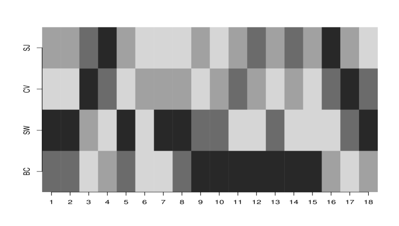
Figure 3: Comparison of plug-in methods (vertical axis) with the 18 model densities (horizontal axis), $\tau=0.2$ and $n=1600$.

Less competitive More competitive

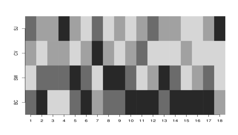
Figure 4: Comparison of plug-in methods (vertical axis) with the 18 model densities (horizontal axis), $\tau=0.5$ and $n=1600$.

Less competitive More competitive

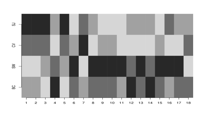
Figure 5: Comparison of plug-in methods (vertical axis) with the 18 model densities (horizontal axis), $\tau=0.8$ and $n=1600$.

In conclusion, specific methods to estimate level sets, such as those of Samworth and Wand, Baíllo and Cuevas, or Singh, Clayton and Nowak, do not improve the results of the classic bandwidth selection rules, at least for the sample sizes considered here. In addition, the CV and SJ methods often provide similar results, and present the best global behaviour.

3 Comparative study of excess mass methods

Another possibility is to assume that the set of interest satisfies some geometric condition, such as convexity. In this case, the excess mass approach, first proposed by Hartigan (1987) and Müller and Sawitzki (1987), provides an alternative for the reconstruction of density level sets. Some previous contributions can be seen in Chernoff (1964) or Eddy and Hartigan (1977). This group of algorithms utilizes the fact that the density level set $C(\lambda)=\{f\geq\lambda\}$, for a given value of $\lambda>0$, maximizes the functional

$$H_{\lambda}(B)=\mathbb{P}(B)-\lambda\mu(B),$$

where $\mathbb{P}$ is the probability measure induced by $f$ and $\mu$ is the Lebesgue measure. If $\mathcal{B}$ is a given class of sets, then a natural estimator $\hat{C}(\lambda)$ of $C(\lambda)$, under the shape restriction $C(\lambda)\in\mathcal{B}$, would be the maximizer of the empirical excess mass

$$H_{\lambda,n}(B)=\mathbb{P}_{n}(B)-\lambda\mu(B)$$

on $\mathcal{B}$, where $\mathbb{P}_{n}$ denotes the empirical probability induced by the sample $\mathcal{X}_{n}$. This method incorporates geometric information in a natural way. If no shape restriction is assumed, the maximizer of $H_{\lambda,n}$ would be $\mathcal{X}_{n}$. Hartigan (1987) and Grübel (1988) considered the case where $\mathcal{B}$ is the class of convex sets in the two- and one-dimensional cases, respectively. Asymptotic estimator results for more general classes $\mathcal{B}$ were given by Polonik (1995).

According to the previous comments, the goal of this work is to reconstruct density level sets with a fixed probability content. To avoid the bandwidth selection problem, and again following the empirical procedure proposed by Walther (1997), $\hat{L}(\tau)=\hat{C}(\hat{f}_{\tau})$, where

$$\hat{f}_{\tau}=\max\{\lambda>0:\mathbb{P}_{n}(\hat{C}(\lambda))\geq 1-\tau\}.$$

This methodology has been widely studied in the literature. Müller and Sawitzki (1991) proposed an efficient algorithm for estimating one-dimensional sets by assuming that the theoretical level set can be written as a finite union of $M$ closed intervals. This algorithm assumes that $M$ is known a priori.

3.1 Simulation results for excess mass methods

Müller and Sawitzki’s method depends on a parameter $M$, which, if unknown, presents the main disadvantage of this algorithm. Five values for the number of clusters have been considered, $M=1,\mbox{ }2,\mbox{ }3,\mbox{ }4,$ and $5$. The Müller and Sawitzki’s method with $M$ modes will be denoted by MS_M.

Figure 6 shows the simulation results for the five values of $M$ with $\tau=0.5$ and $n=1600$. These can be used to analyze the influence of $M$ in the method of Müller and Sawitzki. The real number of modes for each density when $\tau=0.5$ has been included at the top of the vertical axis. It is clear that Müller and Sawitzki’s algorithm is very sensitive to the parameter $M$. For $\tau=0.5$, densities 1–5 are unimodal, and MS₁ provides the best results. Densities 6–8 have two modes and, in this case, the best algorithm is MS₂. However, for the two modes of model 9, MS₃ provides the best results. Model 10 has five modes for $\tau=0.5$, and here MS₅ produces the best estimations. However, the optimum value of $M$ for Müller and Sawitzki’s method is not equal to the real value of $M$ for models 11, 12, and 13, because some of their modes are not significant. In addition, if $M$ is misspecified, larger values of $M$ tend to be better than smaller ones (see models 6–9).

Less competitive More competitive

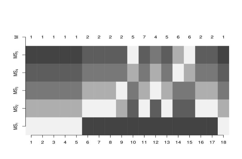
Figure 6: Comparison of Müller and Sawitzki’s method for different values of $M$ (vertical axis) with the 18 model densities (horizontal axis), $\tau=0.5$ and $n=1600$. The real number of modes for each density has been included at the top of the vertical axis.

4 Comparative study of hybrid methods

As the name suggests, hybrid methods assume a priori geometric restrictions on $L(\tau)$, and they also use a pilot nonparametric density estimator to define the set $\mathcal{X}_{n}^{+}=\{X_{i}\in\mathcal{X}_{n}:f_{n}(X_{i})\geq\hat{f}_{\tau}\}$. In this paper, two new hybrid methods to estimate convex and $r$-convex ($r>0$) sets are proposed. This latter shape restriction generalizes the convexity assumption. A closed set $A$ is said to be $r$-convex for some $r>0$ if $A=C_{r}(A)$, where

$$C_{r}(A)=\bigcap_{\{B_{r}(x):B_{r}(x)\cap A=\emptyset\}}\left(B_{r}(x)\right)^{c}$$

denotes the $r$-convex hull of $A$, $B_{r}(x)$ is the open ball with centre $x$ and radius $r$, and $\left(B_{r}(x)\right)^{c}$ is its complement. Our two new proposals are based on the convex hull and $r$-convex hull methods for estimating the support (see Korostelëv and Tsybakov (1993) and Rodríguez-Casal (2007), respectively). Under the convexity restriction, it is shown that we can estimate the level set as the convex hull of $\mathcal{X}_{n}^{+}$ and, under the $r$-convexity assumption, as the $r$-convex hull of $\mathcal{X}_{n}^{+}$. Another classic hybrid technique is the granulometric smoothing method (see Walther, 1997). This assumes that the level set $L(\tau)$ and its complement are both $r$-convex. This method adapts the support estimator proposed by Devroye and Wise (1980) to the context of level set estimation. In this case, the estimator is defined as the union of balls of radius $r$ around those points in $\mathcal{X}_{n}^{+}$ that are a distance of at least $r$ from each point in $\mathcal{X}_{n}\setminus\mathcal{X}_{n}^{+}$.

4.1 Simulation results for hybrid methods

Granulometric smoothing and the $r$-convex hull method depend on the unknown parameter $r$. This is the main disadvantage of these algorithms. In this work, five fixed values for the radius have been considered: $r_{1}=0.01$, $r_{2}=0.05$, $r_{3}=0.1,$ $r_{4}=0.2$, and $r_{5}=0.3$. Although not discussed here, the influence of the parameter $r$ on the $r$-convex hull method and granulometric smoothing has been studied, and in general, the $r$-convex hull method is less sensitive to the selection of $r$.

We denote the convex hull method as CH, the $r$-convex hull method as CH_r, and granulometric smoothing with radius $r$ as W_r. The latter two methods have been compared by fixing $r=r_{3}$. For the first two, the threshold was calculated using Hyndman’s method by taking Sheather and Jones’ bandwidth as the pilot selector to calculate $f_{n}$. For W_r, the threshold was estimated empirically according to Walther’s proposal.

Figures 7, 8, and 9 show the results obtained for $\tau=0.2$, $\tau=0.5$, and $\tau=0.8$, respectively. Each method is represented on the vertical axis, and each density model on the horizontal axis.

Some density models present convex level sets for $\tau=0.2$, although they are not unimodal (for example, densities 6, 8, or 11). In these cases, when the convexity assumption is true, CH can be very competitive. However, models 1–4 have convex level sets for any value of $\tau$, and the $r_{3}$-convex hull method is then the most competitive. In addition, sometimes the convexity hypothesis can be very restrictive (models 7 or 10, for example), and in such cases the $r_{3}$-convex hull method or granulometric smoothing provide better results.

Less competitive More competitive

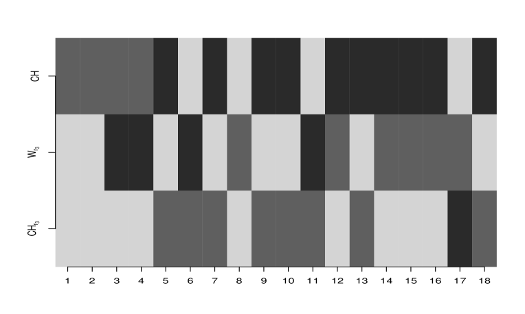
Figure 7: Comparison of hybrid methods (vertical axis) with the 18 model densities (horizontal axis), $\tau=0.2$ and $n=1600$.

Less competitive More competitive

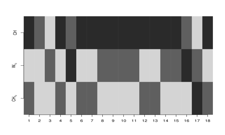
Figure 8: Comparison of hybrid methods (vertical axis) with the 18 model densities (horizontal axis), $\tau=0.5$ and $n=1600$.

Less competitive More competitive

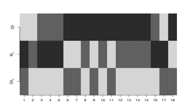
Figure 9: Comparison of hybrid methods (vertical axis) with the 18 model densities (horizontal axis), $\tau=0.8$ and $n=1600$.

When $\tau=0.5$, convexity is a very restrictive shape condition for most of the models (see densities 6–15). Granulometric smoothing and the $r_{3}$-convex hull method have better behaviour than CH in this case. The $r_{3}$-convex hull algorithm is quite competitive for multimodal models, such as for densities 8, 9, 10, 11, 14, and 15.

Although Walther’s method and the $r_{3}$-convex hull algorithm provide similar results for $\tau=0.2$ and $\tau=0.5$, the new proposal is clearly better for high values of $\tau$—see unimodal models 2, 3, 4, 5, and 8 or more complex densities 10, 12, 13, 14, 15, and 16 in Figure 9. Granulometric smoothing is only the most competitive method for densities 6, 7, 9, 11, and 18. The first three have quite simple level sets, with only two connected components, whereas model 11 presents seven modes, five of which are not significant.

Note that the $r_{3}$-convex hull method does not provide the worst result for any of the models considered. This is quite promising, because the parameter $r$ is not estimated from the data, and it was expected that this would change from model to model.

5 Final comparison

Finally, we compared the most competitive methods in each group: cross-validation, Müller and Sawitzki’s method, granulometric smoothing, and the $r$-convex hull method. It is necessary to specify values for $M$ and $r$ for Müller and Sawitzki’s method, granulometric smoothing, and the $r$-convex hull method. We therefore considered $M=1$, $M=2$, and $r=r_{3}$.

Figures 10, 11, and 12 show the results for $\tau=0.2$, $\tau=0.5$, and $\tau=0.8$, respectively. When $\tau=0.2$, Müller and Sawitzki’s method is more competitive with $M=1$ than with $M=2$ for unimodal densities of 1–5, as shown in Figure 10. The same conclusion can be extracted for models 6, 8, 11, and 18, because, for this value of $\tau$, their level sets have only one interval. Müller and Sawitzki’s method with $M=2$ does not exhibit very good results, because most of the models are not bimodal. In spite of this, it is the most competitive algorithm for models 10, 12, and 16. In this case, cross-validation provides quite good results, except for densities 3, 4, 6, 7, 9, 11, and 17, where one of the two hybrid methods presents the best behaviour. However, these two algorithms have a very important disadvantage in that they depend on an unknown parameter.

When $\tau=0.5$, the cross-validation selector provides quite competitive results (see models 1, 2, 4, 5, 6, 10, 12, 14, 16, 17, and 18 in Figure 11). Granulometric smoothing and the $r_{3}$-convex hull method produce the best results for densities 6, 7, and 8 and 3, 8, 9, 11, 15, and 16, respectively. In this case, Müller and Sawitzki’s method is not particularly competitive, especially when $M=1$ for models 6–17. All of these densities have level sets with more than one interval.

Cross-validation exhibits the most competitive behaviour for unimodal densities when $\tau=0.8$ (see models 1, 2, 4, 5, 8, and density 16 in Figure 12). Granulometric smoothing presents its worst performance for densities 3, 4, 5, and 16. However, although the $r_{3}$-convex hull method is not the most competitive for many of the models, it presents very regular behaviour. Müller and Sawitzki’s method with $M=1$ does not provide very good results, e.g., densities 6, 7, 9, 10, 11, 12, 14, and 15. None of these models are unimodal. If we consider $M=2$, this method is the most competitive for densities 12, 13, and 17.

Less competitive More competitive

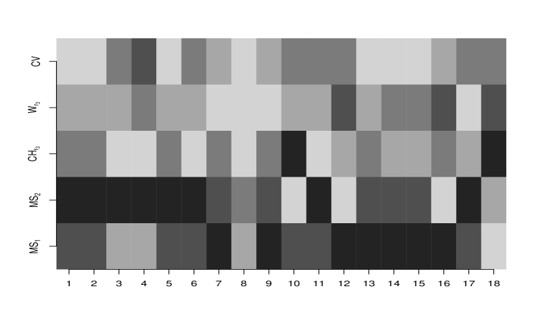
Figure 10: Comparison of CV, W${}_{r_{3}}$, CH${}_{r_{3}}$, MS₂, and MS₁ (vertical axis) with the 18 model densities (horizontal axis), $\tau=0.2$ and $n=1600$.

Less competitive More competitive

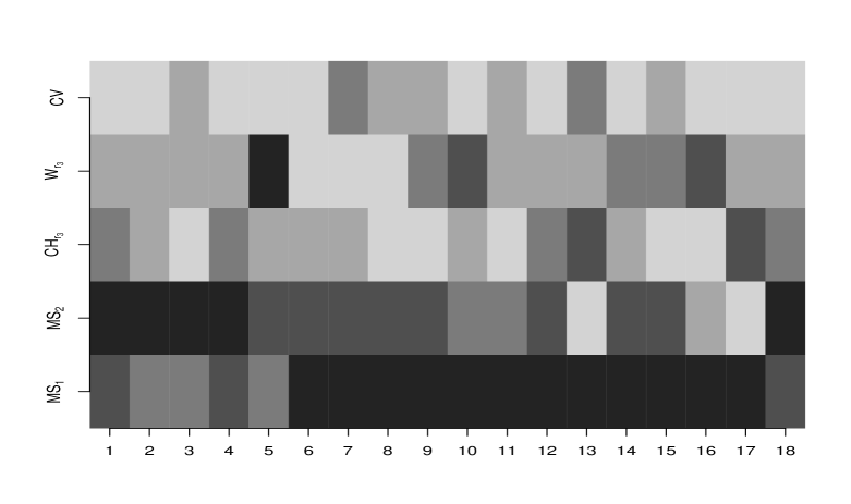
Figure 11: Comparison of CV, W${}_{r_{3}}$, CH${}_{r_{3}}$, MS₂, and MS₁ (vertical axis) with the 18 model densities (horizontal axis), $\tau=0.5$ and $n=1600$.

Less competitive More competitive

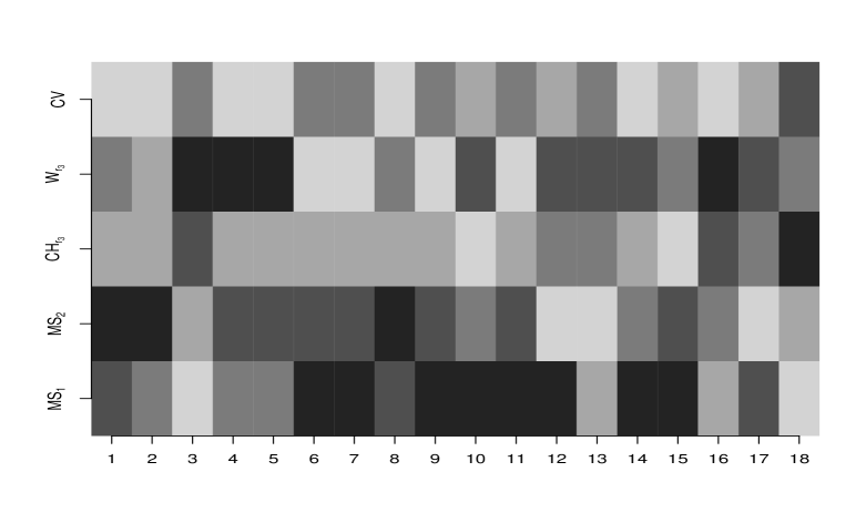
Figure 12: Comparison of CV, W${}_{r_{3}}$, CH${}_{r_{3}}$, MS₂, and MS₁ (vertical axis) with the 18 model densities (horizontal axis), $\tau=0.8$ and $n=1600$.

6 Conclusions

As has been stated previously, if no assumption is made on the shape of the density level set to be estimated, then plug-in methods provide good results. In general, cross-validation or even Sheather and Jones’ method are good alternatives for reconstructing the level set. Previous results suggest that specific bandwidth selectors for density level sets present worse general behaviour for the sample size considered.

In contrast, excess mass and hybrid methods are useful for incorporating the shape restrictions of the density level set into the estimators. In particular, Müller and Sawitzki’s algorithm assumes that some information about the number of clusters $M$ is given a priori. We therefore fixed two values, $M=1$ and $M=2$. Although most model densities satisfy one of these two conditions, this algorithm did not provide very competitive results. However, one of the main advantages of the excess mass methodology is that it does not need to smooth the data to reconstruct a density level set with a fixed probability content.

If, however, some geometric properties of the level set are known, then hybrid methods present a competitive alternative. For instance, if $\tau$ is small, the convex hull method was shown to provide good results. Most of these densities have convex level sets for sufficiently small values of $\tau$. Under more flexible shape restrictions, the $r$-convex hull method and granulometric smoothing could be used. However, their main disadvantage is the dependence on $r$, an unknown parameter. These approaches are very promising, because they remain quite competitive even when the value of $r$ is fixed. Selecting $r$ automatically from the sample points would significantly improve their practical performance.

Acknowledgments. This work has been supported by Project MTM2008-03010 of the Spanish Ministry of Science and Innovation and the IAP network StUDyS (Developing crucial Statistical methods for Understanding major complex Dynamic Systems in natural, biomedical and social sciences) of the Belgian Science Policy.

References

- [1] A. Baíllo. Total error in a plug-in estimator of level sets. Statistics & Probability Letters, 65(4):411–417, 2003.
- [2] A. Baíllo and A. Cuevas. Parametric versus nonparametric tolerance regions in detection problems. Computational Statistics, 21(3-4):523–536, 2006.
- [3] A. Baíllo, A. Cuevas, and A. Justel. Set estimation and nonparametric detection. The Canadian Journal of Statistics, 28(4):765–782, 2000.
- [4] A. Berlinet and L. Devroye. A comparison of kernel density estimates. Publications de l’Institut de Statistique de l’Université de Paris, 38(3):3–59, 1994.
- [5] A. W. Bowman. An alternative method of cross-validation for the smoothing of density estimates. Biometrika, 71(2):353–360, 1984.
- [6] B. Cadre. Kernel estimation of density level sets. Journal of Multivariate Analysis, 97(4):999–1023, 2006.
- [7] B. Cadre, B. Pelletier, and P. Pudlo. Estimation of density level sets with a given probability content. Journal of Nonparametric Statistics, 25(1):261–272, 2013.
- [8] R. Cao, A. Cuevas, and W. González-Manteiga. A comparative study of several smoothing methods in density estimation. Computational Statistics & Data Analysis, 17(2):153–176, 1994.
- [9] H. Chernoff. Estimation of the mode. Annals of the Institute of Statistical Mathematics, 16(1):31–41, 1964.
- [10] A. Cuevas, M. Febrero, and R. Fraiman. Estimating the number of clusters. The Canadian Journal of Statistics, 28(2):367–382, 2000.
- [11] L. Devroye and G. L. Wise. Detection of abnormal behavior via nonparametric estimation of the support. SIAM Journal on Applied Mathematics, 38(3):480–488, 1980.
- [12] W. F. Eddy and J. A. Hartigan. Uniform convergence of the empirical distribution function over convex sets. The Annals of Statistics, 5(2):370–374, 1977.
- [13] A. B. Gardner, A. M. Krieger, G. Vachtsevanos, and B. Litt. One-class novelty detection for seizure analysis from intracranial EEG. The Journal of Machine Learning Research, 7:1025–1044, 2006.
- [14] G. Gayraud and J. Rousseau. Rates of convergence for a bayesian level set estimation. Scandinavian Journal of Statistics, 32(4):639–660, 2005.
- [15] A. Goldenshluger and A. Zeevi. The hough transform estimator. The Annals of Statistics, 32(5):1908–1932, 2004.
- [16] R. Grübel. The length of the shorth. The Annals of Statistics, 16(2):619–628, 1988.
- [17] J.A. Hartigan. Clustering Algorithms. Wiley, 1975.
- [18] J.A. Hartigan. Estimation of a convex density contour in two dimensions. Journal of the American Statistical Association, 82(397):267–270, 1987.
- [19] X. Huo and J. C. Lu. A network flow approach in finding maximum likelihood estimate of high concentration regions. Computational Statistics & Data Analysis, 46(1):33–56, 2004.
- [20] R. J. Hyndman. Computing and graphing highest density regions. The American Statistician, 50(2):120–126, 1996.
- [21] W. Jang. Nonparametric density estimation and clustering in astronomical sky surveys. Computational Statistics & Data Analysis, 50(3):760–774, 2006.
- [22] J. Klemelä. Visualization of multivariate density estimates with level set trees. Journal of Computational & Graphical Statistics, 13(3):599–620, 2004.
- [23] J. Klemelä. Visualization of multivariate density estimates with shape trees. Journal of Computational and Graphical Statistics, 15(2), 2006.
- [24] A. P. Korostelev and A. B. Tsybakov. Minimax Theory of Image Reconstruction. Springer, 1993.
- [25] E. Mammen and W. Polonik. Confidence regions for level sets. Journal of Multivariate Analysis, 122(0):202–214, 2013.
- [26] M. Markou and S. Singh. Novelty detection: a review part 1: statistical approaches. Signal Processing, 83(12):2481–2497, 2003.
- [27] J. S. Marron and M. P. Wand. Exact mean integrated squared error. The Annals of Statistics, 20(2):712–736, 1992.
- [28] D. M. Mason and W. Polonik. Asymptotic normality of plug-in level set estimates. The Annals of Applied Probability, 19(3):1108–1142, 2009.
- [29] D. W. Müller and G. Sawitzki. Using Excess Mass Estimates to Investigate the Modality of Distribution. Sonderforschungsbereich, Heidelberg University, 1987.
- [30] D.W. Müller and G. Sawitzki. Excess mass estimates and tests of multimodality. Journal of the American Statistical Association, 86(415), 1991.
- [31] W. Polonik. Measuring mass concentrations and estimating density contour clusters - an excess mass approach. The Annals of Statistics, 23(3):855–881, 1995.
- [32] P. Rigollet and R. Vert. Optimal rates for plug-in estimators of density level sets. Official Journal of the Bernoulli Society for Mathematical Statistics and Probability, 15(4):1154–1178, 2009.
- [33] A. Rodríguez-Casal. Set estimation under convexity type assumptions. Annales de l’Institut Henri Poincaré - Probabilités & Statistiques, 43(6):763–774, 2007.
- [34] M. Roederer and R. R. Hardy. Frequency difference gating: a multivariate method for identifying subsets that differ between samples. Cytometry, 45(1):56–64, 2001.
- [35] R.J. Samworth and M.P. Wand. Asymptotics and optimal bandwidth selection for highest density region estimation. The Annals of Statistics, 38(3):1767–1792, 2010.
- [36] S. J. Sheather and M. C. Jones. A reliable data-based bandwidth selection method for kernel density estimation. Journal of the Royal Statistical Society, 53(3):683–690, 1991.
- [37] A. Singh, C. Scott, and R. Nowak. Adaptive hausdorff estimation of density level sets. The Annals of Statistics, 37(5B):2760–2782, 2009.
- [38] A. B. Tsybakov. On nonparametric estimation of density level sets. The Annals of Statistics, 25(3):948–969, 1997.
- [39] G. Walther. Granulometric smoothing. The Annals of Statistics, 25(6):2273–2299, 1997.