\ligodcc

T1300345

Comparing Finesse simulations, analytical solutions and OSCAR simulations of Fabry-Perot alignment signals

Stefan Ballmer Jerome Degallaix Andreas Freise Paul Fulda

^†^†issue: 2

1 Introduction

This document records the results of a comparison the interferometer simulation Finesse [1] against an analytic (MATLAB based) calculation of the alignment sensing signals of a Fabry Perot cavity. This task was started during the commissioning workshop at the LIGO Livingston site between the 28.1.2013 and 1.2.2013 [2] with the aim of creating a reference example for validating numerical simulation tools. The FFT based simulation OSCAR [3] joined the battle later.

2 The test setup

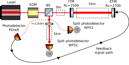
Refer to caption — Figure 1: Schematic of the test setup modelled throughout the document: a linear optical cavity is used with input laser, EOM and several photo detectors to investigate the wavefront sensing signals in the case of thermal distortion of the input mirror ITM.

The basic setup is a linear Fabry Perot cavity and a phase modulated input beam. The reflected light is detected by two wavefront sensors (WFSs). WFS1 is located directly at the input mirror’s front surface, a second beam is directed via a pick-off mirror, a lens and a 5 km distance towards WFS2. The setup is shown in figure 1 and the main parameters are given in table 1.

laser power

P=1

laser wavelength

\lambda=1064

EOM frequency

f=9

MHz

EOM modulation depth

m=0.001

(as in

\phi(t)=m\cos(\omega_{m}t)

)

ITM

Rc=2500\,{\mathrm{m}},R=98\%

T=2\%

ETM

Rc=2700\,{\mathrm{m}},R=99.9\%

T=0.1\%

cavity length

L=5\,km

Table 1: Basic parameters of the test setup

3 Field amplitudes for the aligned and resonant case

In order to confirm that the test setup as described above has been implemented correctly we record the amplitude or power of the light fields in several locations, see table 2.

		Finesse	Analytic	OSCAR
sideband amplitude after EOM	[ $\sqrt{\rm W}$ ]	$5\cdot 10^{-4}$	$5\cdot 10^{-4}$	$5\cdot 10^{-4}$
intra-cavity power	[W]	89.92	89.92	89.92
intra-cavity carrier amplitude	[ $\sqrt{\rm W}$ ]	9.483	9.483	9.483
WFS1 carrier amp.	[ $\sqrt{\rm W}$ ]	0.4528	0.4528	0.4528
WFS1 upper amp.	[ $\sqrt{\rm W}$ ]	2.5 $\,\cdot 10^{-4}$	2.5 $\,\cdot 10^{-4}$	2.5 $\,\cdot 10^{-4}$
WFS1 lower amp	[ $\sqrt{\rm W}$ ]	2.5 $\cdot 10^{-4}$	2.5 $\cdot 10^{-4}$	2.5 $\cdot 10^{-4}$
WFS2 carrier amp	[ $\sqrt{\rm W}$ ]	0.4528	0.4528	0.4528
WFS2 upper amp.	[ $\sqrt{\rm W}$ ]	2.5 $\cdot 10^{-4}$	2.5 $\cdot 10^{-4}$	2.5 $\cdot 10^{-4}$
WFS2 lower amp.	[ $\sqrt{\rm W}$ ]	2.5 $\cdot 10^{-4}$	2.5 $\cdot 10^{-4}$	2.5 $\cdot 10^{-4}$

Table 2: Light powers and field amplitudes in various locations of the optical layout.

4 Longitudinal error signal for small mirror offset

As a first test of sensing and control signals we investigate the behavior of a Pound-Drever-Hall sensing: The ETM is moved off-resonance by $0.1$ nm. We compute the error signal from the photo diode located in front of ITM, demodulated at 9 MHz, in the I-quadrature (defined by maximum signal). Finesse and OSCAR results for demodulated signals are multiplied by 2 to compensate the built-in ‘mixer gain’ of 0.5.

		Finesse	Analytic	OSCAR
Circulating power	[W]	88.8178		88.8176
LSC demodulation phase	[deg]	0.7574	-0.7574	90.7552
LSC signal in I phase (maximised)	[W]	$1.0484\cdot 10^{-4}$	$1.0484\cdot 10^{-4}$	$1.0483\cdot 10^{-4}$
LSC signal in Q phase	[W]	$1.4548\cdot 10^{-12}$	$1.3587\cdot 10^{-20}$	$-9.598\cdot 10^{-12}$

Table 3: Length sensing and control signal (LSC) taken at WFS1 position.

5 Tilt of optical fields for small mirror misalignment

Before we start computing wavefront sensor (WFS) signals, we want to make sure that the tilt of the carrier and the sideband fields are as expected.

5.1 Wavefront tilt

Compute the tilt of the wavefront on both WFSs as follows:

\phi_{\rm tilt}=\phi_{\rm sb}-\phi_{\rm carier}

(1)

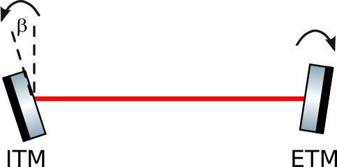
with $\phi$ being the phase of the respective field as the function of position on the WFS. Compute the slope of this for both WFSs, for the upper and lower sideband, using a) a misalignment of ITM by 0.1 nrad and b) a misalignment of ETM by 0.1 nrad. The tilt of the wavefront at the mirrors itself should be given by

2k\frac{180\,\mathrm{deg}}{\pi}\,0.1\,\mathrm{nrad}=6.7669173\cdot 10^{-2}\,\mathrm{deg/m}

(2)

Finesse results are for vertical misalignments (pitch) as discussed at the workshop, to avoid sign flips upon reflection.

a) ITM tilt
Finesse Analytic OSCAR WFS1, upper sb - carrier deg/m $7.2752\cdot 10^{-2}$ $7.2752\cdot 10^{-2}$ $\pm 0.062$ % $7.2778\cdot 10^{-2}$ WFS1, lower sb - carrier deg/m $7.1301\cdot 10^{-2}$ $7.1301\cdot 10^{-2}$ $\pm 0.067$ % $7.1339\cdot 10^{-2}$ WFS2, upper sb - carrier deg/m $-1.5698\cdot 10^{-3}$ $-1.5698\cdot 10^{-3}$ $\pm 0.110$ % $-1.5572\cdot 10^{-3}$ WFS2, lower sb - carrier deg/m $-1.2906\cdot 10^{-4}$ $-1.2909\cdot 10^{-4}$ $\pm 3.600$ % $-1.2981\cdot 10^{-4}$

b) ETM tilt
Finesse Analytic OSCAR WFS1, upper sb - carrier deg/m $-1.8428\cdot 10^{-3}$ $-1.8429\cdot 10^{-3}\pm 0.120$ % $-1.8769\cdot 10^{-3}$ WFS1, lower sb - carrier deg/m $-1.5149\cdot 10^{-4}$ $-1.5154\cdot 10^{-4}\pm 4.300$ % $-2.0131\cdot 10^{-4}$ WFS2, upper sb - carrier deg/m $-6.9613\cdot 10^{-2}$ $-6.9613\cdot 10^{-2}\pm 0.061$ % $-6.9623\cdot 10^{-2}$ WFS2, lower sb - carrier deg/m $-7.1043\cdot 10^{-2}$ $-7.1043\cdot 10^{-2}\pm 0.056$ % $-7.1046\cdot 10^{-2}$

Table 4: Wavefront tilt for the beams for an ITM or ETM misalignment of 0.1 nrad. Measurements taken at the two wavefront sensor positions. The Finesse values have been computed as an average over one beam diameter. The analytic values are means along the misaligned (yaw) axis and the errors quoted represent the largest or smallest slope across the beam - out to

20~{}cm

each side (this is the size of the virtual photodiode). Errors on wavefront tilt at the center of the beam are much smaller.

5.2 Beam propagation tilt

We can also estimate the tilt of the optical fields by comparing the beam centers at two locations on the optical axis. For this we compute the beam center on the WFSs and at temporary detectors, located (without any optical components in the path) 1 km behind the respective WFS. The beam center is estimated computing the ‘center of mass’ of the beam intensity on the detectors. The results are shows in table 5

			Finesse	OSCAR
ITM tilt	WFS1	[nrad]	-2.390	-2.356
ITM tilt	WFS2	[nrad]	2.423	2.363
ETM tilt	WFS1	[nrad]	2.833	2.790
ETM tilt	WFS2	[nrad]	-2.848	-2.783

Table 5: Beam tilt of the carrier measured at WFS1 and WSF2 (based on the beam shift over 1 km propagation).

6 Wavefront sensor signal for mirror misalignment

Now we compute the I and Q quadrature of WFS1 and WFS2 for the same misalignments as above. The optimised demodulation phases are shown in table 6.

	Finesse	Analytic	OSCAR
WFS1, demodulation phase [deg]	0.9859297	-0.985930287636	90.98173
WFS2, demodulation phase [deg]	-36.3705156	36.370514867850581	-126.4576

Table 6: Demodulation phase for the WFSs. They have been set as to maximise the ITM signal on WFS1 and the ETM signal on WFS2.

Setting these phases we can the compute an alignment sensing matrix, the Finesse results are:

\begin{pmatrix}\mathrm{WFS1}\\ \mathrm{WFS2}\end{pmatrix}=\begin{pmatrix}144.71&-2.0033\\ -1.849&-153.09\\ \end{pmatrix}\cdot\begin{pmatrix}\mathrm{ITM}\\ \mathrm{ETM}\end{pmatrix}

(3)

A preliminary, analytically derived sensing matrix was computed as:

\begin{pmatrix}\mathrm{WFS1}\\ \mathrm{WFS2}\end{pmatrix}=\begin{pmatrix}144.4123&-1.9992\\ -1.8457&-152.823\\ \end{pmatrix}\cdot\begin{pmatrix}\mathrm{ITM}\\ \mathrm{ETM}\end{pmatrix}

(4)

The discrepancy was shown to be due to numerical integration limitations in MATLAB. A grid with 5x higher resolution in both dimensions resulted in the following result:

\begin{pmatrix}\mathrm{WFS1}\\ \mathrm{WFS2}\end{pmatrix}=\begin{pmatrix}144.6978&-2.0032\\ -1.8489&-153.0803\\ \end{pmatrix}\cdot\begin{pmatrix}\mathrm{ITM}\\ \mathrm{ETM}\end{pmatrix}

(5)

which is much closer to the Finesse result.

The sensing matrix computed with OSCAR yields:

\begin{pmatrix}\mathrm{WFS1}\\ \mathrm{WFS2}\end{pmatrix}=\begin{pmatrix}144.73&-1.9703\\ -1.8905&-153.10\\ \end{pmatrix}\cdot\begin{pmatrix}\mathrm{ITM}\\ \mathrm{ETM}\end{pmatrix}

(6)

6.1 Large misalignments

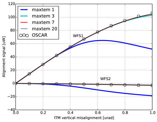
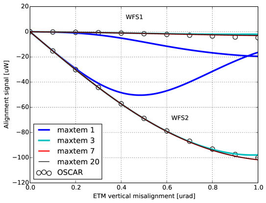
One of the more interesting tests is to model the wavefront sensor (WFS) signals for larger misalignments. In this regime especially the modal model is used outside the most simple approximation so that this represents a much more generic and more meaningful test. This test could not easily be performed with the analytic code. The comparison between Finesse ¹¹1Please note that these Finesse results require the new ‘split detector’ definition is the kat.ini as described in Appendix B. and OSCAR is shown in figure 3. The modal model converges quickly and the results from OSCAR and Finesse agree very well for misalignments below 0.4 nrad, and show a small but systematic difference for higher misalignments.

7 Thermal lens

The next step is to compute the alignment signals in the presence of a thermal lens in the ITM substrate. We assume the input mode to be the same as before the ITM thermal lens is introduced, therefore we must consider a mode mismatch between the input mode and the cavity eigenmode.

In order to verify the optical setup we assume a 100% reflective ITM and compare the beam sizes of the wavefront sensors:

	lens	Finesse	OSCAR
WFS1	50 km	6.37232 cm	6.37364 cm
WFS1	5 km	6.37232 cm	6.37499 cm
WFS2	50 km	8.09539 cm	8.09608 cm
WFS2	5 km	19.3008 cm	19.3031 cm

Table 7: Beam sizes on the wavefront senors for a thermal lens in the ITM (and assuming a 100% reflective ITM).

7.1 Beam propagation tilt with thermal lens

Similar to section 5.2 we estimate the tilt of the optical fields using a ‘center of mass’ computation. The results in table 8 show differences between OSCAR and Finesse. The reasons for that are not clear to us. Consistency checks were done with Finesse and OSCAR and did not reveal any information on which code produces more accurate results.

	lens [km]			Finesse	OSCAR
ITM tilt	50	WFS1	[nrad]	-2.366	-1.763
ITM tilt	50	WFS2	[nrad]	2.309	2.027
ETM tilt	50	WFS1	[nrad]	2.883	2.262
ETM tilt	50	WFS2	[nrad]	-2.801	-2.823
ITM tilt	5	WFS1	[nrad]	-0.843	-0.625
ITM tilt	5	WFS2	[nrad]	2.043	0.737
ETM tilt	5	WFS1	[nrad]	0.952	0.509
ETM tilt	5	WFS2	[nrad]	-2.893	-1.32

Table 8: Beam tilt of the carrier measured at WFS1 and WSF2, now with thermal lens in the ITM (Finesse results have been obtained with maxtem 8 for the 50 km lens and maxtem 29 for the 5 km lens).

7.2 Manually setting the beam parameter in Finesse

The input mode was previously automatically matched to the cavity eigenmode using the cav command in Finesse, but in order the simulate the mode mismatch we must manually set the input mode parameters using the gauss command.

In addition we might consider setting a beam parameter at the pick-off beam splitter: With the input mode and the cavity eigenmode not matched, there is no beam parameter in which the light returning from the cavity can be described as a fundamental beam. Thus higher-order modes are necessary to describe the reflected beam. Especially the thermal lens of 5 km poses a challenge as the beam parameters of the input beam (assuming for a moment a fully reflective ITM) and that of the cavity eigenmode (transmitted through the ITM) differ strongly. Measuring these beam parameters at the pick-off beam splitter yields:

•

beam parameter of reflected input beam: $w_{0}=6.37$ cm, $z<1$ mm
•

beam parameter of cavity eigenmode: $w_{0}=1.3$ cm, $z=2.395$ km

From the section ‘Limits to the paraxial approximation’ in the Finesse manual we expect this system to be outside the range in which simple paraxial models can be used. By manually setting a beam parameter ( $w_{0}=2.8$ cm, $z=1.677$ km) at the pick-off beam splitter as a compromise between the parameters measured above we can reduce the mode-mismatch in the calculation. This method has been used to compute the data shown in figure 4 and in the following.

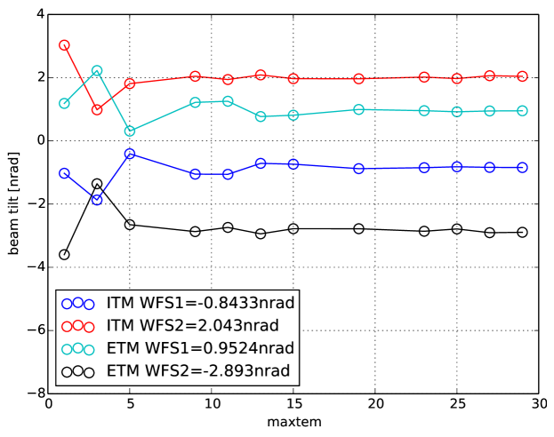
7.3 Wavefront sensor signal with thermal lens

Next we calculate the sensing matrix for small misalignments as before, but now in the presence of the thermal lens. The mode mismatch causes coupling into a wider range of higher-order modes than before, so it is necessary to use a high maxtem value. In order to check this, we calculate the sensing matrix for a range of maxtem values and look for convergence (see figures 5 and 6). For the 50 km lens case, convergence is reached by maxtem 7 or so, the 5 km lens requires at least maxtem 15.

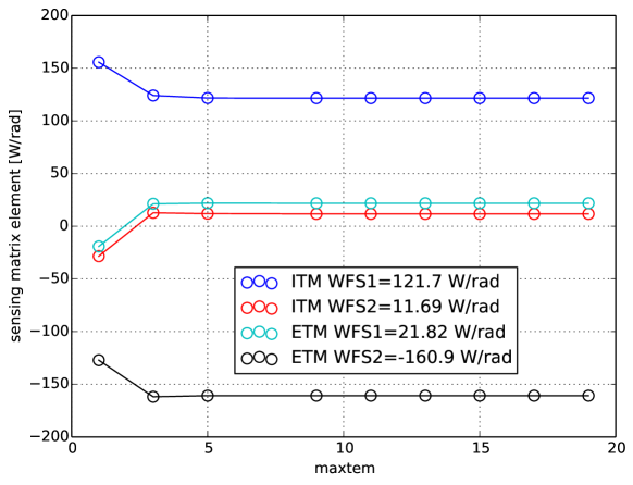
7.3.1 50 km lens in the ITM substrate

Sensing matrix computed with Finesse:

\begin{pmatrix}\mathrm{WFS1}\\ \mathrm{WFS2}\end{pmatrix}=\begin{pmatrix}121.7&21.82\\ 11.69&-160.9\\ \end{pmatrix}\cdot\begin{pmatrix}\mathrm{ITM}\\ \mathrm{ETM}\end{pmatrix}

(7)

Results obtained with OSCAR:

\begin{pmatrix}\mathrm{WFS1}\\ \mathrm{WFS2}\end{pmatrix}=\begin{pmatrix}121.98&21.50\\ 11.51&-160.55\\ \end{pmatrix}\cdot\begin{pmatrix}\mathrm{ITM}\\ \mathrm{ETM}\end{pmatrix}

(8)

Results obtained with the analytic code:

\begin{pmatrix}\mathrm{WFS1}\\ \mathrm{WFS2}\end{pmatrix}=\begin{pmatrix}121.71&21.74\\ 11.65&-160.78\\ \end{pmatrix}\cdot\begin{pmatrix}\mathrm{ITM}\\ \mathrm{ETM}\end{pmatrix}

(9)

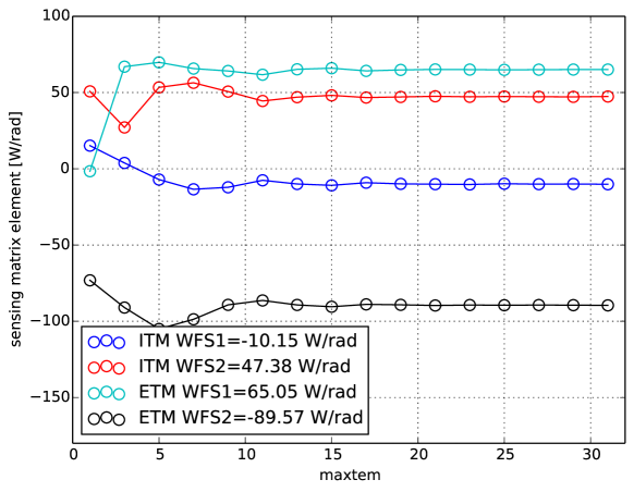
7.3.2 5 km lens in the ITM substrate

Now we compute the alignment sensing matrix with a 5 km thermal lens in the ITM substrate. This is approximately the maximum focal power that can be expected in the uncompensated aLIGO ITM.

Sensing matrix computed with Finesse at maxtem 31:

\begin{pmatrix}\mathrm{WFS1}\\ \mathrm{WFS2}\end{pmatrix}=\begin{pmatrix}-10.15&65.05\\ 47.38&-89.57\\ \end{pmatrix}\cdot\begin{pmatrix}\mathrm{ITM}\\ \mathrm{ETM}\end{pmatrix}

(10)

Results obtained with OSCAR:

\begin{pmatrix}\mathrm{WFS1}\\ \mathrm{WFS2}\end{pmatrix}=\begin{pmatrix}-0.309&54.96\\ 38.46&-126.62\\ \end{pmatrix}\cdot\begin{pmatrix}\mathrm{ITM}\\ \mathrm{ETM}\end{pmatrix}

(11)

Results obtained with the analytic code:

\begin{pmatrix}\mathrm{WFS1}\\ \mathrm{WFS2}\end{pmatrix}=\begin{pmatrix}-13.43&68.35\\ 50.94&-94.31\\ \end{pmatrix}\cdot\begin{pmatrix}\mathrm{ITM}\\ \mathrm{ETM}\end{pmatrix}

(12)

7.3.3 Conclusion

The results summarized in table 9 show some significant differences between the different methods, especially the OSCAR results include matrix elements which are different by more than a factor of 3. This is not very surprising though because already the results for the beam propagation tilt with a 5 km thermal lens showed similarly large differences. Unfortunately we do not have a reference result and thus do not know if one of the three results is correct.

	50 km lens				5 km lens
	WFS1		WFS2		WFS1		WFS2
	ITM	ETM	ITM	ETM	ITM	ETM	ITM	ETM
Finesse	121.70	21.82	11.69	-160.90	-10.15	65.05	47.38	-89.57
OSCAR	121.98	21.50	11.51	-160.55	-0.31	54.96	38.46	-126.62
Analytic	121.71	21.74	11.65	-160.78	-13.43	68.35	50.94	-94.31

Table 9: Summary table, showing all sensing matrix elements as computed will three different methods for the 50 km lens and for the 5 km lens.

References

[1] A. Freise, G. Heinzel, H. Lück, R. Schilling, B. Willke, and K. Danzmann: “Frequency-domain interferometer simulation with higher-order spatial modes”, Class. Quantum Grav. 21, S1067 (2004), the program is available at http://www.gwoptics.org/finesse
[2] K. Dooley et al.: “Report from the LLO Commissioning Workshop - January 2013”, LIGO-T1300497 (2013)
[3] J. Degallaix: “OSCAR, an optical FFT code to simulate Fabry Perot cavities with arbitrary mirror profiles” (2008), http://www.mathworks.com/matlabcentral/fileexchange/20607
[4] C. Bond, A. Freise: “Simtools, a collection of Matlab tools for optical simulations” (2013), http://www.gwoptics.org/simtools/
[5] D.Brown: “PyKat, a free Python interface and set of tools to run Finesse” (2014), http://www.gwoptics.org/pykat/

Appendix A Finesse files

All the Finesse results presented in this document have been computed starting with the base file shown below. For each simulation the extra detectors and commands have been added using a set of script files. This approach has the advantage of creating a track record of the entire process: all the results shown in this document can be reproduced at any given time, simply by re-running the scripts. The script files contain (and thus document) all changes to the Finesse input file as well as any post-processing of the results.

Originally the scripts had been written in Matlab, using the Simtools package [4]. Recently we have developed the Python package PyKat [5] which provides a more powerful and effective way to write script files for running Finesse simulations. A new set of PyKat scripts provided all the results shown in this document has been created and is available as an example in the PyKat package itself. PyKat can be downloaded at http://www.gwoptics.org/pykat.

The base file containing the main optical setup:

l psl 1.0 0 npslmod EOM 9M 0.001 1 pm 0 npsl nEOM1s s1 0 nEOM1 npo1bs1 po 0.5 0 0 45 npo1 dump npo2 nWFS1 % 50:50 pick-off mirrors s2 0 npo2 nL1lens ITM_TL 10000G nL1 nL2 % thermal lens in ITMs ITMsub 0 nL2 nITM1m1 ITM 0.02 0 0 nITM1 nITM2attr ITM Rc -2500s s_cav 5000 nITM2 nETM1m1 ETM 0.001 0 0 nETM1 nETM2attr ETM Rc 2700cav c1 ITM nITM2 ETM nETM1s spo1 1n nWFS1 nL1_inlens L1 1250 nL1_in nL1_outs spo2 5000 nL1_out nWFS2phase 0

Appendix B Split detectors definition in the kat.ini file of Finesse

During the simulation workshop we realised that the definition of split detectors (WFS) in the default kat.ini file distributed with Finesse until version 1.0 was not correct. The original definition looks as follows:

PDTYPE y-splitx 0 x 1 1.0x 0 x 3 1.0x 0 x 5 1.0x 0 x 7 1.0x 0 x 9 1.0x 0 x 11 1.0x 0 x 13 1.0x 0 x 15 1.0x 2 x 1 1.0x 2 x 3 1.0x 2 x 5 1.0x 2 x 7 1.0x 2 x 9 1.0x 2 x 11 1.0x 2 x 13 1.0x 2 x 15 1.0x 4 x 1 1.0x 4 x 3 1.0x 4 x 5 1.0x 4 x 7 1.0x 4 x 9 1.0...

In order to continue this document a correct sequence of beat coefficients has been derived and is available now. The derivation is described in the new Finesse manual and the resulting coefficients list begins like this:

PDTYPE y-splitx 0 x 1 0.797884560802865x 0 x 3 -0.32573500793528x 0 x 5 0.218509686118416x 0 x 7 -0.168583882836184x 0 x 9 0.139074607877595x 0 x 11 -0.119342192152758x 0 x 13 0.105105246952603x 0 x 15 -0.0942883643366146x 2 x 1 0.564189583547756x 2 x 3 0.690988298942671x 2 x 5 -0.257516134682126x 2 x 7 0.166889529453113x 2 x 9 -0.126437912127138x 2 x 11 0.103140489653528x 2 x 13 -0.0878334751963773x 2 x 15 0.0769291636262473x 4 x 1 -0.16286750396764x 4 x 3 0.598413420602149x 4 x 5 0.669046543557288x 4 x 7 -0.240884286886713x 4 x 9 0.153297821464995...