Spin relaxation of a diffusively moving carrier in a random hyperfine field

Abstract

Relaxation, $\langle S_{z}(t)\rangle$, of the average spin of a carrier in course of hops over sites hosting random hyperfine fields is studied theoretically. In low dimensions, $d=1,2$, the decay of average spin with time is non-exponential at all times. The origin of the effect is that for $d=1,2$ a typical random-walk trajectory exhibits numerous self-intersections. Multiple visits of the carrier to the same site accelerates the relaxation since the corresponding partial rotations of spin during these visits add up. Another consequence of self-intersections of the random-walk trajectories is that, in all dimensions, the average, $\langle S_{z}(t)\rangle$, becomes sensitive to a weak magnetic field directed along $z$. Our analytical predictions are complemented by the numerical simulations of $\langle S_{z}(t)\rangle$.

Introduction. One of the reasons why organic semiconductors are promising candidates for the active layers of spin valvesv1 ; v2 ; v3 ; v4 ; v5 is a long spin lifetime, $\tau_{s}$, in these materials. Due to long $\tau_{s}$, spin-polarized carriers, injected from one ferromagnetic electrode into the active layer, preserve their spin orientation while traveling towards the other ferromagnetic electrode. As a result, the resistance of the device depends on the mutual orientations of magnetizations of the electrodes (the spin-valve effect). The origin of slow spin relaxation in organic semiconductors is that they are composed from light atoms with weak spin-orbit coupling.

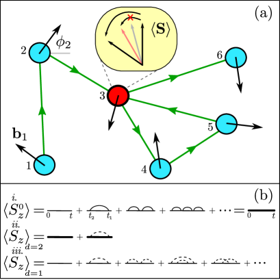
Figure 1: (Color online) (a) In course of diffusion $1\rightarrow 2\rightarrow 3\rightarrow 4\rightarrow 5\rightarrow 3\rightarrow 6$ over sites hosting random hyperfine fields (black arrows) a carrier visits the site $3$ twice. As a result, the partial spin rotation doubles, see enlargement; (b) i. For a trajectory without self-intersections $\langle S_{z}(t)\rangle$ is given by sequence of non-intersecting solid arcs encoding the correlator $C_{0}$, ii. Graphical representation of Eq. (11) for the $d=2$ spin relaxation; self-intersections are captured by a single dashed arc encoding the correlator $C_{D}$, iii. Spin relaxation for $d=1$ is described by diffusive diagrams only.

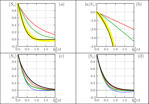
Figure 2: (Color online) (a) $d=2$ spin relaxation for uncorrelated (no self-crossings) hyperfine fields ${\bm{b}}_{i}$ (red), with self-intersections and spherically distributed ${\bm{b}}_{i}$ (green), and with self-intersections and planar ${\bm{b}}_{i}$ (black); (b) Same as (a) but in log-scale. The decay $\langle S_{z}(t)\rangle$ is a simple exponent (red), shows crossover between two simple exponents (green), strongly non-exponential (black). Yellow line is plotted from Eq. (11) with $g_{\scriptscriptstyle 2}=0.75$; (c) and (d): weak external field $B\sim\tau_{s}^{-1}$ suppresses the effect of self-intersections. Numerical (c) and analytical (d) results illustrate how a simple-exponent decay is restored upon increasing $B\tau_{s}$. Results for $B=0$ (blue), $B\tau_{s}=2$ (green), $B\tau_{s}=5$ (red), and $B\tau_{s}=10$ (black) are shown.

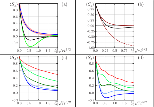
Figure 3: (Color online) For $d=1$ random walk the decay, $\langle S_{z}(t)\rangle$, is a universal function of $b_{0}^{2}\sqrt{\tau}t^{3/2}$. (a) numerical results for a planar hyperfine field (black) exhibit spin reversal at intermediate time. For a spherically distributed ${\bm{b}}_{i}$ (blue) the decay is monotonic but non-exponential and is accurately captured by the solution of the self-consistent equation Eq. (18) (pink). Green curve is the numerical solution of Eq. (18) for planar hyperfine field. (b) Black curve is the same as in (a), while brown and dashed brown show the result of partial summation of the diffusive diagrams, see text. Weak external field slows down the decay of $\langle S_{z}(t)\rangle$ for both spherical (c) and planar ${\bm{b}}_{i}$ (d). Numerical results are shown for the following values of $\frac{B}{b_{0}^{4/3}\tau^{1/3}}$: $0$ (dark blue), $1$ (light blue), $2$ (dark green), $4$ (light green), and $8$ (red).

In the absence of spin-orbit coupling, the leading mechanism of the spin memory loss is a precession of spin in random hyperfine fields created by surrounding protons on the sites visited by the carrier in course of traveling between the electrodes. With mobility in organic semiconductors being very low, the charge transport in them is via random inelastic hops of carriers between the sites. Then the waiting time, $\tau$, for a subsequent hop plays the role of the correlation time for the random magnetic field, with rms $b_{0}$, acting on the carrier spin. As a result, the Dyakonov-Perel expressionDP1971 for $\tau_{s}$ assumes the form

$$\tau_{s}=\frac{1}{b_{0}^{2}\tau}.$$ (1)

Naturally, for long $\tau_{s}$, a typical partial rotation of spin, $\delta\varphi=b_{0}\tau$, during the waiting time is weak, $\delta\varphi\ll 1$. Assuming that all partial rotations are completely uncorrelated, the spin polarization, averaged over realizations of the hyperfine fields, falls off with the number of hops, $N$, as $\langle S_{z}(N)\rangle=S_{z}(0)\exp\left(-N\delta\varphi^{2}\right)$. This suggests that the evolution of $\langle S_{z}\rangle$ with time $t=N\tau$ is a simple exponent

$$\langle S_{z}(t)\rangle=S(0)\exp\Bigl{(}-\frac{t}{\tau_{s}}\Bigr{)}.$$ (2)

The main message of the present paper is that the random walk of a carrier over the sites induces the correlation in hyperfine fields “sensed” by the carrier spin. This correlation modifies the decay law Eq. (2). The origin of correlation is the self-intersections of the random-walk trajectories, see Fig. 1. These self-intersections imply multiple visits of the carrier to the same site. Then the corresponding partial rotations add up which leads to acceleration of the spin relaxation. The effect is most dramatic if the carrier moves in one dimension. Then, in course of $N$ hops, the carrier visits $N^{1/2}$ sites, and the number of visits to a given site is also $N^{1/2}$. The $N$-dependence of $\langle S_{z}\rangle$ can be found from the above derivation of Eq. (2) upon replacement $N\rightarrow N^{1/2}$ and $\delta\varphi\rightarrow N^{1/2}\delta\varphi$. This yields $\langle S_{z}(N)\rangle=S_{z}(0)\exp\left(-N^{3/2}\delta\varphi^{2}\right)$, and, correspondingly, the time dependence

$$\langle S_{z}(t)\rangle=S(0)\exp\Bigl{(}-\frac{t^{3/2}}{\tau^{1/2}\tau_{s}}\Bigr{)}.$$ (3)

In higher dimensions, $d=2$ and $d=3$, the number of self-crossings of an $N$-step random-walk trajectory is $\sim N$ and $\sim N^{1/2}$, respectively, i.e. each site is visited twice with probability $\sim 1$ for $d=2$, and with probability $N^{-1/2}$ for $d=3$. As a result, the change, $\langle\delta S_{z}(t)\rangle$, of the decay law Eq. (2) due to accumulation of the partial rotations is of the order of $\langle S_{z}(t)\rangle$ for $d=2$ and of the order of $\left(\tau/t\right)^{1/2}\langle S_{z}(t)\rangle$ for $d=3$. But even in the latter case the correction to Eq. (2) can be important since it induces a sensitivity of $\langle S_{z}(t)\rangle$ to a weak external magnetic field directed along $z$. Recall that, without self-intersections, the $B$-dependence of $\tau_{s}$ is given by the Hanle-type expression

$$\tau_{s}=\frac{1+B^{2}\tau^{2}}{b_{0}^{2}\tau},$$ (4)

which applies for $B\gg b_{0}$ and predicts that sensitivity to $B$ emerges at $B\sim\tau^{-1}\gg b_{0}$. We will demonstrate that, with self-crossings of the random-walk trajectories taken into account, the sensitivity to $B$ develops at much smaller field $B\sim(\tau\tau_{s}^{2})^{-1/3}\ll\tau^{-1}$ in one dimension and at $B\sim\tau_{s}^{-1}\ll\tau^{-1}$ for $d=2$ and $d=3$. Remarkably, the returns to the same site after a long time, $t$, give rise to the oscillatory correction $\propto\cos Bt$ to $\langle S_{z}(t)\rangle$, which is most pronounced for $d=1$.

Diagrammatic expansion. To illustrate our main message, consider first a simplified situation, when the hyperfine field is located in the $x,y$-plane. Moreover, we will assume that the randomness in the in-plane field, $b_{\perp}=(b_{x},b_{y})$, is exclusively due to randomness in the azimuthal angle $\phi$, i.e. $b_{x}=b_{0}\cos\phi$, $b_{y}=b_{0}\sin\phi$, see Fig. 1.

The spin operator satisfies the equation of motion $i\frac{d\widehat{S}}{dt}=[\widehat{S},\widehat{H}]$, with Hamiltonian $\widehat{H}=\widehat{S}\cdot{\bm{b}}(t)$. Excluding the in-plane components of the operator $\widehat{S}$, the equation of motion for $S_{z}$ takes the form

$$S_{z}(t)=1-b_{0}^{2}\int\limits_{0}^{t}dt_{1}\int\limits_{0}^{t_{1}}dt_{2}\;\cos(\phi(t_{1})-\phi(t_{2}))S_{z}(t_{2}).$$ (5)

To find the time evolution of the average, $\langle S_{z}(t)\rangle$, it is necessary to iterate Eq. (5) as

$$S_{z}(t)=1-b_{0}^{2}\int\limits_{0}^{t}dt_{1}\int\limits_{0}^{t_{1}}dt_{2}\cos(\phi(t_{1})-\phi(t_{2}))+b_{0}^{4}\int\limits_{0}^{t}dt_{1}\int\limits_{0}^{t_{1}}\,\,dt_{2}\int\limits_{0}^{t_{2}}dt_{3}\int\limits_{0}^{t_{3}}dt_{4}\cos(\phi(t_{1})-\phi(t_{2}))\cos(\phi(t_{3})-\phi(t_{4}))-\cdots$$ (6)

and perform averaging over the random azimuthal angle, $\phi(t)$. Without self-intersections of the random-walk trajectories, this averaging is straightforward since the angles $\phi(t)$, $\phi(t^{\prime})$ are correlated only for $|t-t^{\prime}|\lesssim\tau\ll t$, i.e.

$$\langle\cos(\phi(t)-\phi(t^{\prime}))\rangle=\exp\left[-|t-t^{\prime}|/\tau\right]=C_{0}(t,t^{\prime}).$$ (7)

The exponential character of $C_{0}$ expresses the Poisson distribution of the waiting times.

Each term of the expansion Eq. (6) can be graphically expressed as a diagram, see Fig. 1. Because of the short-time decay of $C_{0}$, the arcs corresponding to $C_{0}$ terms are not allowed to cross. More precisely, each crossing of arcs gives rise to a small factor $\tau/t\ll 1$. On the other hand, averaging of each term with $n$ non-intersecting arcs yields $(-1)^{n}(b_{0}\tau)^{2n}/n!$, and we restore Eq. (2).

As a consequence of self-intersections of the random-walk path, the difference $(\phi(t)-\phi(t^{\prime}))$ can be small even if the moments $t$ and $t^{\prime}$ are well separated in time. Quantitatively, this is captured by the diffusive contribution, $C_{D}$, to the correlator

$$\langle\cos(\phi(t)-\phi(t^{\prime}))\rangle=\left[\frac{1}{2\pi D|t-t^{\prime}|}\right]^{d/2}=C_{D}(t,t^{\prime}),$$ (8)

where the diffusion coefficient $D$ is $1/\tau$ assuming that the separation between neighboring sites is unity. In Eq. (8), self-intersections are accounted for in the continuous limit as a probability to return to the origin after moving diffusively for a time $t^{\prime}-t$.

The correlator $C_{D}$ should also be incorporated into the diagrammatic expansion; we denote it with dashed arcs, see Fig. 1. For example, the diagram involving only one dashed arc is given by

$$\lambda_{d}(t)=b_{0}^{2}\int\limits_{0}^{t}dt_{1}\int\limits_{0}^{t_{1}}dt_{2}\left[\frac{1}{2\pi D\left|t_{1}-t_{2}\right|}\right]^{d/2}.$$ (9)

Evaluation of the double integral yields

$$\lambda_{d}(t)=\left\{\begin{matrix}\dfrac{4}{3(2\pi)^{1/2}}\dfrac{t^{3/2}}{\sqrt{\tau}\tau_{s}},&d=1,\\ \dfrac{1}{2\pi\tau_{s}}\left[t\ln\left(\dfrac{t}{\tau}\right)\right],&d=2,\\ \dfrac{2\tau^{1/2}}{(2\pi)^{3/2}\tau_{s}}\left(\dfrac{t}{\sqrt{\tau}}-2\sqrt{t}\right),&d=3,\end{matrix}\right.$$ (10)

where we have expressed $b_{0}^{2}$ in terms of $\tau_{s}$ and have taken into account that the diffusive description applies when $t_{1}-t_{2}\gtrsim\tau$. The double integral, Eq. (9) converges for $d=1$ and the result, Eq. (10), confirms the qualitative argument given in the Introduction. Namely the averaged expansion Eq. (6) becomes a series in the dimensionless combination $b_{0}^{2}t^{3/2}\tau^{1/2}$. Note also, that for $d=1$ the diffusive contribution Eq. (9) exceeds by $(t/\tau)^{1/2}$ the contribution coming from a single solid-arc. This illustrates the fact that each site is visited many times in the course of a $d=1$ random walk.

In two dimensions, the contribution $\lambda_{2}(t)$, to $\langle S_{z}(t)\rangle$ from a dashed arc exceeds logarithmically the contribution from one solid arc. On the other hand, this contribution contains a prefactor $(2\pi)^{-1}$. We will take advantage of the smallness of this prefactor and sum up all diagrams containing only zero or one dashed arc, as illustrated in Fig. 1b. The most delicate ingredient of this procedure is that the insertion of solid arcs under a dashed arc amounts to the replacement $C_{D}(t_{1},t_{2})\rightarrow C_{D}(t_{1},t_{2})\exp\left[-\frac{(t_{2}-t_{1})}{2\tau_{s}}\right]$. Physically, this means that between the two subsequent visits to the same site at time moments $t_{1}$ and $t_{2}$, the spin polarization is “forgotten” in the course of many short-time hops. The emergence of the non-trivial factor $1/2$ in the exponent is demonstrated in the Supplemental MaterialSupplemental where we also show that the presence of a $z$-component of the hyperfine field amounts to the replacement $C_{D}(t_{1},t_{2})\rightarrow C_{D}(t_{1},t_{2})\exp\left[-\frac{3(t_{1}-t_{2})}{4\tau_{s}}\right]$.

For planar hyperfine fields the resulting expression for $\langle S_{z}(t)\rangle$, which is shown graphically in Fig. 1b, takes the form

$$\langle S_{z}(t)\rangle=e^{-t/\tau_{s}}-\frac{g_{\scriptscriptstyle 2}}{2\pi\tau_{s}}e^{-t/\tau_{s}}\int\limits_{0}^{t}dt_{1}\int\limits_{\tau}^{t_{1}}dt_{2}\frac{\exp\left[-\frac{(t_{2}-t_{1})}{2\tau_{s}}\right]}{t_{1}-t_{2}},$$ (11)

where the numerical factor $g_{\scriptscriptstyle 2}$ should be $1$, but is retained intentionally for future comparison with numerics. The second term is responsible for the deviation from a simple exponential decay. This term can be easily reduced to a single integral, and we get

$$\langle S_{z}(t)\rangle=e^{-t/\tau_{s}}\left(1-\frac{g_{\scriptscriptstyle 2}}{\pi}\int\limits_{\tau/2\tau_{s}}^{t/2\tau_{s}}\!\!\frac{dw}{w}\left(\frac{t}{2\tau_{s}}-w\right)e^{w}\right).$$ (12)

For small $t\ll\tau_{s}$, Eq. (12) yields the correction, $-\frac{g_{\scriptscriptstyle 2}}{2\pi\tau_{s}}t\ln(t/\tau)$, to a simple exponent which reproduces Eq. (10). In the limit $t\gg\tau_{s}$ the correction takes the form $\frac{g_{\scriptscriptstyle 2}}{\pi}\left(\frac{\exp\left(-t/2\tau_{s}\right)}{(t/2\tau_{s})}\right)$. In fact, this asymptote applies already at $t>\tau_{s}$. It decays slower than $\exp(-t/\tau_{s})$, so that $\langle S_{z}(t)\rangle$ should exhibit a sign reversal followed by a minimum. Our numerics, see below, shows that this minimum is very shallow.

Turning now to $d=3$, we find that the first dominant term in Eq. (10) describes the contribution from short times and essentially renormalizes $\tau_{s}$. The second subleading term comes from long diffusive trajectories. It yields a correction to $\langle S_{z}(t)\rangle$ which is small as $\left(\frac{t}{\tau_{s}}\right)^{1/2}$ at $t\ll\tau_{s}$ and as $\left(\frac{\tau_{s}}{t}\right)^{3/2}\exp\left(\frac{-t}{2\tau_{s}}\right)$ at $t\gg\tau_{s}$. The importance of this correction is that it causes a sensitivity of $\langle S_{z}(t)\rangle$ to a weak external magnetic field, as we show below.

Sensitivity to the magnetic field along the $z$-axis. Incorporating the constant, ${\bm{B}}={\bm{z}}_{0}B$, and random, $b_{z}(t)$, components of the magnetic field amounts to the replacement

$$\Bigl{[}\phi(t_{1})\!-\!\phi(t_{2})\Bigr{]}\rightarrow\left[\phi(t_{1})-\phi(t_{2})+B(t_{1}\!-\!t_{2})+\int\limits_{t_{1}}^{t_{2}}dt^{\prime}b_{z}(t^{\prime})\right]$$ (13)

in Eq. (6). As discussed in the Introduction, the solid-arc diagrams describing the hops to nearest neighbors during the time intervals $\sim\tau$ develop the sensitivity to $B$ only for strong $B\sim\tau^{-1}$. On the other hand, the dashed-arc diagrams are defined by much longer times, and are thus sensitive to much weaker $B$. The most interesting domain of $B$ for $d=2,3$ is $\left(b_{0}\tau\right)^{-1}\gg\frac{B}{b_{0}}\gg\left(b_{0}\tau\right)$, where $B\tau$ is small but $B\tau_{s}$ is large. In this domain the decay of $\langle S_{z}(t)\rangle$ is predominantly exponential while the $B$-dependence comes from the diffusive correction. For $d=1$ the corresponding domain of $B$ is $\left(b_{0}\tau\right)^{-1}\gg\frac{B}{b_{0}}\gg\left(b_{0}\tau\right)^{1/3}$. Technically, in this domain, one can neglect the decoration of the diffusive propagator by solid arcs and rewrite the diffusive contribution Eq. (9) as

$$\delta\langle S_{z}(t)\rangle=-\frac{b_{0}^{2}\tau^{\frac{d}{2}}}{(2\pi)^{d/2}}\int\limits_{0}^{t}dt_{1}\int\limits_{0}^{t_{1}}dt_{2}\frac{\cos B\left(t_{1}-t_{2}\right)}{\left(t_{1}-t_{2}\right)^{d/2}}\\ =-\frac{b_{0}^{2}\tau^{\frac{d}{2}}t^{2-\frac{d}{2}}}{(2\pi)^{d/2}}F_{d}\left(Bt\right),$$ (14)

where the function $F_{d}\left(v\right)$ is defined as

$$F_{d}\left(v\right)=\int\limits_{0}^{1}dx\int\limits_{0}^{x}dy~{}\frac{\cos v(x-y)}{\left(x-y\right)^{d/2}}.$$ (15)

The form of the function, $F_{d}(v)$, suggests that the diffusive correction contains both smooth and oscillating contributions. The meaning of the smooth contribution is that, upon visiting the same site at times $t_{1}$ and $t_{2}$, partial spin rotations add up only if $|t_{1}-t_{2}|\lesssim 1/B$. The oscillatory contribution originates from their “phase shift”, $B(t_{2}-t_{1})$.

Analysis of Eqs. (14), (15) yields the following asymptotes describing the $B$-dependent correction to $\langle S_{z}(t)\rangle$

$$\left[F_{d}(v)-F_{d}(0)\right]_{v\gg 1}=\varkappa_{d}(v)-\frac{\cos v}{v^{2}},$$ (16)

where $\varkappa_{d}(v)=(\pi/2v)^{1/2}$, $-\ln(v)$, and $-(2\pi v)^{1/2}$ for $d=1,2,$ and $3$, respectively. It follows from Eq. (16) that magnetic field causes a cutoff of the diffusive correction Eq. (14), so that the value $\delta\langle S_{z}(t)\rangle$ approaches the value $\sim-b_{0}^{2}\tau^{d/2}/B^{2-d/2}$ at large times. With regard to oscillations, their amplitude falls off with time as $\left(b_{0}^{2}/B^{2}\right)(\tau/t)^{d/2}$, i.e. the oscillations are more pronounced in lower dimensions.

Numerical results. We simulated the spin evolution numerically using the discrete version of the equation of motion

$${\bm{S}}_{i}=\Bigl{[}{\bm{S}}_{i-1}-{\bm{n}}_{i}\left({\bm{n}}_{i}\cdot{\bm{S}}_{i-1}\right)\Bigr{]}\cos b_{0}\tau\\ +\left({\bm{n}}_{i}\times{\bm{S}}_{i-1}\right)\sin b_{0}\tau+{\bm{n}}_{i}\left({\bm{n}}_{i}\cdot{\bm{S}}_{i-1}\right),$$ (17)

so that the local hyperfine field had the same magnitude, $b_{0}$, on all sites, while the directions, ${\bm{n}}_{i}$, were defined by either a random azimuthal angle, $\phi_{i}$, or by two spherical angles, $\phi_{i}$ and $\theta_{i}$. The diffusive motion of a carrier was simulated by randomly choosing ${\bm{n}}_{i}$ at the next step from one of the nearest neighbors of ${\bm{n}}_{i}$ at the previous step.

Our numerical results are shown in Figs. 2 and 3. We started by verifying that, for a directed walk, when all ${\bm{n}}_{i}$ are uncorrelated, $\langle S_{z}(i)\rangle$ decays as a simple exponent. It is seen from Fig. 2 that, upon allowing self-intersections, the numerical curve $\langle S_{z}(t)\rangle$ drops below the result for uncorrelated ${\bm{n}}_{i}$ after several steps. For a spherical hyperfine field, $\ln\langle S_{z}(t)\rangle$ remains essentially linear at large $t$, but with bigger slope, i.e. the evolution of $\langle S_{z}(t)\rangle$ exhibits a crossover from one simple exponent at short times to another simple exponent at long times. By contrast, for planar hyperfine field, $\langle S_{z}(t)\rangle$ is strongly nonlinear in the log-scale at all times. This completely non-exponential decay is very well described by Eq. (12) with $g_{\scriptscriptstyle 2}=0.75$ instead of $1$.

As we argued above, self-intersections give rise to the sensitivity of the spin relaxation to magnetic field $B\sim\frac{1}{\tau_{s}}\ll\frac{1}{\tau}$. Evolution of the numerical curves with $B$ is shown in Fig. 2. A significant slowing down of the relaxation starts from $B\sim\frac{5}{\tau_{s}}$. We have also plotted an analytical dependence of $\langle S_{z}(t)\rangle$ obtained by introducing $\cos Bt(x_{1}-x_{2})$ into the integrand of Eq. (11). Qualitatively, the numerical and analytical curves exhibit similar behavior. Note however, that the analytical curves saturate at $B\tau_{s}\sim 15$, while the numerical curves flatten progressively with increasing $B$. This discrepancy is simply due to the fact that the analytical curves correspond to a vanishing product $B\tau$, and thus cannot capture the conventional spin relaxation Eq. (4). With regard to the oscillating correction $\propto\cos Bt$ predicted by Eq. (16), they show up in simulations, but their magnitude is too small to be resolved in Fig. 2.

Numerical results for random walk in one dimension are shown in Fig. 3. Firstly, we established that these numerical results perfectly satisfy the scaling relation predicted from the qualitative reasoning. Namely, when plotted versus $t^{3/2}b_{0}^{2}\tau^{1/2}$, they all fall on a single curve. We also see that the empirical prediction Eq. (3) does not apply. In fact, for purely planar hyperfine field, the numerical curve, $\langle S_{z}(t)\rangle$, drops to a negative value $\langle S_{z}\rangle\approx-0.16$ before approaching zero. As we explained above, only the dashed arcs are responsible for the spin relaxation for $d=1$. Therefore, capturing the nontrivial decay of $\langle S_{z}\rangle$ analytically, requires summation of at least a part of dashed-arc-diagrams to all orders.

In the Supplemental Material we present two variants of such summation. They essentially reduce to exponentiating of one-dashed-arc contribution, $\lambda_{1}(t)$, Eq. (9), and differ by the way the numerical factors in the diagrams with crossings are counted. Two ways of approximate counting yield $\langle S_{z}(t)\rangle=\exp\left[-\lambda_{1}(t)\right]$ and $\langle S_{z}(t)\rangle=2\exp\left[-\frac{\lambda_{1}(t)}{2}\right]-1$, which lie above and below the numerical results, see Fig. 3. An alternative approach is to sum only the contributions from non-overlapping diffusive diagrams Fig. 1. We showSupplemental that this summation leads to a self-consistent equation

$$\frac{d\langle S_{z}\rangle}{du}=-\frac{4}{9(2\pi)^{1/2}u^{1/3}}\\ \times\int_{0}^{u}\frac{du_{1}\exp\left[-\left(u^{2/3}-u_{1}^{2/3}\right)^{3/2}\right]\langle S_{z}(u_{1})\rangle}{u_{1}^{1/3}\left(u^{2/3}-u_{1}^{2/3}\right)^{1/2}},$$ (18)

where $u=b_{0}^{2}\tau^{1/2}t^{3/2}$. When the hyperfine field is planar, the numerator in Eq. (18) is $1$. Eq. (18) does not contain any parameters. Its numerical solutions for spherical and planar hyperfine fields are shown in Fig. 3. We see that for spherical case the solution closely reproduces the simulated decay of $\langle S_{z}(t)\rangle$. For planar case, the agreement of the solution with the result of simulation is less accurate. In particular, the depth of the minimum in $\langle S_{z}(t)\rangle$ predicted by the self-consistent equation is $-0.28$ instead of $-0.16$. Besides, the self-consistent equation predicts additional weak oscillations in $\langle S_{z}(t)\rangle$ at long times. Unlike $d=2$, the oscillations in $\langle S_{z}(t)\rangle$ in a finite magnetic field are clearly seen in the numerical data, Fig. 3. They develop at $B\approx b_{0}^{4/3}\tau^{1/3}$.

Discussion. Effect of returns to the origin on the spin relaxation was previously discussed in Refs. KachorovskiiSpinMemory, ; ShermanNonexponential, ; SO+1Dlocalization, . It was assumed that the mechanism of relaxation is the spin-orbit couplingDP1971 . For this mechanism, the random field “sensed” by electron depends on the direction of its velocity. Then the effect of accumulation of the spin rotation upon multiple visits to the same site, which is central to the present paper, does not apply. For a unidirectional motion there are no returns and the average spin polarization decays as a simple exponent. At the same time, the local spin polarization exhibits very strong fluctuationswe1 ; we2 . To interpret the anomalous sensitivity of $\langle S_{z}(t)\rangle$ to the external magnetic field, ${\bm{B}}={\bm{z}}_{0}B$, it is instructive to draw analogy to the anomalous sensitivity of the resistance of metals to a weak magnetic field (weak localizationWL ). Namely, the phase, $Bt$, of the spin rotation is analogous to the orbital Aharonov-Bohm phase. In weak localization, weak $B$ restricts the area within which counter-propagating random-walk trajectories interfere constructively. In spin relaxation, weak $B$ limits the time interval within which accumulation of spin rotation due to self-intersections takes place.

Acknowledgements. We are grateful to Sarah Li and Z. V. Vardeny for motivating us. We are also strongly grateful to V. V. Mkhitaryan for reading the manuscript and helpful remarks. This work was supported by the NSF through MRSEC DMR-112125.

I Supplemental material

I.1 Modification of the diffusive correlator by the short-time correlators

In order to establish how the short-time correlations modify the correlations due to self-intersections of the diffusive trajectories, consider the second term of Eq. (6). This term contains the combination

$$-\cos\bigl{(}\phi(t_{1})-\phi(t^{\prime})\bigr{)}\cos\bigl{(}\phi(t^{\prime\prime})-\phi(t_{2})\bigr{)}$$ (19)

of four azimuthal angles. Assume that the carrier visits the same site at distant times moments $t_{1}$ and $t_{2}$, while $t^{\prime}$ and $t^{\prime\prime}$ are the initial and final moments of some hop that takes place between $t^{\prime}$ and $t^{\prime\prime}$. Then the averaging over $t^{\prime}$, $t^{\prime\prime}$ should be performed using the correlator Eq. (7). To perform this averaging it is convenient to decompose the product Eq. (19) into a sum

$$-\frac{1}{2}\cos\bigl{(}\phi(t_{1})-\phi(t_{2})+\phi(t^{\prime\prime})-\phi(t^{\prime})\bigr{)}$$

$$-\frac{1}{2}\cos\bigl{(}\phi(t_{1})+\phi(t_{2})-\phi(t^{\prime})-\phi(t^{\prime\prime})\bigr{)}.$$ (20)

The second term containing the sum, $\bigl{(}\phi(t^{\prime})+\phi(t^{\prime\prime})\bigr{)}$, is zero on average. The first term contains the difference, $\bigl{(}\phi(t^{\prime})-\phi(t^{\prime\prime})\bigr{)}$, and averages to

$$-\frac{1}{2}C_{0}(t^{\prime},t^{\prime\prime})\cos\bigl{(}\phi(t_{1})-\phi(t_{2})\bigr{)}.$$ (21)

Consider now two intermediate hops taking place within the intervals $\left[t^{\prime},t^{\prime\prime}\right]$ and, subsequently, $\left[t^{\prime\prime\prime},t^{\prime\prime\prime\prime}\right]$, between the moments $t_{1}$ and $t_{2}$. The corresponding combination to be averaged over the initial and final moments of the hops reads

$$\cos\bigl{(}\phi(t_{1})-\phi(t^{\prime})\bigr{)}\cos\bigl{(}\phi(t^{\prime\prime})-\phi(t^{\prime\prime\prime})\bigr{)}$$

$$\times\cos\bigl{(}\phi(t^{\prime\prime\prime\prime})-\phi(t_{2})\bigr{)}.$$ (22)

To average over orientations of the on-site hyperfine fields we have to perform the above decomposition twice, which yields $\frac{1}{4}C_{0}(t^{\prime},t^{\prime\prime})C_{0}(t^{\prime\prime\prime},t^{\prime\prime\prime\prime})\cos\bigl{(}\phi(t_{1})-\phi(t_{2})\bigr{)}$.

Upon integration Eq. (21) over $t^{\prime}$, $t^{\prime\prime}$ within the interval $t_{1}<t^{\prime}<t^{\prime\prime}<t_{2}$, we conclude that a single hop, described by a solid arc, modifies the integrand in the expression for a diffusive arc by a factor $-\frac{1}{2}\frac{(t_{2}-t_{1})}{\tau_{s}}$. Similarly, for two hops, upon integrating over their initial and final moments, we find that they modify the integrand by a factor $\frac{1}{4}\frac{(t_{2}-t_{1})^{2}}{2!\tau_{s}}$. Adding the contributions from zero, one, two, three, etc. hops, we conclude that intermediate hops lead to the factor $\exp\left[-\frac{(t_{2}-t_{1})}{2\tau_{s}}\right]$ in the integrand.

In the above reasoning it was implicit that intermediate hops take place between the time moments $t_{1}$ and $t_{2}$. In order to calculate the correction to $\langle S_{z}(t)\rangle$ due to diffusive random walk, we also have to take into account the intermediate hops that take place outside the domain $(t_{1},t_{2})$. In a manner similar to the above, one can realize that short hops which take place during interval $(0,t_{1})$ are accounted for by multiplying $C_{D}(t_{1},t_{2})$ by the factor $\exp(-t_{1}\tau_{s})$. We emphasize that, unlike in the domain $(t_{1},t_{2})$, the argument of the exponent does not contain $1/2$. Similarly, the short hops in the domain $(t_{2},t)$ cause an additional factor $\exp[-(t-t_{2})/\tau_{s}]$. All three factors coming from short hops are taken into account in the second term in Eq. (11) of the main text.

In the presence of a $z$-component of the hyperfine field, the average Eq. (21) assumes the form

$$-\frac{1}{2}C_{0}(t^{\prime},t^{\prime\prime})\cos\bigl{(}\phi(t_{1})-\phi(t_{2})\bigr{)}\\ \times\left<\cos\left(-\int\limits_{t_{2}}^{t^{\prime\prime}}b_{z}(s)ds-\int\limits_{t^{\prime}}^{t_{1}}b_{z}(s)ds\right)\right>.$$ (23)

Recall now, that $C_{0}(t^{\prime},t^{\prime\prime})$ restricts $t^{\prime}$ and $t^{\prime\prime}$ within $\tau$ from each other. Then the argument of the cosine in Eq. (23) reduces to a single integral, $\Phi=\int\limits_{t_{2}}^{t_{1}}b_{z}(s)ds$. Averaging of this cosine over the realizations of $b_{z}$ can be performed analytically using the fact that the relevant times $t_{1}$ and $t_{2}$ are of the order of $\tau_{s}$, which is much bigger than $\tau$. Therefore, the phase, $\Phi$, contains many random contributions, which allows us to use the relation $\langle\cos\Phi\rangle=\exp\left[-\frac{1}{2}\langle\Phi^{2}\rangle\right]$. The average, $\langle\Phi^{2}\rangle$, can be expressed via $\tau_{s}$ as $\langle\Phi^{2}\rangle=\frac{(t_{2}-t_{1})}{4\tau_{s}}$. Thus we conclude that, in addition to the factor $-\frac{(t_{2}-t_{1})}{2\tau_{s}}$, a single arc brings an additional factor, $\exp\left[-\frac{(t_{1}-t_{2})}{4\tau_{s}}\right]$, into the integrand.

Consideration of two hops leads to the same exponential factor, $\exp\left[-\frac{(t_{1}-t_{2})}{4\tau_{s}}\right]$. This follows from the fact that the product $C_{0}(t^{\prime},t^{\prime\prime})C_{0}(t^{\prime\prime\prime},t^{\prime\prime\prime\prime})$ restricts $t^{\prime}$ within $\tau$ from $t^{\prime\prime}$ and $t^{\prime\prime\prime}$ within $\tau$ from $t^{\prime\prime\prime\prime}$, which again sets the phase of the cosine, caused by random $b_{z}$, equal to $\int\limits_{t_{2}}^{t_{1}}b_{z}(s)ds$. Thus, the modification, $\exp\left[-\frac{3(t_{1}-t_{2})}{4\tau_{s}}\right]$, of the integrand of Eq. (9) used in the main text, combines the contributions from in-plane and $z$ components.

I.2 Partial summation of the diffusive diagrams for $d=1$

As discussed in the main text, the relevant terms of expansion Eq. (6) for $\langle S_{z}(t)\rangle$ in one dimension represent only diffusive arcs. We analyzed only a single-arc contribution, $\lambda_{1}(t)$, which is proportional to $b_{0}^{2}$. The structure of the two-arc diagrams which are proportional to $b_{0}^{4}$ differs qualitatively from the $b_{0}^{2}$-term. To substantiate this point, consider a general case of the term $2n$ in the expansion Eq. (6)

$$\left<\prod\limits_{i,j=1}^{2n}\cos(\phi_{i}-\phi_{j})\right>.$$ (24)

The average in Eq. (24) is nonzero when $\phi_{i}$ and $\phi_{j}$ coincide pairwise. In the simplest case, $n=1$, the only possible variant of pairing is $\phi_{1}=\phi_{2}$. It corresponds to a single dashed arc. It is not entirely obvious that, already for $n=2$, additional variants appear. Namely, the product $\cos(\phi_{1}-\phi_{2})\cos(\phi_{3}-\phi_{4})$ survives averaging when $\{\phi_{1}=\phi_{2},~{}\phi_{3}=\phi_{4}\}$, but also when $\{\phi_{1}=\phi_{3},~{}\phi_{2}=\phi_{4}\}$ and $\{\phi_{1}=\phi_{4},~{}\phi_{2}=\phi_{3}\}$. As we have shown in the previous subsection, the averaging Eq. (24) contains extra $1/2$ for nontrivial pairings. Graphically, these nontrivial pairings are described by rainbow-like and crossed diffusive diagrams, see Fig. 4. Each of three diagrams in Fig. 4 is $b_{0}^{4}\tau t^{3}$ times a numerical factor. Denote these factors with $\Gamma_{1}$, $\Gamma_{2}$, and $\Gamma_{3}$, so that the arcs in diagram $\Gamma_{1}$ do not overlap, the arcs in diagram $\Gamma_{2}$ form a rainbow, while the arcs in diagram $\Gamma_{3}$ cross. The explicit expressions for $\Gamma_{1}$, $\Gamma_{2}$, and $\Gamma_{3}$ read

$$\Gamma_{1} =1\cdot\frac{1}{2\pi}\int\limits_{0}^{1}dx_{1}\int\limits_{0}^{x_{1}}dx_{2}\frac{1}{\sqrt{x_{1}-x_{2}}}\int\limits_{0}^{x_{2}}dx_{3}\int\limits_{0}^{x_{3}}dx_{4}\frac{1}{\sqrt{x_{3}-x_{4}}},$$

$$\Gamma_{2} =\frac{1}{2}\cdot\frac{1}{2\pi}\int\limits_{0}^{1}dx_{1}\int\limits_{0}^{x_{1}}dx_{2}\int\limits_{0}^{x_{2}}dx_{3}\frac{1}{\sqrt{x_{2}-x_{3}}}\int\limits_{0}^{x_{3}}dx_{4}\frac{1}{\sqrt{x_{1}-x_{4}}},$$

$$\Gamma_{3} =\frac{1}{2}\cdot\frac{1}{2\pi}\int\limits_{0}^{1}dx_{1}\int\limits_{0}^{x_{1}}dx_{2}\int\limits_{0}^{x_{2}}dx_{3}\frac{1}{\sqrt{x_{1}-x_{3}}}\int\limits_{0}^{x_{3}}dx_{4}\frac{1}{\sqrt{x_{2}-x_{4}}}.$$ (25)

Note now, that if all three coefficients in front of integrals were $1/2$, we would be able to present their sum as a single integral with an integrand being a symmetric function of all arguments. This integral can be easily evaluated since it decouples into a product. Thus we have

$$\Gamma_{1}+\Gamma_{2}+\Gamma_{3}=\frac{\Gamma_{1}}{2}+\frac{A_{1}^{2}}{4}.$$ (26)

Eq. (26) suggests that, upon neglecting $\frac{1}{2}\Gamma_{1}$, the sum of the terms containing zero, one, and two dashed arcs can be presented as $1-\lambda_{1}(t)+\frac{1}{4}\lambda_{1}^{2}(t)$.

We can also look at the sum $\Gamma_{1}+\Gamma_{2}+\Gamma_{3}$ from a different perspective. Namely, it can be presented as $\frac{A_{1}^{2}}{2}-(\Gamma_{2}+\Gamma_{3})$, suggesting that, neglecting $(\Gamma_{2}+\Gamma_{3})$, the sum can be presented as $1-\lambda_{1}(t)+\frac{1}{2}\lambda_{1}^{2}(t)$.

The situation with the terms of the order $b_{0}^{6}$ offers more options, see Fig. 4. There is one diagram with a coefficient in front of six-fold integral equal to $1$, six diagrams with this coefficient equal to $1/2$, and eight diagrams with coefficient equal to $1/4$. Again, if all of the numerical coefficients were the same, the sum of all $15$ terms reduces to a single $6$-fold integral with a symmetric integrand, which can be decoupled into a product of three double integrals. Namely, if we set all the coefficients equal to $1/4$ and neglect the remainder, the contribution of all $15$ diagrams would be equal to $-\frac{1}{4}\left(\frac{A_{1}^{3}}{3!}\right)$. Conversely, if we put all the coefficients equal to $1$ and neglect the remainder, the result would be $-\frac{A_{1}^{3}}{3!}$.

The above arguments can be applied to the higher-order terms proportional to $b_{0}^{2n}$. Setting all coefficients equal to $1$, allows to reduce the sum of diagrams with $n$ dashed arcs to $\frac{(-1)^{n}\lambda_{1}^{n}}{n!}$, while setting them all equal to $\frac{1}{2^{n-1}}$ yields $\frac{(-1)^{n}\lambda_{1}^{n}}{2^{n-1}n!}$ for this sum.

Both partial sums can be evaluated analytically. Namely, the sum is equal to $\exp\left[-\lambda_{1}(t)\right]$ for the first choice of coefficients and is equal to $2\exp\left[-\lambda_{1}(t)/2\right]-1$ for the second one.

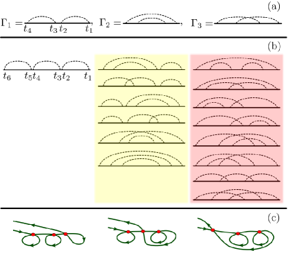
Figure 4: (Color online) (a) Three possible diagrams containing two dashed lines. Different pairings dictate the arguments of the diffusive propagators in the analytical expressions Eq. (I.2) for the diagrams. (b) Fifteen diagrams with three dashed lines arranged in three groups, white, yellow, and pink, according to their “complexity”. Different groups correspond to different mutual arrangements of the self-intersections in the underlying diffusive trajectories. Corresponding trajectories for the first diagrams of each group are sketched in (c).

The difference between the partial and actual sums can be estimated by considering the first neglected terms. Within the first variant of the partial summation we neglected $\frac{1}{2}\Gamma_{1}$, so that

$$\delta\langle S_{z}\rangle=\frac{b_{0}^{4}\tau t^{3}}{4\pi}\int\limits_{0}^{1}\!dx_{1}\int\limits_{0}^{x_{1}}\!\frac{dx_{2}}{\sqrt{x_{1}-x_{2}}}\int\limits_{0}^{x_{2}}\!dx_{3}\int\limits_{0}^{x_{3}}\!\frac{dx_{4}}{\sqrt{x_{3}-x_{4}}}.$$ (27)

The above integral can be evaluated analytically yielding

$$\delta\langle S_{z}\rangle=b_{0}^{4}\tau t^{3}\frac{\Gamma_{1}}{2}=\frac{1}{24}b_{0}^{4}\tau t^{3}.$$ (28)

In a similar fashion we can estimate the accuracy of the second partial sum in which the first neglected term is $\Gamma_{2}+\Gamma_{3}$. One has

$$\delta\langle S_{z}\rangle=\left(\frac{2}{9\pi}-\frac{1}{24}\right)b_{0}^{4}\tau t^{3}$$ (29)

Note that, while the two corrections Eq. (28) and Eq. (29) are almost equal in magnitude, the first one shifts the partial sum, $2\exp{\left[-\lambda_{1}(t)/2\right]}-1$, up, while the second one shifts the partial sum, $\exp{\left[-\lambda_{1}(t)\right]}$, down.

I.3 Self-consistent equation for $\langle S_{z}(t)\rangle$

Summation of the subset of diagrams with $n$ non-overlapping dashed arcs, Fig. 4, corresponds to retaining only the pairings $\phi(t_{1})=\phi(t_{2})$,  $\phi(t_{3})=\phi(t_{4})$, …. in Eq. (6). With these pairings, upon averaging of Eq. (6) over the hyperfine fields with the help of Eq. (8), the expression for the average $\langle S_{z}(t)\rangle$ assumes the form

$$\langle S_{z}(t)\rangle=\sum_{n=0}^{\infty}(-1)^{n}b_{0}^{2n}\mu^{(n)}(t),$$ (30)

where $\mu^{(n)}$ are the $2n$-fold integrals defined as

$$\mu^{(n)}(t)=\int\limits_{0}^{t}dt_{1}\int\limits_{0}^{t_{1}}dt_{2}C_{D}(t_{1},t_{2})\int\limits_{0}^{t_{2}}dt_{3}\int\limits_{0}^{t_{3}}dt_{4}C_{D}(t_{3},t_{4})....$$ (31)

It is apparent from Eq. (31) that these integrals satisfy the recurrence relation

$$\frac{d\mu^{(n+1)}}{dt}=\int\limits_{0}^{t}dt_{1}C_{D}(t,t_{1})\hskip 1.42262pt\mu^{(n)}(t_{1}).$$ (32)

Using this relation, the derivative $d\langle S_{z}\rangle/dt$ can be expressed via $\langle S_{z}\rangle$ as follows

$$\frac{d\langle S_{z}\rangle}{dt}=-\frac{b_{0}^{2}\tau^{1/2}}{(2\pi)^{1/2}}\int\limits_{0}^{t}\frac{dt^{\prime}}{\left(t-t^{\prime}\right)^{1/2}}\langle S_{z}(t^{\prime})\rangle,$$ (33)

where we have substituted the explicit form of the $1d$ diffusive correlator. Upon introducing a new variable $u=b_{0}^{2}\tau^{1/2}t^{3/2}$, Eq. (33) can be reduced to a dimensionless form

$$\frac{d\langle S_{z}\rangle}{du}=-\frac{4}{9(2\pi)^{1/2}u^{1/3}}\int_{0}^{u}\frac{du_{1}}{u_{1}^{1/3}\left(u^{2/3}-u_{1}^{2/3}\right)^{1/2}}\langle S_{z}(u_{1})\rangle.$$ (34)

Numerical solution of Eq. (34) exhibits rapidly decaying oscillations at $u\gg 1$. Only the first oscillation can be resolved in Fig. 3a. The depth of a corresponding minimum is $\langle S_{z}\rangle=-0.34$, i.e. it is approximately two times deeper than the minimum in the simulation result.

In the presence of $b_{z}$-component of the random hyperfine field $C_{D}(t_{1},t_{2})$ in Eq. (31) gets modified as

$$C_{D}(t_{1},t_{2})\rightarrow C_{D}(t_{1},t_{2})\left<\cos\left(-\int\limits_{t_{2}}^{t_{1}}b_{z}(s)ds\right)\right>.$$ (35)

Averaging of the cosine again reduces to the exponent

$$\left<\cos\left(-\int\limits_{t_{2}}^{t_{1}}b_{z}(s)ds\right)\right>=\exp\Bigl{[}-\frac{1}{2}\int\limits_{t_{1}}^{t_{2}}\int\limits_{t_{1}}^{t_{2}}dt^{\prime}dt^{\prime\prime}\langle b_{z}(t^{\prime})b_{z}(t^{\prime\prime})\rangle\Bigr{]}\\ =\exp\Bigl{[}-\frac{b_{0}^{2}}{4}\int\limits_{t_{1}}^{t_{2}}\int\limits_{t_{1}}^{t_{2}}dt^{\prime}dt^{\prime\prime}C_{D}(t^{\prime},t^{\prime\prime})\Bigr{]}.$$ (36)

Note that, unlike modification of a single dashed arc, the exponent contains diffusive correlator, $C_{D}(t^{\prime},t^{\prime\prime})$, rather than the short-time correlator $C_{0}(t^{\prime},t^{\prime\prime})$. With the above modification of $C_{D}(t_{1},t_{2})$, the self-consistent equation Eq. (33) takes the form

$$\frac{d\langle S_{z}\rangle}{dt}=-\frac{b_{0}^{2}\tau^{1/2}}{(2\pi)^{1/2}}\int\limits_{0}^{t}\frac{dt^{\prime}\exp\left[-b_{0}^{2}\tau^{1/2}(t-t^{\prime})^{3/2}\right]}{\left(t-t^{\prime}\right)^{1/2}}\langle S_{z}(t^{\prime})\rangle,$$ (37)

which leads to Eq. (18) of the main text.

References

(1) Z. H. Xiong, D. Wu, Z. V. Vardeny, and J. Shi, Nature
(London) 427, 821 (2004).
(2) S. Pramanik, C.-G. Stefanita, S. Patibandla, S. Bandyopadhyay, K. Garre, N. Harth, and M.
Cahay, Nat. Nanotechnol. 2, 216 (2007).
(3) V. A. Dediu, L. E. Hueso, I. Bergenti, and C. Taliani, Nat. Mater.8, 850 (2009).
(4) A. J. Drew, J. Hoppler, L. Schulz, F. L. Pratt, P. Desai, P. Shakya, T. Kreouzis, W. P. Gillin,
A. Suter, N. A. Morley, V. K. Malik, A. Dubroka, K. W. Kim, H. Bouyanfif, F. Bourqui, C.
Bernhard, R. Scheuermann, G. J. Nieuwenhuys, T. Prokscha, and E. Morenzoni, Nat. Mater. 8, 109
(2009).
(5) T. Nguyen, G. Hukic-Markosian, F. Wang, L. Wojcik, X. Li, E. Ehrenfreund, Z. Vardeny, Nat.
Mater. 9, 345 (2010).
(6) M. I. Dyakonov and V. I. Perel, Sov. Phys. Solid State 13,
3023 (1971).
(7) see Supplemental Material.
(8)
I. S. Lyubinskiy and V. Y. Kachorovskii, Phys. Rev. B 73, 041301 (2006).
(9) M. M. Glazov and E. Ya. Sherman, Europhys. Lett.
76, 102 (2006).
(10) C. Echeverria-Arrondo and E. Ya. Sherman, Phys. Rev. B 85, 085430 (2012).
(11) R. C. Roundy and M. E. Raikh, Phys. Rev. B 88, 205206 (2013).
(12) R. C. Roundy, D. Nemirovsky, V. Kagalovsky, and M. E. Raikh,
arXiv:1311.0338.
(13) B. L. Altshuler, D. Khmel’nitzkii, A. I. Larkin, and P. A. Lee, Phys. Rev. B 22, 5142 (1980).