Numerical Study of the semiclassical limit of the Davey-Stewartson II equations

Abstract

We present the first detailed numerical study of the semiclassical limit of the Davey-Stewartson II equations both for the focusing and the defocusing variant. We concentrate on rapidly decreasing initial data with a single hump. The formal limit of these equations for vanishing semiclassical parameter $\epsilon$, the semiclassical equations, are numerically integrated up to the formation of a shock. The use of parallelized algorithms allows to determine the critical time $t_{c}$ and the critical solution for these $2+1$-dimensional shocks. It is shown that the solutions generically break in isolated points similarly to the case of the $1+1$-dimensional cubic nonlinear Schrödinger equation, i.e., cubic singularities in the defocusing case and square root singularities in the focusing case. For small values of $\epsilon$, the full Davey-Stewartson II equations are integrated for the same initial data up to the critical time $t_{c}$. The scaling in $\epsilon$ of the difference between these solutions is found to be the same as in the $1+1$ dimensional case, proportional to $\epsilon^{2/7}$ for the defocusing case and proportional to $\epsilon^{2/5}$ in the focusing case.

We document the Davey-Stewartson II solutions for small $\epsilon$ for times much larger than the critical time $t_{c}$. It is shown that zones of rapid modulated oscillations are formed near the shocks of the solutions to the semiclassical equations. For smaller $\epsilon$, the oscillatory zones become smaller and more sharply delimited to lens shaped regions. Rapid oscillations are also found in the focusing case for initial data where the singularities of the solution to the semiclassical equations do not coincide. If these singularities do coincide, which happens when the initial data are symmetric with respect to an interchange of the spatial coordinates, no such zone is observed. Instead the initial hump develops into a blow-up of the $L_{\infty}$ norm of the solution. We study the dependence of the blow-up time on the semiclassical parameter $\epsilon$.

1 Introduction

Nonlinear Schrödinger (NLS) equations have many applications, e.g. in hydrodynamics, plasma physics and nonlinear optics where they can be used to model the amplitude modulation of weakly nonlinear, strongly dispersive waves. They can be cast into the form

$$i\epsilon\Psi_{t}+\frac{\epsilon^{2}}{2}\Delta\Psi-\frac{\rho}{\sigma}\left|\Psi\right|^{2\sigma}\Psi=0,\,\,x\in\mathbb{R}^{d}\,\,,t\in\mathbb{R},$$ (1)

where $\Psi$ is a complex valued function, $\Delta$ is the Laplace operator in $d$ dimensions, and $\epsilon\ll 1$ is a real positive parameter. The exponent $1<2\sigma<\infty$ represents the power of the nonlinearity, and the parameter $\rho=\pm 1$ determines whether this nonlinearity has a focusing ($\rho=-1$) or a defocusing ($\rho=1$) effect. The cubic (i.e., $\sigma=1$) $1+1$-dimensional NLS is known to be completely integrable [64] which implies that many exact solutions as solitons and breathers can be given in explicit form.

Since the parameter $\epsilon$ in (1) has the same role as the Planck constant $\hbar$ in the classical Schrödinger equation in quantum mechanics, the limit $\epsilon\to 0$ is also referred to as the semiclassical limit. This limit is mathematically challenging since it complements the well known difficulties of the semiclassical limit in quantum mechanics (highly oscillatory functions) with the nonlinearity of the NLS equation (1), which typically leads to strong gradients. Note that the parameter $\epsilon$ can be introduced into the dimensionless form of the NLS equation (eq. (1) with $\epsilon=1$) via a rescaling of the coordinates of the form $x\to x/\epsilon$, and $t\to t/\epsilon$. Thus the introduction of a small $\epsilon$ can be seen as equivalent to studying the solution of a Cauchy problem for initial data with support on scales of order $1/\epsilon$ for long times of order $1/\epsilon$. With the well known Wenzel-Kramer-Brillouin (WKB) ansatz, also known as Madelung transform [41] in this context,

$$\Psi=\sqrt{u}e^{iS/\epsilon},$$ (2)

for $u$ and $S$ being real valued functions, the initial value problem $\Psi(x,0)=\Psi_{0}(x)$ for the NLS equation (1) is equivalent to

$$\left\{\begin{array}[]{ccc}u_{t}+\mbox{div}(u\cdot w)&=&0\\ w_{t}+w\cdot\nabla w+\rho\nabla u^{2\sigma}&=&\frac{\epsilon^{2}}{2}\nabla\left(\frac{\Delta(\sqrt{u})}{\sqrt{u}}\right),\\ u(x,0)=u_{0}(x),\,\,w(x,0)=w_{0}(x)\end{array}\right.$$ (3)

where $w=\nabla S$. This form of the NLS equation is also referred to as the hydrodynamic form due to its similarity with the compressible Euler equation which are obtained in the formal limit $\epsilon=0$,

$$\left\{\begin{array}[]{ccc}u_{t}+\mbox{div}(u\cdot w)&=&0\\ w_{t}+w\cdot\nabla w+\rho\nabla u^{2\sigma}&=&0\\ u(x,0)=u_{0}(x),\,\,w(x,0)=w_{0}(x)\end{array}\right.$$ (4)

and that we call the semiclassical NLS system in the following.

In the defocusing $1+1$-dimensional case ($\rho=1$), this system is hyperbolic, and the corresponding initial value problem is well-posed. It describes an isentropic gas which can develop a gradient catastrophe in finite time similar to the shock formation in solutions to the Hopf equation $u_{t}+uu_{x}=0$. The generic behavior of the solutions at the critical points is given by a cubic singularity. The defocusing NLS equation for finite small $\epsilon$ can be seen as a dispersive regularization of the system (4). Its solutions have rapid modulated oscillations in the vicinity of the gradient catastrophe of solutions of the system (4) for the same initial data called dispersive shocks. Using the complete integrability, Jin, Levermore and McLaughlin [28] gave an asymptotic description of the oscillatory zone in solutions to the defocusing cubic NLS. The situation is very similar to the Korteweg-de Vries equation (KdV) for which a complete asymptotic theory of dispersive shocks was developed in [39, 63, 14]. A first numerical implementation of the asymptotic description for KdV was presented in [25]. No such theory exists for non-integrable cases. Before the critical time $t_{c}$ of the semiclassical solution and in the exterior of the oscillatory zone, the solution of the system (4) for the same initial data gives an asymptotic description of the NLS solution for $\epsilon\to 0$. The behavior for $t\sim t_{c}$ has been addressed in [19] for a large class of two-component systems including $1+1$-dimensional NLS equations, also for non-integrable cases. It is conjectured that the solution near $t_{c}$ to such equations is given in order $\epsilon^{2/7}$ by a rescaled unique solution to an ordinary differential equation (ODE), the second equation in the Painlevé I hierarchy (PI2). The conjecture in [19] essentially states that the formation of a dispersive shock close to $t_{c}$ is equivalent to the corresponding situation in KdV solutions for which Dubrovin presented a conjecture in [17] for a large class of scalar equations containing KdV. The conjecture was proven for KdV with Riemann-Hilbert techniques by Claeys and Grava in [13]. The existence of the conjectured PI2 solution regular on the whole real line was proven in [60]. Note that the conjecture in [19] postulates a universality property of hyperbolic dispersive shocks in the sense that the solutions near the break-up of the dispersionless or semiclassical limit are asymptotically given in terms of the PI2 transcendent for a large class of dispersive partial differential equations (PDEs) and a large class of initial data.

The situation in the $1+1$-dimensional focusing case ($\rho=-1$) is more involved since the system (3) is elliptic which implies an ill-posed Cauchy problem. The generic singularities forming in solutions to (4) for analytic initial data are of elliptic umbilic type as was shown in [18]. In the semiclassical limit, zones of rapid modulated oscillations again form near such a singularity. In contrast to the defocusing NLS equation, an asymptotic description of the oscillatory zone has been given only for certain classes of initial data in [27, 29, 61]. The behavior close to the critical time $t_{c}$ of the semiclassical system (4) was addressed in [18] for the integrable cubic case, and has been recently generalized to a large class of two-component systems including generalized NLS equations in [19]. It is conjectured that the NLS solution for $t\sim t_{c}$ is given by a rescaled tritronquée solution [8] of the Painlevé I equation in order $\epsilon^{2/5}$. A partial proof of this conjecture for the integrable cubic case was given in [40].

The questions discussed above for the $1+1$-dimensional case are mostly wide open for $2+1$-dimensional settings. First numerical attempts in this direction were presented in [35, 33, 52]. In [34] a detailed numerical study of the formation of dispersive shocks in the Kadomtsev-Petviashvili (KP) equation (a $2+1$-dimensional generalization of KdV) was given. Here we present a numerical study of the semiclassical limit of NLS equations in $2+1$ dimensions. Since the strongest results in the asymptotic description of $1+1$-dimensional PDEs have been obtained with techniques from the theory of integrable systems, we concentrate here on an integrable nonlocal NLS equation in $2+1$ dimensions, the Davey-Stewartson (DS) system,

$$\begin{array}[]{ccc}i\epsilon\Psi_{t}+\epsilon^{2}\left(\Psi_{xx}-\alpha\Psi_{yy}\right)+2\rho\left(\Phi+\left|\Psi\right|^{2}\right)\Psi&=&0,\\ \Phi_{xx}+\beta\Phi_{yy}+2\left|\Psi\right|_{xx}^{2}&=&0,\end{array}$$ (5)

where $\alpha,\beta$ and $\rho$ take the values $\pm 1$, $\epsilon\ll 1$ is a small dispersion parameter, and $\Phi$ is a mean field. These systems describe the amplitude modulation of weakly nonlinear, strongly dispersive $2+1$-dimensional waves in hydrodynamics and nonlinear optics, and appear also in plasma physics to describe the evolution of a plasma under the action of a magnetic field. They have been classified in [24] as elliptic-elliptic, hyperbolic-elliptic, elliptic-hyperbolic and hyperbolic-hyperbolic, according to the signs of $\alpha$ and $\beta$. The DS system is known to be completely integrable when $\alpha=\beta$ [1]. The case $\alpha=\beta=-1$ is also called DS I, the case $\alpha=\beta=1$, DS II. We concentrate here on the latter where the mean field $\Phi$ is governed by an elliptic equation which can be solved uniquely with some fall off condition at infinity. Then $\Phi=\mathcal{M}\left(|\Psi|^{2}\right)$, where the operator $\mathcal{M}$ is defined in Fourier space by

$$\widehat{\mathcal{M}(f)}=\frac{-2k_{x}^{2}}{k_{x}^{2}+k_{y}^{2}}\widehat{f}(k_{x},k_{y}),$$

where $k_{x}$ and $k_{y}$ represent the wave numbers, in the $x$ and $y$ directions, respectively, and where $\hat{f}$ denotes the Fourier transform of a function $f$. With the operators $\mathcal{D}_{\pm}=\partial_{x}^{2}\pm\partial_{y}^{2}$, the DS II equations can be written in the form

$$i\epsilon\Psi_{t}+\epsilon^{2}\mathcal{D}_{-}\Psi-2\rho(\mathcal{D}_{+}^{-1}\mathcal{D}_{-}|\Psi|^{2})\Psi=0,$$ (6)

where $\mathcal{D}_{+}^{-1}$ is defined as above by its Fourier symbol. Thus DS II can be seen as an NLS equation with a nonlocal (due to the operator $\mathcal{D}_{+}^{-1}$) cubic nonlinearity. Similarly to the NLS equation, the latter admits a focusing ($\rho=-1$) and a defocusing $\rho=1$ version.

Note, however, that the operator $\mathcal{D}_{-}$ leads to a different dynamics compared to the standard NLS equation (1) with a Laplace operator. Therefore many PDE techniques successful for NLS could not be applied to the DS II equation. Using integrability, Fokas and Sung [6, 59] studied the existence and long-time behavior of the solutions of the initial value problem for DS II (for $\epsilon=1$, and $\Psi(x,y,0)=\Psi_{0}$). They proved the following

Theorem 1.

If $\Psi_{0}$ belongs to the Schwartz space $\mathcal{S}(\mathbb{R}^{2})$, then there exists in the defocusing case ($\rho=1$) a unique global solution $\Psi$ to DS II such that $t\mapsto\Psi(\cdot,t)$ is a $C^{\infty}$ map from $\mathbb{R}\mapsto\mathcal{S}(\mathbb{R}^{2})$. The same holds for the focusing case ($\rho=-1$) if the initial data $\Psi_{0}\in L_{q}$ for some $q$ with $1\leq q<2$ have a Fourier transform $\widehat{\Psi_{0}}\in L_{1}\cap L_{\infty}$ such that $\|\widehat{\Psi_{0}}\|_{L_{1}}\|\widehat{\Psi_{0}}\|_{L_{\infty}}<\frac{\pi^{3}}{2}\left(\frac{\sqrt{5}-1}{2}\right)^{2}$. The unique global solution $\Psi$ to DS II satisfies the decay estimate $\|\Psi(t)\|_{L_{\infty}}<\frac{const}{t}$.
Furthermore, if $\Psi_{0}$ belongs to the Schwartz space $\mathcal{S}(\mathbb{R}^{2})$, then there is an infinite number of conserved quantities.

The first in a hierarchy of conserved quantities are the wave energy $N:=\int_{\mathbb{R}^{2}}|\Psi(x,y,t)|^{2}dxdy$, the linear momentum $P:=\int_{\mathbb{R}^{2}}i\left(\Psi^{\ast}\nabla\Psi-\Psi\nabla\Psi^{\ast}\right)dxdy$, and the energy

$$E :=\frac{1}{2}\int_{\mathbb{R}^{2}}\bigg{[}\epsilon^{2}|\Psi_{x}|^{2}-\epsilon^{2}|\Psi_{y}|^{2}-\rho\left(|\Psi|^{4}-\frac{1}{2}\left(\Phi^{2}+(\partial_{x}^{-1}\Phi_{y})^{2}\right)\right)\bigg{]}dxdy.$$ (7)

The smallness condition in Theorem 1 indicates that there might be a blow-up, i.e., a loss of regularity with respect to the initial data, in solutions to the focusing DS II equations. In fact, for focusing cubic NLS equations, $2+1$ dimensions constitute the critical dimension where blow-up can occur. However due to the operator $\mathcal{D}_{-}$ in (6) this cannot be directly generalized to DS II. Therefore it is important in this context that Ozawa gave an exact blow-up solution in [49]. The solution is similar to the well known lump solutions [4], travelling solitonic wave solutions with an algebraic fall off at infinity. Note that Theorem 1.1 does not hold for lumps since they are not in $L_{1}(\mathbb{R}^{2}$). It is thus not known whether there is generic blow-up for initial data not satisfying this condition, nor whether the condition is optimal. Numerical studies in [46, 32] indicate, however, that blow-up can occur in perturbations of the lump and the Ozawa solution and is thus a generic feature of solution to the focusing DS II. In fact it was conjectured in [46] that generic localized initial data are either just radiated away to infinity or blow up for large $t$.

Therefore it is not obvious whether dispersive shocks can be observed at all in focusing DS II systems, or whether the solutions blow-up directly. Numerically it was shown in [33, 52] that dispersive shocks can indeed be seen. In the semiclassical limit ($\Psi=\sqrt{u}e^{iS/\epsilon},\,\,\epsilon\to 0$), DS II reduces to the following system

$$\left\{\begin{array}[]{ccc}S_{t}+S^{2}_{x}-S^{2}_{y}+2\rho\mathcal{D}_{+}^{-1}\mathcal{D}_{-}(u)&=&\frac{\epsilon^{2}}{2}\left(\frac{u_{x}x}{u}-\frac{u_{x}^{2}}{u^{2}}-\frac{u_{y}y}{u}+\frac{u_{y}^{2}}{u}\right)\\ u_{t}+2\left(S_{x}u\right)_{x}-2\left(S_{y}u\right)_{y}&=&0\\ \end{array}\right.,$$ (8)

with the formal limit $\epsilon\to 0$

$$\left\{\begin{array}[]{ccc}S_{t}+S^{2}_{x}-S^{2}_{y}+2\rho\mathcal{D}_{+}^{-1}\mathcal{D}_{-}(u)&=&0\\ u_{t}+2\left(S_{x}u\right)_{x}-2\left(S_{y}u\right)_{y}&=&0\\ \end{array}\right.,$$ (9)

which will be referred to as the semiclassical DS II system in the following. This system is not integrable in the usual sense that it can be associated to a standard Riemann-Hilbert problem (RHP), but it is integrable in the sense of hydrodynamic reductions [36]. It is an open question whether it can be treated with the nonlinear RHP approach proposed in [42, 43, 44] for dispersionless $2+1$-dimensional PDEs as the dispersionless KP (dKP) or the two-dimensional Toda equation in the long wavelength limit. It is also not clear whether it can be treated via infinite Frobenius manifolds as in [23, 51] for these two PDEs.

Therefore we will present in this paper the first comprehensive numerical study of the semiclassical limit of DS II equations. This is a highly nontrivial task already in $1+1$ dimensions, and will be even more so with an additional spatial dimension. To obtain the necessary resolution, we will use parallel computing. Firstly we have to integrate the semiclassical DS II system up to a break-up of the solution, i.e, up to the formation of a singularity of the solution which is numerically extremely challenging. Since we want to study various scalings in $\epsilon$ for DS II solutions close to the critical time $t_{c}$, the latter has to be reliably identified. A careful numerical investigation in [34] for the dKP equation allowed to study the small dispersion limit of KP solutions close to the break-up of the corresponding dKP solution. In particular, it could be shown that the difference between the KP and dKP solutions for the same initial data shows the same characteristic scaling in $\epsilon$ as the one-dimensional model (KdV/Hopf). The main technique used was asymptotic Fourier analysis as first applied numerically in [57] to trace singularities in the complex plane. In this framework the singularity of the real solution appears when one of the singularities in the complex plane hits the real axis. This method will also allow here to identify both the critical time $t_{c}$ of solutions to the semiclassical DS II system (9) and the critical solution. We obtain the following

Conjecture 2.

Consider rapidly decreasing smooth initial data in $L_{2}(\mathbb{R}^{2})$ with a single maximum. Then

• Solutions to the defocusing variant of the semiclassical DS II equation (9) show the same type of break-up as for the corresponding limit of the $1+1$-dimensional NLS equation: the solutions have two break-up points in each spatial direction (not necessarily on the coordinate axes and at the same time) which are generically of cubic type as for generic solutions to the Hopf equation.

• Solutions of the focusing variant of the semiclassical DS II equation (9) have in general two break-up points of the same type as solutions of the focusing $1+1$-dimensional NLS equation, a square root cusp for each spatial direction. For initial data with a symmetry with respect to an interchange of the spatial coordinates, these cusps appear at the same time and location.

Secondly, the DS II equation is a purely dispersive equation. For such equations, the introduction of numerical dissipation has to be limited as much as possible, to avoid the suppression of dispersive effects. Therefore we use Fourier spectral methods for the spatial dependence of the solution as well. In addition, focusing NLS and DS equations are known to have a modulational instability, i.e., self-induced amplitude modulation of a continuous wave propagating in a nonlinear medium, which has dramatic consequences in numerics, see e.g. [31], if not sufficient spatial resolution is used. Moreover an efficient time integrator of high accuracy is needed in order not to pollute the Fourier coefficients. As will be shown in the paper, the applied methods allow to solve the DS II equation and to identify the scaling in $\epsilon$ of the difference between DS II (8) and semiclassical DS II (9) solution at the critical time. The main results of the study for rapidly decreasing (in both spatial directions) initial data with a single hump for the DS II equations can be summarized in the following

Conjecture 3.

Consider rapidly decreasing smooth initial data in $L_{2}(\mathbb{R}^{2})$ with a single maximum. Then

• The difference of solutions to the defocusing semiclassical DS II equation (9) at the critical time $t_{c}$ and the solutions to the defocusing DS II equation for the same initial data and different values of $\epsilon$ scales as $\epsilon^{2/7}$ as in the case of the $1+1$-dimensional defocusing NLS equation.

• The difference of solutions to the focusing semiclassical DS II equation (9) at the critical time $t_{c}$ and the solutions to the focusing DS II equation for the same initial data and different values of $\epsilon$ scales as $\epsilon^{2/5}$ as in the case of the $1+1$-dimensional focusing NLS equation.

• For times $t\gg t_{c}$, solutions to the defocusing DS II equation show for small $\epsilon$ zones of rapid modulated oscillations in the vicinity of the critical points of the solutions of (9) for the same initial data.

• For times $t\gg t_{c}$ and initial data where the two cusps do not appear at the same time and location, solutions to the focusing DS II equation show for small $\epsilon$ zones of rapid modulated oscillations: the initial hump breaks up for $t>t_{c}$ into an array of smaller humps forming a cusped zone in the $x,y,t$ space.

• For the focusing DS II equation, initial data with a symmetry with respect to an interchange of $x$ and $y$ lead to a blow-up of the $L_{\infty}$ norm of the solution in finite time $t^{*}$ for sufficiently small $\epsilon$. There is no oscillatory zone for $|\Psi|^{2}$ in this case, the initial hump evolves directly into a singularity. The difference between blow-up time $t^{*}$ and break-up time $t_{c}$ scales roughly as, $t^{*}-t_{c}\propto\epsilon$. The blow-up time is always larger than the break-up time.

The paper is organized as follows: in section 2, we describe the various numerical methods used. In section 3, we illustrate the use of asymptotic Fourier analysis for the semiclassical $1+1$-dimensional NLS system, for which explicit results are known. Then we apply these methods to the semiclassical DS II system (9). In section 4, we study the behavior of the solutions of DS II for small $\epsilon$, and establish scaling laws in $\epsilon$ for the difference between semiclassical DS II and DS II solution at break-up. In section 5 we investigate blow-up in DS II solutions for small $\epsilon$. We add some concluding remarks in section 6.

2 Numerical Methods

In this section we summarize the numerical approaches used in this paper. The task is to study numerically two different kinds of systems, the first one being a coupled system of nonlinear dispersionless equations (9), the second one being a nonlinear dispersive PDE of NLS type (6). For both, we will consider a periodic setting for the spatial coordinates, which allows the use of a Fourier spectral method for the space discretization. We treat the rapidly decreasing functions we are studying as essentially periodic analytic functions within the finite numerical precision. For such functions, spectral methods are known for their excellent (in practice exponential) approximation properties, see for instance [10, 62]. In addition they introduce only very little numerical dissipation which is important in the study of dispersive effects. Last but not least we use the Fourier coefficients of the solutions to the semiclassical systems to identify the break-up of the solution as in [57, 34].

In all cases, the numerical precision is controlled via the numerically computed energy for each system considered. More precisely, given $E$, a conserved quantity of the system, the numerically computed $E$ will depend on time due to unavoidable numerical errors. It was shown for instance in [31, 33] that the conservation of $E$ in the form of the quantity

$$\Delta_{E}=\left|\frac{E(t)}{E(0)}-1\right|$$ (10)

can be used as a reliable indicator of numerical accuracy, provided that there is sufficient spatial resolution (generally the accuracy of the numerical solution is overestimated by two orders of magnitude). We always aim at a $\Delta_{E}$ smaller than $10^{-6}$ to ensure an accuracy well beyond the plotting accuracy $\sim 10^{-3}$.

2.1 Dispersionless Systems

The most difficult task in the solution of the dispersionless systems is to identify numerically the break-up of the solution with sufficient accuracy to allow the scaling studies we are interested in. To this end we have to compute the solution up to the time of gradient catastrophe, and both this time and the solution should be found with sufficient accuracy. To do so, we will use asymptotic Fourier analysis as first applied numerically by Sulem, Sulem and Frisch in [57]. The basic idea of this method is that functions analytic in a strip around the real axis in the complex plane have a characteristic Fourier spectrum for large wave numbers. Thus it is in principle possible to obtain the width of the analyticity strip from the asymptotic behavior of the Fourier transform of the solution (in one spatial dimension), or from the angle averaged energy spectrum in higher dimensions. This allows in particular to identify the time when a singularity in the complex plane hits the real axis and thus leads to a singularity of the function on the real line. Singular solutions to the two-dimensional cubic NLS equation have been studied with this approach in [58], and an application of the method to the two-dimensional Euler equations can be found in [22, 45]. The method has also been applied to the study of complex singularities of the three-dimensional Euler equations in [9], in thin jets with surface tension [50], the complex Burgers’ equation [54] and the Camassa-Holm equation [15]. More recently, we investigated its efficiency quantitatively for the Hopf equation and showed that the method can be efficiently used in practice to describe the critical behavior of solutions to dispersionless equations. As an example, a study of the break up of dKP solutions for certain classes of initial data has been presented in [34]. If $u(z)$ is an analytic function of one variable $z\in\mathbb{C}$ such that $|u(z)|\to 0$ uniformly as $|z|\to\infty$, and if the singularities of $u(z)$ are isolated and of the form $u\sim(z-z_{j})^{\mu_{j}}$, $\mu_{j}\notin\mathbb{Z}$, with $z_{j}=\alpha_{j}-i\delta_{j}$, $\alpha_{j},\delta_{j}\in\mathbb{R}$ in the lower half plane ($\delta_{j}\geq 0$), a steepest descent argument for $k\to\infty$ implies the following asymptotic behavior of the Fourier coefficients (for a detailed derivation see e.g. [11]),

$$\hat{u}\sim\sqrt{2\pi}\mu_{j}^{\mu_{j}+\frac{1}{2}}e^{-\mu_{j}}\frac{(-i)^{\mu_{j}+1}}{k^{\mu_{j}+1}}e^{-ik\alpha_{j}-k\delta_{j}},$$ (11)

where $\hat{u}$ is the Fourier transform of $u(x)\in L^{2}(\mathbb{R})$, defined as

$$\hat{u}(k)=\int_{\mathbb{R}}u(x)e^{-ikx}dx.$$ (12)

Consequently for a single such singularity with positive $\delta_{j}$, the modulus of the Fourier coefficients decreases exponentially for large $k$. For $\delta_{j}=0$, i.e., a singularity on the real axis, the modulus of the Fourier coefficients has an algebraic dependence on $k$, and thus the location of singularities in the complex plane can be obtained from a given Fourier series computed on the real axis. If there are several singularities of this form at $z_{j}$, $j=1,\ldots,J$, there will be oscillations in the modulus of the Fourier coefficients for moderately large $k$.

To numerically compute a Fourier transform, it has to be approximated by a discrete Fourier series which can be done efficiently via a fast Fourier transform (FFT), see e.g. [62]. The discrete Fourier transform of the vector $\mathbf{u}$ with components $u_{j}=u(x_{j})$, where $x_{j}=2\pi Lj/N$, $j=1,\ldots,N$ (i.e., the Fourier transform on the interval $[0,2\pi L]$ where $L$ is a positive real number) will be always denoted by $v$ in the following. There is no obvious analogue of relation (11) for a discrete Fourier series, but it can be seen as an approximation of the former, which is also the basis of the numerical approach in the solution of the PDE. It is possible to establish bounds for the discrete series, see for instance [5].

According to (11), $v$ is assumed to be of the form $v(k,t)\underset{k\to\infty}{\sim}e^{A(t)}k^{-B(t)}e^{-\delta(t)k},$ and one can trace the temporal behavior of $\delta(t)$ obtained via some fitting procedure in order to obtain evidence for the formation of a singularity on the real line (the problem is reduced to check if $\delta(t)$ vanishes at a finite time $t_{c}$). In order to determine $\delta(t)$ from direct numerical simulations, a least-square fit is performed on the logarithm of the Fourier transform in the form

$$\ln|v|\sim A-B\ln k-k\delta.$$ (13)

The fitting is done for a given range of wave numbers $k_{min}<k<k_{max}$ (we only consider positive $k$), that have to be controlled, as explained in detail in [34]. The critical time $t_{c}$ is determined by the vanishing of $\delta$, and the type of the singularity is given by the parameter $B(t_{c})$ which is equal to $\mu_{j}+1$. One can also determine the real part of the location of the singularity by doing a least square fitting on the imaginary part of the logarithm of $v$ for which one has asymptotically

$$\phi:=\Im\ln v\sim C-\alpha k.$$ (14)

Since the logarithm is branched in Matlab/Fortran at the negative real axis with jumps of $2\pi$, the computed $\phi$ will in general have many jumps. Thus one has first to construct a continuous function from the computed $\phi$, as explained in [34]. Then the location of the singularity on the real axis is given by $\alpha(t_{c})$.

Obviously the choice of the fitting bounds $(k_{min},k_{max})$ has an impact on the determination of the fitting parameters, and we carefully investigated this issue in [34]. There we found that in order to obtain reliable results, high space resolution has to be used (typically $2^{14}$ or more Fourier modes in each space directions). This implies in particular that for the study of 2+1-dimensional problems, codes have to be parallelized, see below. Moreover, a procedure to obtain the ‘minimal error fitting bounds’ whilst using at least half of the Fourier coefficients has been proposed. Obviously, only the values for which the Fourier coefficients have a greater modulus than the numerical error have to be considered (we choose this threshold to be $|v|>10^{-10}$). Now, let $f_{e}$ denote a prescribed value for $\Delta=\|\ln|v|-(A-B\ln k-k\delta)\|_{\infty}$ referred to as fitting error in the following. Then, one can determine the minimal fitting error $\min(f_{e})$ that can be reached, by using at least half of the Fourier coefficients available for the studied problem, by choosing a suitable lower threshold (which depends on the problem), and by varying the upper limit to reach $f_{e}$.

Remark 4.

The minimal distance in Fourier space is $m:=2\pi L/N$ with $N$ being the number of Fourier modes and $2\pi L$ the length of the computational domain in physical space. Thus this defines the smallest distance which can be resolved in Fourier space. All values of $\delta$ below this threshold cannot be distinguished numerically from 0.

In [34], the identification of the break-up in dKP solutions could be done by studying only the Fourier transform as in (11) in one dimension, since only a one-dimensional break-up was conjectured to occur. Here a true two-dimensional singularity is possible, and instead of the Fourier transform $\hat{u}(k,t)$, one can consider as in [58] the angle averaged energy spectrum defined by

$$\mathcal{E}(K,t)=\underset{K<|k^{\prime}|<K+1}{\sum}|\hat{u}(k^{\prime},t)|^{2},$$ (15)

where $|k^{\prime}|=\sqrt{k_{x}^{2}+k_{y}^{2}}$. Slightly weaker estimates hold for $\mathcal{E}(K,t)$ for an analytic function $u$ and thus, to apply the asymptotic fitting to the Fourier coefficients, one assumes that $\mathcal{E}(K,t)=e^{A(t)}K^{-\alpha(t)}e^{-\delta(t)K},$ and performs the fitting on

$$\ln|\mathcal{E}|\sim A_{2d}-B_{2d}\ln K-K\delta_{2d}.$$ (16)

Similarly to the one-dimensional case, the appearance of a real singularity implies that $\delta(t)$ vanishes at a finite time $t_{c}$, and the descriptions given above hold except for the determination of $\alpha$.

For the numerical integration of the semiclassical DS II system (9), we thus use a Fourier discretization which leads to a large system of ODEs. In principle any ODE solver can be applied for the time integration. Typically we use the explicit fourth order Runge-Kutta scheme (RK4), and study the asymptotic behavior of the Fourier coefficients as explained above. We also use a Krasny filter [37] with a prescribed error of $10^{-14}$, which means that Fourier coefficients with a modulus of $10^{-14}$ and smaller are put equal to 0. This allows to reduce computer roundoff errors and to perform accurate computations with a larger number of points.

2.2 Dispersive PDEs

The situation is more involved for the study of dispersive PDEs. We again use a Fourier discretization for the spatial coordinates for the reasons explained above. Approximating the spatial dependence via truncated Fourier series leads for the studied equations (1) and (6) to large stiff systems of ODEs in Fourier space of the form

$$v_{t}=\mathbf{L}v+\mathbf{N}(v,t),$$ (17)

where $v$ is again the discrete Fourier transform of $\Psi$, and where $\mathbf{L}$ and $\mathbf{N}$ denote linear and nonlinear operators, respectively. These systems of ODEs are classical examples of stiff equations where the stiffness is related to the linear part $\mathbf{L}$ (it is a consequence of the distribution of the eigenvalues of $\mathbf{L}$), whereas the nonlinear part contains only low order derivatives.

There are several approaches to deal efficiently with equations of the form (17) with a linear stiff part as implicit-explicit (IMEX), time splitting, integrating factor (IF) as well as sliders and exponential time differencing. By performing a comparison of stiff integrators for the 1+1-dimensional cubic NLS equation in the semiclassical limit (1) in [31], and for the semiclassical limit of the DS II equation in [33], it was shown that Driscoll’s composite Runge-Kutta (DCRK) method [16] is very efficient in this context. We thus use this scheme for the time integration here.

The basic idea of the DCRK method is inspired by IMEX methods, i.e., the use of a stable implicit method for the linear part of the equation (17), which introduces the stiffness into the system, and an explicit scheme for the nonlinear part which is assumed to be non-stiff. Classic IMEX schemes do not perform in general satisfactorily for dispersive PDEs [30]. Driscoll’s [16] more sophisticated variant consists in splitting the linear part of the equation in Fourier space into regimes of high and low frequencies, and to use the fourth order RK integrator for the low frequencies and the nonlinear part, and the linearly implicit RK method of order three for the high frequencies. He showed that this method is in practice of fourth order over a wide range of step sizes.

An additional problem here is the modulational instability of the focusing NLS equations, i.e., a self-induced amplitude modulation of a continuous wave propagating in a nonlinear medium, with subsequent generation of localized structures, see for instance [2, 12, 20] for the NLS equation. This instability leads to an artificial increase of the high wave numbers which eventually breaks the code, if not enough spatial resolution is provided (see for instance [31] for the focusing NLS equation). It is not possible to reach the necessary resolution on single processors which makes a parallelization of the codes obligatory.

2.3 Parallelization for 2+1-dimensional problems

To be able to provide the high space resolution needed for the DS II simulations (see above), the numerical codes for the 2+1-dimensional problems have been parallelized. This can be conveniently done for two-dimensional Fourier transforms where the task of the one-dimensional FFTs is performed simultaneously by several processors. This reduces also the memory requirements per processor with respect to alternative approaches such as finite difference or finite element methods. We consider periodic (up to numerical precision) solutions in $x$ and $y$, i.e., solutions on $\mathbb{T}^{2}\times\mathbb{R}$. The computations are carried out with $N_{x}\times N_{y}$ points for $(x,y)\in[-L_{x}\pi,L_{x}\pi]\times[-L_{y}\pi,L_{y}\pi]$. In the computations, $L_{x}=L_{y}$ is chosen large enough such that the numerical solution is of the order of machine precision ($\sim 10^{-16}$ here) at the boundaries.

A prerequisite for parallel numerical algorithms is that sufficient independent computations can be identified for each processor, that require only small amounts of data to be communicated between independent computations. To this end, we perform a data decomposition, which makes it possible to do basic operations on each object in the data domain (vector, matrix…) to be executed safely in parallel by the available processors. Our domain decomposition is implemented by developing a code describing the local computations and local data structures for a single process. Global arrays are divided in the following way: denoting by $x_{n}=2\pi nL_{x}/N_{x},\,\,y_{m}=2\pi mL_{y}/N_{y}$, $n=-N_{x}/2,...,N_{x}/2,\,\,m=-N_{y}/2,...,N_{y}/2,$ the respective discretizations of $x$ and $y$ in the corresponding computational domain, $u$ (respectively $\Psi$) is then represented by a $N_{x}\times N_{y}$ matrix. For programming ease and for the efficiency of the Fourier transform, $N_{x}$ and $N_{y}$ are chosen to be powers of two. The number $n_{p}$ of processes is chosen to divide $N_{x}$ and $N_{y}$ perfectly, so that each processor $P_{i},i=1...n_{p}$, will receive $N_{x}\times\frac{N_{y}}{n_{p}}$ elements of $u$ corresponding to the elements

$$u\left(1:N_{x},(i-1).\frac{N_{y}}{n_{p}}+1:i.\frac{N_{y}}{n_{p}}\right)$$ (18)

in the global array, and then each parallel task works on a portion of the data.

While processors execute an operation, they may need values from other processors. The above domain decomposition has been chosen such that the distribution of operations is balanced and that the communication is minimized. The access to remote elements has been implemented via explicit communications, using sub-routines of the MPI (Message Passing Interface) library [26].

Actually, the only part of our codes that requires communications is the computation of the two-dimensional FFT and the fitting procedure for the Fourier coefficients. For the former we use the transposition approach. The latter allows to use highly optimized single processor one-dimensional FFT routines, that are normally found in most architectures, and a transposition algorithm can be easily ported to different distributed memory architectures. We use the well known FFTW library because its implementation is close to optimal for serial FFT computation, see [21]. Roughly speaking, a two-dimensional FFT does one-dimensional FFTs on all rows and then on all columns of the initial global array. We thus first transform in $x$ direction, each processor transforms all the dimensions of the data that are completely local to it, and the array is transposed once this has been done by all processors. Since the data are evenly distributed among the MPI processes, this transpose is efficiently implemented using MPI ALLTOALL communications of the MPI library.

The asymptotic fitting of the Fourier coefficients in one spatial direction requires in addition two local communications, and in two dimensions this is performed through only one global communication (MPI REDUCE, MPI SUM), all processors doing previously the computation of $\mathcal{E}(K,t)$ locally.

3 Numerical study of the semiclassical systems

In this section, we numerically solve semiclassical systems up to the time of gradient catastrophe. Of special importance is the accurate determination of the critical time $t_{c}$ since we are interested in the following in the scalings of DS II solutions with respect to semiclassical DS II solutions at this time. To this end we use the asymptotic (for large wave numbers) behavior of the Fourier coefficients of the numerical solution in dependence of time. We first test the method for examples from 1+1-dimensional semiclassical systems for NLS equations, which can be treated analytically. The question is how the quantitative approach used in [34] for the scalar Hopf equation performs in the context of a two-component system (4). We find an increase of the numerical errors with respect to the scalar case, but mainly in the determination of the type of the singularity (i.e., the smallest $\mu_{j}$ in (11)). However, it appears that the critical time is still well identified. Then we study the semiclassical DS II system (9) with this method. Whereas we performed only a one-dimensional study in [34], since it was known that only the $x$-derivative would blow up, we also study here the formation of singularities with a two-dimensional approach via the energy spectra (15). We find, however, that the singularities are also one-dimensional in this case in the sense that only one component of the gradient of the solution blows up. The observed singularities are as in the $1+1$-dimensional case, cubic in the defocusing setting, square root behavior in the focusing case.

3.1 1+1-dimensional semiclassical cubic NLS

In this subsection we numerically solve the semiclassical system (4) for the $1+1$-dimensional cubic NLS equation both in the focusing and defocusing case for initial data, for which the critical time and solution can be given analytically. This is used as a test for the numerical approach to determine the critical time. To check the numerical accuracy, we compute the following conserved quantity of (4),

$$E[u,w](t):=\int_{\mathbb{T}}\left(u(x,t)w^{2}(x,t)-\rho u^{2}(x,t)\right)dx.$$ (19)

3.1.1 Defocusing case

First we consider an example for the defocusing case ($\rho=1$) which was numerically studied in [19] to which we refer the reader for details. We consider the initial data

$$u(x,0)=A^{2}_{0}\,\mbox{sech}^{2}\,x,\quad w(x,0)=0,\quad A_{0}=const.$$ (20)

The solution to the defocusing semiclassical system (4) can be found in terms of the Riemann invariants $r_{\pm}=w\pm 2\sqrt{u}$ for given initial data $r_{\pm}(x,0)=\phi_{\pm}(x)$ in the form

$$x=-\lambda_{\pm}t+\mu_{\pm},$$ (21)

where

$$\lambda_{+}=-\frac{1}{4}(3r_{+}+r_{-}),\quad\lambda_{-}=-\frac{1}{4}(r_{+}+3r_{-}),$$

and where

$$\mu_{\pm} = -\log(\sqrt{2A_{0}+r_{+}}+\sqrt{2A_{0}+r_{-}})-\log(\sqrt{2A_{0}-r_{+}}+\sqrt{2A_{0}-r_{-}})+\log(r_{+}-r_{-})$$

$$\pm\frac{1}{r_{+}-r_{-}}\left(\sqrt{(2A_{0}+r_{+})(2A_{0}+r_{-})}-\sqrt{(2A_{0}-r_{+})(2A_{0}-r_{-})})\right).$$

The critical point for these initial data is given by

$$r^{c}_{+}=\frac{A_{0}}{3}(6-\sqrt{33})\sqrt{2\sqrt{33}+6},\;\;r^{c}_{-}=-\frac{A_{0}}{3}\sqrt{2\sqrt{33}+6},$$

$$t_{c}=\frac{3\sqrt{2}}{32A_{0}}\sqrt{69+11\sqrt{33}},\;\;x_{c}\sim-2.209395255.$$

Equations (21) can be numerically solved as discussed in [19] with the optimization algorithm [38] distributed with Matlab as fminsearch to in principle machine precision.

To numerically solve (4), we use a Fourier spectral method, as indicated in section 2, and the explicit fourth order Runge-Kutta scheme for the time integration.

The computation is carried out with $N=2^{15}$ Fourier modes for $x\in[-5\pi,\,5\pi]$ and $\Delta_{t}=1.5244*10^{-4}$ up to $t_{c}$ for initial data of the form (20) with $A_{0}=1$. The solution at the critical time can be seen in Fig. 1. The conservation of the numerically computed energy, $\Delta_{E}$ (10), typically used as an indicator of the quality of the numerics [31, 32, 33], is of the order of $10^{-9}$ at the maximal time of computation. But as mentioned before, this quantity cannot indicate reliably a higher precision than the modulus of the Fourier coefficients for the highest wave numbers.

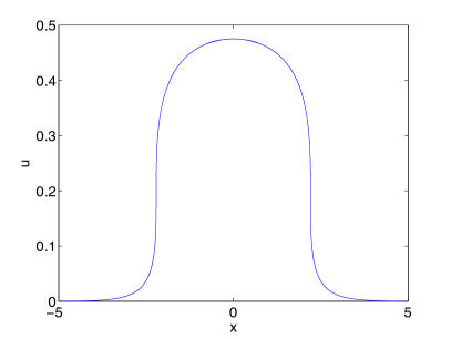
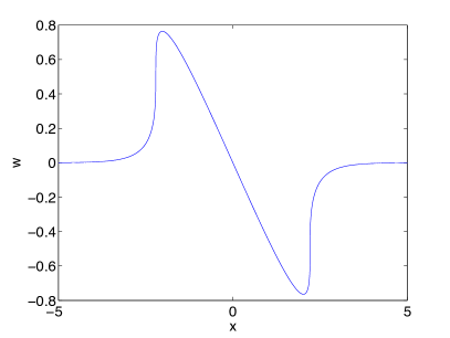
Fig. 1: Solution to the defocusing semiclassical system (4) for the initial data $u_{0}(x)=sech^{2}(x),\,\,w_{0}(x)=0$ at the critical time $t_{c}$; the function $u$ on the left and the corresponding function $w$ on the right.

We consider the initial data (20) since they can be treated analytically, see [19], and thus provide a strong test for our methods. A problematic aspect of these data is that two singularities form at the same time $t_{c}$ at $\pm x_{c}$. Since the contribution of each singularity in the complex plane to the asymptotic behavior of the Fourier coefficients (11) is given by a sum over all singularities, and since the two hitting the real axis at $t_{c}$ differ only in the parameter $\alpha_{j}=\pm x_{c}$, the Fourier coefficients are proportional to $\cos(x_{c}k)$. Thus there are strong oscillations in the coefficients, see Fig. 2 which both affect the accuracy of the solution and impose some potential problems on the asymptotic fitting of the Fourier coefficients. The fitting of $\ln|\hat{u}|$ to (1) is done for $10<k<\max(k)*2/3$. We find the fitting parameters (13) to be $\delta=-3*10^{-5}$, $B=1.3426$, both very close to the theoretical values $0$ and $4/3$, and $A=-6.2224$. Thus the oscillations do not affect the quality of the fitting, but rule out the norm of the difference between $\ln|\hat{u}|$ and the fitted curve (13) as an indicator of the quality of the fitting, as was possible in the examples considered for the Hopf equation in [34]. The results of an analogous fitting for $\ln\hat{w}$ are almost identical indicating that both functions have a cubic singularity. Fitting the imaginary part of $\ln\hat{u}$ according to (14), we find $\alpha=2.5281$ compared to $x_{c}\sim 2.21$.

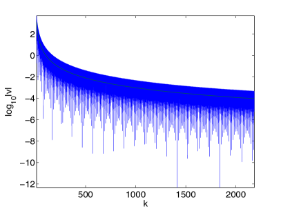
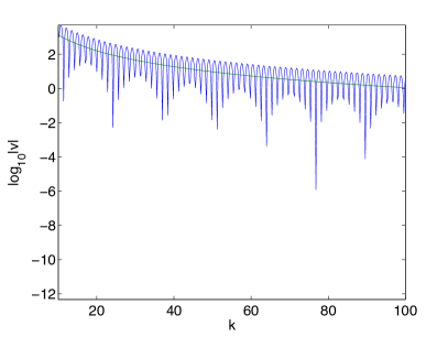
Fig. 2: Modulus of the Fourier coefficients of the solution to the defocusing semiclassical system (4) for the initial data $u_{0}(x)=sech^{2}(x),\,\,w_{0}(x)=0$ at the critical time $t_{c}$ in blue and the fitted curve (13); a close-up of the curve close to the origin is shown on the right.

To check the quality of the numerical solution in Fig. 1, we compare it to the exact solution to the system (21) which can be computed in principle with machine precision. It can be seen in Fig. 3, where the vicinity of $-x_{c}$ is shown, that this difference is largest near the critical point where it is of the order of $10^{-3}$. We conclude that the solution to the semiclassical system can be obtained numerically with a precision of the order of $10^{-3}$ at the critical time, and that the fitting for the Fourier coefficients can be done with a similar accuracy. The difference of the fitting curve and the Fourier coefficients cannot be used as an indicator here since two singularities form at the same time which leads to the oscillations in the Fourier coefficients in Fig. 2.

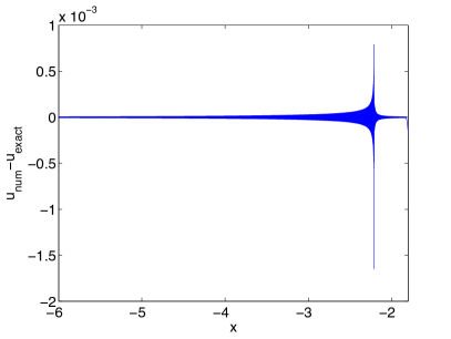
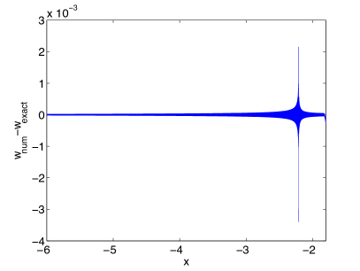
Fig. 3: Difference of the numerical and the exact solution to the defocusing semiclassical system (4) for the initial data $u_{0}(x)=sech^{2}(x),\,\,w_{0}(x)=0$ at the critical time $t_{c}$; for the function $u$ on the left and for the corresponding function $w$ on the right.

3.1.2 Focusing case

For the focusing case we will again consider the initial data (20) for which an exact solution to the focusing cubic NLS was given by Satsuma and Yajima [53] for a sequence of positive values $\epsilon_{N}$ converging to 0. In [3], an exact solution of the modulation equations for these data was given. More precisely, the system (4) was introduced there as a model for the self-focusing phenomenon in one transverse dimension. A system of two real equations was given implicitly defining two real unknowns as functions of $x$ and $t$, and leading to the formation of a finite-amplitude singularity (i.e., a gradient catastrophe) at the time $t=t_{c}=\frac{1}{2A_{0}}$. These data were also studied in [29] for the semiclassical limit of the focusing NLS and numerically in [48]. In [18], the system (4) was reduced to a linear equation by hodograph techniques. For generic localized analytic initial data, the solutions of this system have an elliptic umbilic singularity. For symmetric initial data of the form (20), the solution of the focusing system (4) can be found by solving the system,

$$\left\{\begin{array}[]{ccc}x&=&wt+f_{u},\\ 0&=&ut+f_{w},\end{array}\right.$$ (22)

for $u=u(x,t)$ and $w=w(x,t)$, where $f(u,w)$ has the explicit form

$$f(u,w)=\mbox{Re}\left[\begin{array}[]{c}\left(-\frac{w}{2}+iA_{0}\right)\sqrt{u+\left(-\frac{w}{2}+iA_{0}\right)^{2}}\\ \hskip 85.35826pt+u\log\frac{\left(-\frac{w}{2}+iA_{0}\right)+\sqrt{\left(-\frac{w}{2}+iA_{0}\right)^{2}+u}}{\sqrt{u}}\end{array}\right].$$ (23)

The critical point is given by

$$u_{c}=2A_{0},\,\,\,w_{c}=0,\,\,\,x_{c}=0,\,\,\,t_{c}=\frac{1}{2A_{0}}.$$ (24)

Near the critical point $x_{c}$ for the critical time $t_{c}$, the solution has a cusp, $u(x)\sim|x|^{1/2}$ and $w(x)\sim\mbox{sign}(x)|x|^{1/2}$.

For initial data of the form (20) with $A_{0}=2$, the computation is carried out with $2^{14}$ points for $x\in[-5\pi,\,5\pi]$ and with a time step $\Delta_{t}=2.5*10^{-5}$. The solution at the time $t_{c}=0.25$ can be seen in Fig. 4. The numerically computed energy is conserved to the order of $10^{-14}$. It can be seen that the maximum at the cusp is not fully reached by the numerical solution (its maximum is roughly $7.62$ instead of 8). Note that this does not change much if a higher resolution in Fourier space is used (we reach $7.64$ with $2^{16}$ Fourier modes).

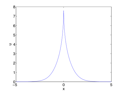
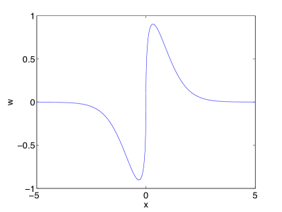
Fig. 4: Solution to the focusing semiclassical system (4) for the initial data $u_{0}(x)=4sech^{2}(x),\,\,w_{0}(x)=0$ at the critical time $t_{c}=0.25$; the function $u$ on the left and the corresponding function $w$ on the right.

In Fig. 5 we show a close-up of the numerical and the exact solution obtained by inverting (22). It can be seen that the agreement is excellent except for the immediate vicinity of the cusp, where there is only a small difference for $w$ which vanishes at the critical point for symmetry reasons, but a more pronounced one for $u$.

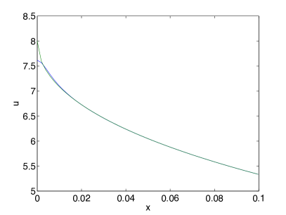
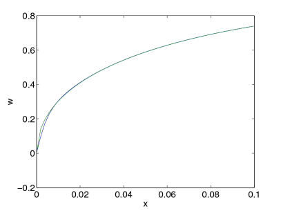
Fig. 5: Close-up of the situation in Fig. 4 together with the corresponding exact solution in green.

A fitting of the Fourier coefficients according to (13) for $10<k<\mbox{max}(k)/2$ gives $\delta=0.0042$, $B=1.09$ and $A=7.28$, see Fig. 6. Visibly the square root singularity is more difficult to reproduce than the cubic root in the defocusing case. In addition the system (4) can be written in the defocusing case in Riemann invariant form as essentially two equations of Hopf type. Thus we can solve it with the same precision as in [34] for the Hopf equation. In the focusing case, the Riemann invariants are complex, and thus we face a true system in this case. Not surprisingly the cusp is not as well reproduced by the numerics as the cubic root, and this is reflected also by the Fourier coefficients. This is mainly true for the algebraic decrease given by the parameter $B$ (which should be equal to $3/2$) which is always more sensitive to this fitting procedure. In fact the fitting parameters are closer to the theoretically expected ones if the fitting is done for $1<k<\mbox{max}(k)/2$. In this case we get $\delta=0.0038$, $B=1.21$ and $A=-7.77$ for the parameters in (13). The fitting error $\Delta$ is in both cases of the order of $0.4$. A larger lower bound has only little effect on the fitting. Note that the fitting parameters for the Fourier coefficients $\hat{w}$ are very similar to what we get for $\hat{u}$: for $10<k<\mbox{max}(k)/2$ we get $\delta=0.0039$, $B=1.18$ and $A=6.69$, see Fig. 6.

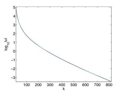
Fig. 6: Modulus of the Fourier coefficients of the solution to the focusing system (4) for the initial data $u_{0}(x)=4sech^{2}(x),\,\,w_{0}(x)=0$ at the critical time $t_{c}=0.25$ in blue and the fitted curve (13); the Fourier coefficients for $u$ on the left, the ones for $w$ on the right.

The difference between the numerical and the exact solution in Fig. 5 is of course the reason that the fitting parameters disagree from the theoretical ones. Since the cusp is formed by the high wave numbers in Fourier space, a discrepancy there affects the asymptotic behavior of the Fourier coefficients as can be seen in Fig. 7; the coefficients agree very well for small wave numbers, but disagree for high wave numbers. Again the agreement is better for $w$ than for $u$. Thus a fitting of the Fourier coefficients of the exact solution to (13) yields $\delta=-0.0007$, $B=1.4935$ and $A=-8.5846$, i.e., very good approximations to the theoretical values. Similarly we get from the fitting of the Fourier coefficients of $w$ the values $\delta=0.0003$, $B=1.4654$ and $A=-7.5718$.

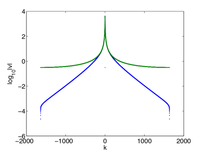
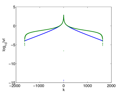
Fig. 7: Modulus of the Fourier coefficients of the solution to the focusing system (4) for the initial data $u_{0}(x)=4sech^{2}(x),\,\,w_{0}(x)=0$ at the critical time $t_{c}=0.25$ in blue and the coefficients of the exact solution in green; the Fourier coefficients for $u$ on the left, the ones for $w$ on the right.

Since the main question in our context is whether the critical time $t_{c}$ can be identified from the asymptotic behavior of the Fourier coefficients, we let the code run until $t=0.255$ with the same parameters as before. The fitting of the Fourier coefficients is done at each time step for $10<k<\mbox{max}(k)/2$. The parameter $\delta$ in (13) vanishes at $t\sim 0.2512$ as can be seen in Fig. 8. The parameter $B$ at this time has the value $1.17$. The solution $u$ at this time can be seen in the same figure. The value of $u$ at the cusp is now roughly $8.5$, thus a bit larger than the correct value of 8. As stated in Remark 4, the smallest distance in the used discrete Fourier space is equal to $2\pi L/N\sim 0.0019$. In principle no distance below this threshold can be numerically distinguished from zero. If we stop the code when $\delta<0.0019$, we find a $t_{c}\sim 0.2506$ and a solution $u$ with a maximum of $7.93$, both very close to the theoretical values.

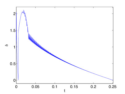
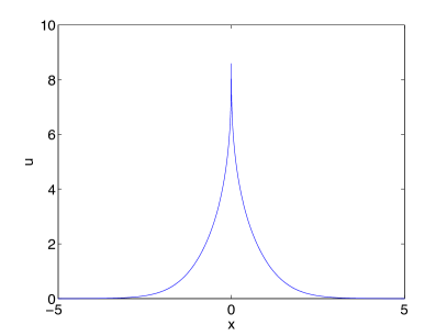
Fig. 8: Fitting parameter $\delta$ of the solution to the focusing system (4) for the initial data $u_{0}(x)=4sech^{2}(x),\,\,w_{0}(x)=0$ in dependence of $t$ on the left, and the solution $u$ at the last time with positive $\delta$ on the right.

The difference between the defocusing and focusing case appears to be in the hyperbolicity respectively ellipticity of the semiclassical system. In the former case we can integrate up to a vanishing of the fitting parameter $\delta$ in (13), and both the critical time and solution are well approximated. In the latter case the ellipticity of the system implies the modulation instability which leads in particular to a pollution of the high wavenumbers. Since in addition the singularity is of higher order in this case (square root instead of cubic), we cannot get as close as in the hyperbolic case to the critical time. Thus the code has to be stopped as soon as $\delta$ is of the order of the smallest distance in Fourier space. This gives a slightly less accurate, but still satisfactory approximation to the critical time and solution than in the hyperbolic case.

The above example shows in fact that we find a critical time close to the theoretical $t_{c}$ of the gradient catastrophe (24), which indicates the fitting is reliable. However as already pointed out, the accuracy is much lower for the value of $B$ in (13), which is not close to the theoretical one ($1.5$). It was already discussed in [34] that the fitting procedure (13) is much more reliable for the exponential part, i.e., $\delta$ the vanishing of which gives the value of $t_{c}$. But it is less so for the algebraic dependence of the Fourier coefficients on $k$, and it appears that the study of a two components system increases this effect. Since we are mainly concerned about the correct identification of the critical time, this is not a problem in this context.

3.2 Semiclassical DS II system

We consider now the semiclassical DS system (9) which is integrable in the sense of [36].
To check the numerical accuracy, we use the energy,

$$E[u,S](t):=\int_{\mathbb{T}^{2}}\left(u\left(S_{x}^{2}-S_{y}^{2}\right)-\rho\left(u^{2}-2(\mathcal{P}^{2}(u)-2\mathcal{Q}^{2}(u))\right)\right)dxdy.$$ (25)

where $\mathcal{P}$ and $\mathcal{Q}$ are defined in Fourier space by

$$\widehat{\mathcal{P}(f)}=\frac{k_{x}^{2}}{k_{x}^{2}+k_{y}^{2}}\widehat{f}(k_{x},k_{y}),\,\,\,\widehat{\mathcal{Q}(f)}=\frac{k_{x}k_{y}}{k_{x}^{2}+k_{y}^{2}}\widehat{f}(k_{x},k_{y}).$$

To numerically solve the system, we use again a fourth order Runge-Kutta scheme, and a Krasny filter of order $10^{-14}$. In the following, the computations are carried out with $2^{14}\times 2^{14}$ points for $x\times y\in[-5\pi,5\pi]\times[-5\pi,5\pi]$. We always perform an asymptotic fitting of the Fourier coefficients in the $k_{x}$-direction as in [34] for the dKP equation, and in both spatial directions via the energy spectrum $\mathcal{E}(K)$ (15) (see sect. 2). We will denote by $\delta_{1d},B_{1d}$ the fitting parameters resulting from the one-dimensional study, for $ln(\hat{u}(k_{x},0))$ in (13), and by $\delta_{2d},B_{2d}$ those resulting from the two-dimensional study (16). For the one-dimensional fitting, we consider in all cases the following range of the Fourier coefficients: $10<k_{x}<\max(k_{x})/2$, and for the two-dimensional fitting, the corresponding range for $K=\sqrt{|k_{x}|^{2}+|k_{y}|^{2}}$: $\sqrt{|k_{x_{min}}|^{2}+|k_{y_{min}}|^{2}}<K<\sqrt{|k_{x_{max}}|^{2}+|k_{y_{max}}|^{2}}$. For the resolution used, this gives $K_{min}\sim 15$.

We find that the singularities appearing in the solutions are of the same type as above in the case of $1+1$-dimensional NLS equations, i.e., gradient catastrophes in one spatial dimension. Due to the symmetry properties of the studied initial data, these coincide with the coordinate axes (one component of the gradient blows up). In particular we find that

• Solutions to the defocusing variant of the semiclassical DS II equation (9) show the same type of break-up as for the corresponding limit of the $1+1$-dimensional NLS equation: the solutions have two break-up points in each spatial direction (not necessarily on the coordinate axes and at the same time) which are generically of cubic type as for generic solutions to the Hopf equation.

• Solutions of the focusing variant of the semiclassical DS II equation (9) have in general two break-up points of the same type as solutions of the focusing $1+1$-dimensional NLS equation, a square root cusp for each spatial direction. For initial data with a symmetry with respect to an interchange of the spatial coordinates, these cusps appear at the same time and location.

3.2.1 Defocusing case

We first consider the defocusing system (9) $(\rho=1)$ for initial data of the form

$$u(x,y,0)=e^{-2R^{2}},\,\,\mbox{with}\,\,R=\sqrt{x^{2}+y^{2}},\,\,\mbox{and}\,\,S(x,y,0)=0,$$ (26)

which thus correspond to Gaussian initial data for the defocusing DS II equation. The time step is chosen as $\Delta_{t}=6*10^{-5}$. The vanishing of $\delta_{1d}$ in (13) and $\delta_{2d}$ in (16) occur at the same time $t_{c}\sim 0.525$, see Fig. 9.

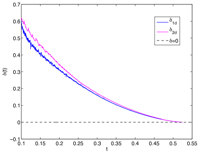
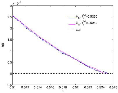
Fig. 9: Time dependence of the fitting parameters $\delta_{1d}$ in (13) and $\delta_{2d}$ in (16) on the left, and for $t$ close to $t_{c}$ on the right, for the numerical solution to the defocusing semiclassical DS II system (9) with initial data (26)

.

We show the solution to the defocusing semiclassical DS II system (9) at this time $t=0.525$ and its Fourier coefficients in Fig. 10.

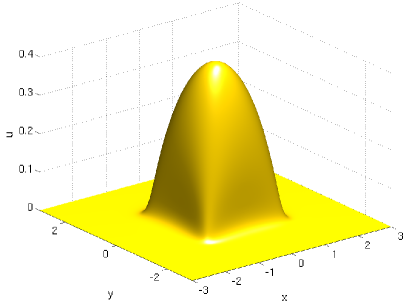
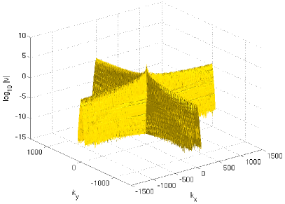
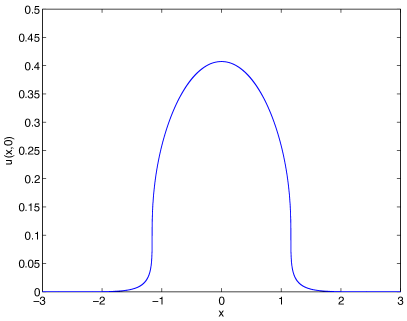
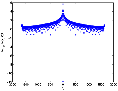
Fig. 10: Numerical solution to the defocusing semiclassical DS II system (9) for initial data (26) at $t=0.525$, and its Fourier coefficients; in the lower row the corresponding figures on the $x$- respectively $k_{x}$-axis are given.

It can be seen that the solution becomes steep on the 4 sides parallel to the coordinate axes, and the $x$-derivative of $u$, respectively the $y$-derivative, become big in two points on the $x$-axis, respectively $y$-axis, namely in $(x_{c}^{\pm}=\pm 1.162,0)$, respectively. $(0,y_{c}^{\pm}=\pm 1.162)$. The other parameters attain the following values at $t=0.525$: $B_{1d}$ (13) reaches $B_{1d}=1.35$, $B_{2d}$ in (16) $\sim 2.99$, and the numerically computed energy (10) $\Delta_{E}=4.5*10^{-14}$. The situation is visibly similar to the $1+1$-dimensional example shown in Fig. 1, just that now four singularities form at the same time for symmetry reasons. This implies as in Fig. 2 strong oscillations in the Fourier coefficients, now both in $k_{x}$ and $k_{y}$ direction. A direct consequence of this is that the fitting errors cannot be used as an indicator of the quality of the fitting (one has $\Delta_{1d}$ of the order of $\sim 5$ and $\Delta_{2d}\sim 1$). But the fitting appears to be very reliable as in the $1+1$-dimensional case which is also confirmed by the value of $B_{1d}\sim\frac{4}{3}$ which again indicates a cubic singularity.

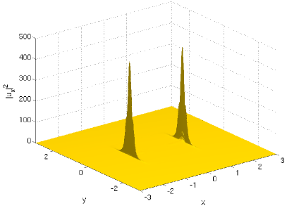
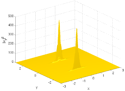
Fig. 11: Derivatives of the numerical solution to the defocusing semiclassical DS II system (9) with initial data (26); $|u_{x}|^{2}$ (left) and $|u_{y}|^{2}$ (right) at $t=0.525$.

The results of this subsection can be summarized in the following

Conjecture 5.

Solutions to the defocusing semiclassical DS II system (9) for generic rapidly decreasing initial data with a single hump develop four points of gradient catastrophe in finite time. At each of these points, only one component of the gradient becomes infinite. The singularity is thus one dimensional, the solution at these points $x_{c}$ and $y_{c}$ respectively behaves as $(x-x_{c})^{1/3}$ respectively $(y-y_{c})^{1/3}$.

3.2.2 Focusing case

A similar study as above is presented for the focusing ($\rho=-1$) semiclassical DS II system (9), first with non-symmetric initial data

$$u(x,y,0)=e^{-2R^{2}},\,\,\mbox{with}\,\,R=\sqrt{x^{2}+0.1y^{2}},\,\,\mbox{and}\,\,S(x,y,0)=0.$$ (27)

The time step is chosen as $\Delta_{t}=3*10^{-5}$. The vanishing of $\delta_{1d}$ in (13) and $\delta_{2d}$ in (16) occur in this case roughly at the same time, $t_{c}\sim 0.1946$, see Fig. 12.

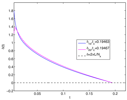
Fig. 12: Time dependence of the fitting parameter $\delta$ for the numerical solution to the focusing semiclassical DS II system with initial data (27)

The solution to the focusing semiclassical DS II system (9) at $t=0.1946$ and its Fourier coefficients can be seen in Fig. 13.

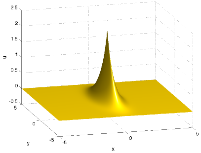
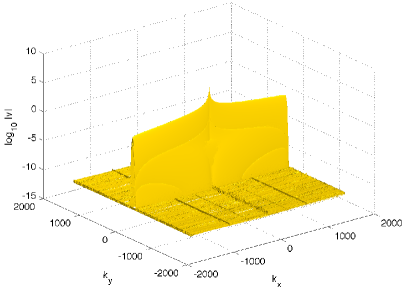
Fig. 13: Numerical solution to the focusing semiclassical DS II system (9) with initial data (27) at $t=0.1946$ on the left, and its Fourier coefficients on the right.

Visibly the solution develops a cusp in the $x$-direction at $t_{c}$, which is also reflected by both $\delta_{1d}$ and $\delta_{2d}$ vanishing. The parameter $B_{1d}$ in (13) reaches a value of $B_{1d}(t_{c})\sim 1.24$ and $B_{2d}(t_{c})\sim 2.77$ in (16). As in the $1+1$-dimensional case we thus do not recover a value of $B_{1d}$ close to $1.5$, but we get essentially what was observed there. One can conclude that the solution at the critical point has a square root type cusp. Presumably a second such cusp would form at a later time in $y$-direction if the code could be run beyond the first critical time.

At $t=t_{c}$, the $x$-gradient of $u$ begins to explode, with $\|u_{x}\|_{\infty}\sim 30$, see Fig. 14, where we show $|u_{x}|^{2}$ on the left and $|u_{y}|^{2}$ on the right. We observe that the gradient catastrophe only appears in one spatial point, $(x_{c},y_{c})$, here $(0,0)$. The fitting error $\Delta_{1d}$ is of the order $0.2$ which is again similar to what was observed in the $1+1$-dimensional case, and $\Delta_{2d}\sim 2$ at $t_{c}$.

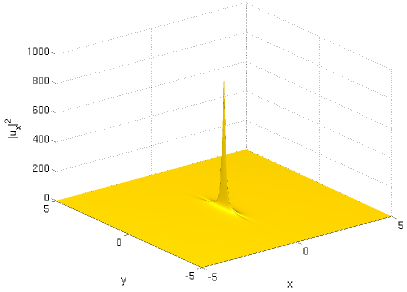
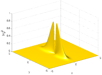
Fig. 14: Derivatives of the numerical solution to the focusing semiclassical DS II system (9) with initial data (27), $|u_{x}|^{2}$ (left) and $|u_{y}|^{2}$ (right) at $t=0.1946$.

The situation is quite different if we consider symmetric initial data,

$$u(x,y,0)=e^{-2R^{2}},\,\,\mbox{with}\,\,R=\sqrt{x^{2}+y^{2}},\,\,\mbox{and}\,\,S(x,y,0)=0.$$ (28)

In this case a cusp occurs in both spatial directions at the same time, as can be seen in Fig. 15. There we show the solution to the focusing semiclassical DS II system (9) with initial data (28) at $t=t_{c}$, the latter being determined, as before, by using a fitting for the asymptotic behavior of the Fourier coefficients.

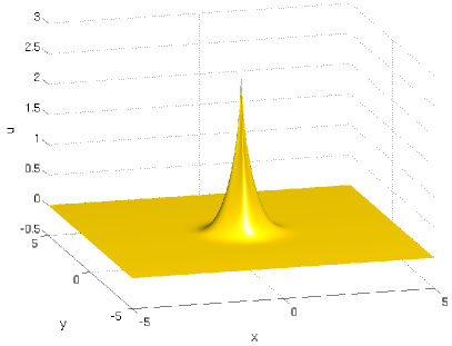
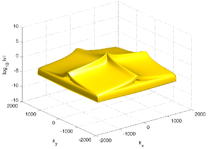
Fig. 15: Numerical solution to the focusing semiclassical DS II system (9) with initial data (28) at $t=0.2153$, and its Fourier coefficients.

The bounds for the fitting are chosen as previously and yield a vanishing of $\delta_{1d}$ in (13) and $\delta_{2d}$ in (16) at roughly the same time $t_{c}\sim 0.2153$, see Fig. 16.

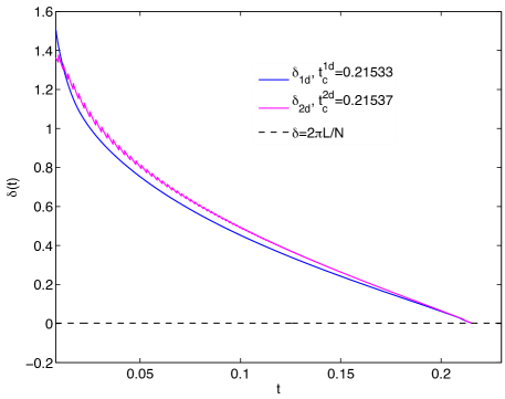
Fig. 16: Time dependence of the fitting parameter $\delta$ for the numerical solution to the focusing semicalssical DS II system (9) with initial data (28).

The parameter $B_{1d}$ (13) reaches a value of $B_{1d}\sim 1.21$ at this time, and $B_{2d}\sim 2.55$ (16). The fitting errors are roughly of the same order as in the previous case, one gets $\Delta_{1d}\sim 0.3$ and $\Delta_{2d}\sim 0.7$. The $L_{\infty}$-norm of $u_{x}$ clearly explodes with $\|u_{x}\|_{\infty}\sim 35$, as well as the $L_{\infty}$-norm of $u_{y}$ which reaches the same value. We show in Fig. 17 the $x$- and $y$-derivatives of $u$.

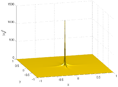
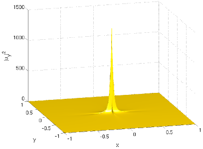
Fig. 17: Derivatives of the numerical solution to the focusing semiclassical DS II system with initial data (28), $|u_{x}|^{2}$ (left) and $|u_{y}|^{2}$ (right) at $t=0.2153$.

The results of this subsection can be summarized in the following

Conjecture 6.

Solutions to the focusing semiclassical DS II system (9) for generic rapidly decreasing initial data with a single hump develop two points of gradient catastrophe in finite time. At each of these points only one component of the gradient is unbounded. The singularity is thus one dimensional, the solution at these points $x_{c}$ and $y_{c}$ respectively behaves as $(x-x_{c})^{1/2}$ respectively $(y-y_{c})^{1/2}$. If the initial data are invariant under an exchange of $x$ and $y$, these two points coincide.

4 Semiclassical Limit of Davey-Stewartson II solutions

In this section, we numerically study solutions to the DS II equation for the initial data of the previous section for several values of $\epsilon\ll 1$. We then investigate the scaling laws, i.e, the dependence on $\epsilon$ of the difference between the DS II and semiclassical DS II solutions. In the previous section we had shown that the singularities of the semiclassical DS II system are as in the corresponding $1+1$ dimensional situations. The same is observed for the dispersive regularizations near the singularity here, i.e., for the difference of semiclassical DS II and DS II solutions for finite small $\epsilon$, both for the same initial data: we find the same scalings in $\epsilon$ as in the $1+1$ dimensional case, $\epsilon^{2/7}$ for the defocusing case and $\epsilon^{2/5}$ for the focusing case.

4.1 Defocusing case

We consider zero initial phase data of the form

$$\Psi_{0}(x,y)=e^{-R^{2}},\,\,R=\sqrt{x^{2}+y^{2}},$$ (29)

which correspond to the initial data (26) studied before for the defocusing semiclassical DS II system (9), now for defocusing DS II ((6) with $\rho=1$). The computations are carried out with $N_{x}=N_{y}=2^{14}$ Fourier modes, $L_{x}=L_{y}=5$, and $\Delta_{t}=2*10^{-4}$ for different values of $\epsilon$, until $t_{max}=1$, almost twice the critical time of the corresponding semiclassical system identified in Sec. 3.2.1.

The defocusing effect of the equation for these initial data can be seen in Fig. 18, where $|\Psi|^{2}$ is shown for several values of $t$. The compression of the initial pulse into some almost pyramidal shape leads to a steepening on the 4 sides orthogonal to the coordinate axes and to oscillations at the bottom edges of the ‘pyramid’, see also [33].

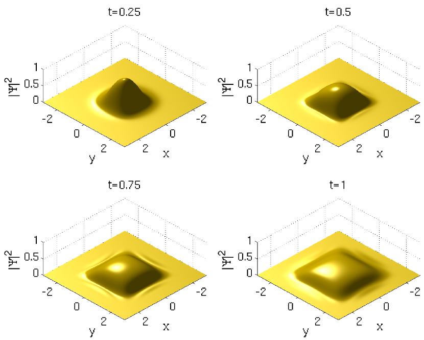
Fig. 18: Solution to the defocusing DS II equation for the initial data (29) and $\epsilon=0.1$ for several values of $t$.

The situation is similar for smaller values of $\epsilon\in[0.005,0.1]$. The oscillations become more rapid and more confined to a zone the smaller $\epsilon$ is, as can be seen in Fig. 19, where we show the square of the absolute value of $\Psi(x,0,t)$ in dependence of $x$ at $t_{max}=1$ for different values of $\epsilon$. It can be seen that a lens shaped zone forms in the vicinity of each of the shocks of the semiclassical DS II system which should delimit for $\epsilon\to 0$ the oscillations.

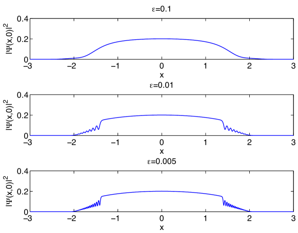
Fig. 19: Absolute value of the numerical solutions of the defocusing DS II for the initial data (29) for $y=0$ and $t=1$ for different values of $\epsilon$.

A contour plot for the modulus squared of these solutions can be found in Fig. 20.

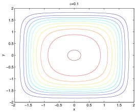
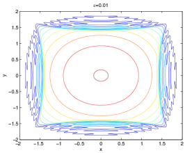
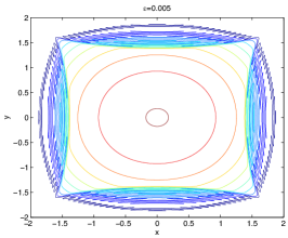
Fig. 20: Contour plot of $|\Psi|^{2}$ for solutions of the defocusing DS II equation for the initial data (29) at $t=1$ for different values of $\epsilon$.

We ensure that the system is well resolved numerically by checking both the decay of the Fourier coefficients, which decrease here to machine precision, see Fig. 21, and also the time evolution of the quantity $\Delta_{E}$ (10). The numerically computed energy $E[\Psi](t)$, which is a conserved quantity of DS (7) for the exact solution, is here evaluated on $\mathbb{T}^{2}$. The quantity $\Delta_{E}$ increases due to unavoidable numerical errors, but stays below $10^{-8}$ until the end of the computation for all studied cases. This is of the same order as the results for the semiclassical limit of the defocusing NLS equation in [7, 28, 31].

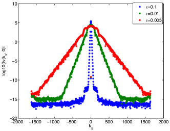
Fig. 21: Modulus of the Fourier coefficients for the solutions in Fig. 19, plotted on the $k_{x}$-axis at the maximal time of computation, $t_{max}=1$ for different values of $\epsilon$.

An important question is the scaling with $\epsilon$ of the $L_{\infty}$ norm of the difference between semiclassical DS II and DS II solutions for the same initial data. The $L_{\infty}$ norm of this difference is shown in Fig. 22 at the critical time $t_{c}=0.525$ in dependence of $\epsilon$ for $0.01\leq\epsilon\leq 0.1$.

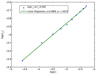
Fig. 22: $L_{\infty}$ norm $\Delta_{\infty}$ of the difference between defocusing DS II solutions and the solutions to the defocusing system (9) for the initial data (29), respectively (26) in dependence of $\epsilon$ at $t_{c}=0.525$.

A linear regression analysis ($\log_{10}\Delta_{\infty}=a\log_{10}\epsilon+b$) shows that $\Delta_{\infty}$ decreases as

$$\mathcal{O}\left(\epsilon^{0.28}\right)\sim\mathcal{O}\left(\epsilon^{2/7}\right)\,\,\mbox{at}\,\,t=t_{c}=0.525,\,\,\mbox{with}\,\,a=0.2868\,\,\mbox{and}\,\,b=-1.9972.$$ (30)

The correlation coefficient is $r=0.998$.

This means that the same scaling is found as in the defocusing NLS case for which an asymptotic description at break-up was conjectured in [19]. Thus it appears that the essentially one-dimensional character of the singularity of the solution of the semiclassical DS II system (9) implies that the regularization effect of the dispersion in the full DS II system is as in the $1+1$-dimensional case. It has to be checked whether the special PI2 solution appearing in the asymptotic description of the NLS solution near the critical point plays a role also in the $2+1$-dimensional case.

4.2 Focusing case

We consider now solutions of the focusing DS II equation for small $\epsilon$. The initial condition corresponding to (27) is

$$\Psi_{0}(x,y)=e^{-R^{2}},\,\,\mbox{with}\,\,R=\sqrt{x^{2}+0.1y^{2}}.$$ (31)

For $\epsilon=0.1$, the computation is carried out with $2^{14}\times 2^{14}$ points for $x\times y\,\in\,[-5\pi,5\pi]\times[-5\pi,5\pi]$, and $\Delta_{t}=8*10^{-5}$. For smaller values of $\epsilon$, we take $N_{x}=N_{y}=2^{15}$ to ensure sufficient resolution in Fourier space up to the maximal time of computation $t_{max}$. The latter is chosen to be $t_{max}=0.5$, almost twice the break-up time of the corresponding focusing semiclassical DS II system found in sect. 3.2.2.

For $\epsilon=0.1$, the initial peak grows until its maximal height (here $\sim 3.24$) at $t\sim 0.275$. At later times it breaks up into smaller humps, see Fig. 23 as in the case of the one-dimensional cubic NLS equation in the semiclassical limit, see for instance [31, 18].

Fig. 23: Modulus of the solution to the focusing DS II equation with initial data (31) and $\epsilon=0.1$ at several times.

The Fourier coefficients decrease to machine precision at $t_{max}=0.5$ as can be seen in Fig. 24, and the numerically computed energy is of the order $\Delta_{E}\sim 1.5*10^{-11}$ at this time.

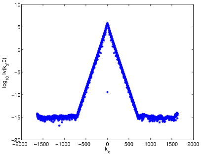
Fig. 24: Modulus of the Fourier coefficients of the solution shown in Fig. 23 at $t=0.5$ on the left, and plotted on the $k_{x}$-axis on the right.

The situation is similar for smaller values of $\epsilon$, we observe as expected an increase of the number of oscillations in the dispersive shock as can be seen in Fig. 25, where we show the contour plots of the solutions of the focusing DS II equation at $t=t_{max}=0.5$ with initial data (31) for different values of $\epsilon$. Again the oscillations of appear to be more and more confined for smaller $\epsilon$ to a lense shaped zone.

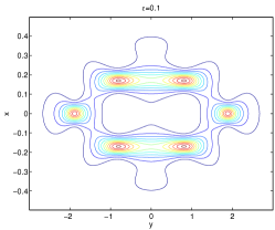
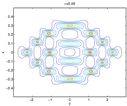
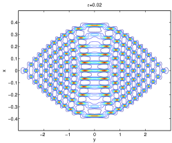
Fig. 25: Contour plots of the numerical solutions of the focusing DS II equation at $t=t_{max}=0.5$ with initial data (31) for different values of $\epsilon$.

For all situations studied, we check the decay of the Fourier coefficients up to $t_{max}$, and the precision indicated by $\Delta_{E}$. We can see in Fig. 26, that for the situations shown in Fig. 25, the Fourier coefficients decrease to machine precision for $\epsilon=0.06$. For $\epsilon=0.02$, the phenomenon of modulational instability leads to a slight increase of the latter for high wave numbers, but they still decrease to $10^{-10}$, which is more than satisfactory here. This is of course due to the high spatial resolution used in the simulations and shows why such a resolution is needed here. At $t=t_{max}$, the numerically computed energy is of the order of $\Delta_{E}\sim 5.7*10^{-11}$ for the case $\epsilon=0.06$ and $\Delta_{E}\sim 1.5*10^{-7}$ for the case $\epsilon=0.02$. This indicates a numerical error well below plotting accuracy.

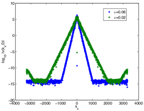
Fig. 26: Fourier coefficients of the solutions shown in Fig. 25 at $t=0.5$ plotted on the $k_{x}$-axis for $\epsilon=0.06$ and $\epsilon=0.02$.

In [40], the semiclassical limit of the $1+1$-dimensional focusing cubic NLS equation is studied. It is shown that near the point of gradient catastrophe $(x_{c},t_{c})$, each spike of the NLS solutions is asymptotically described by the Peregrine breather, an exact rational solution to NLS, and has the height $3|u^{\epsilon}(x_{c},t_{c})|$. The authors illustrated numerically this relation for $\epsilon=\frac{1}{33}$. Here, we have determined in Section 3.2.2 the break-up time numerically with some potential small error, and it is not clear whether a similar relation holds also for DS II. Nevertheless, we compare in Table 1 the values of $|\Psi^{\epsilon}(x_{c},t_{c})|$ and $|\Psi^{\epsilon}(x_{c},t_{peak})|$, where $t_{peak}$ corresponds to the time, where the first spike appears in the numerical solution, before the appearance of oscillations. We find that as $\epsilon$ decreases, the ratio $\frac{|\Psi^{\epsilon}(x_{c},t_{peak})|}{|\Psi^{\epsilon}(x_{c},t_{c})|}$ tends also here to $3$.

$\epsilon$	$0.1$	$0.06$	$0.04$	$0.02$
$\frac{|\Psi^{\epsilon}(x_{c},t_{peak})|}{|\Psi^{\epsilon}(x_{c},t_{c})|}$	$2.5807$	$2.7772$	$2.8792$	$2.9811$

Table 1: Ratio $\frac{|\Psi^{\epsilon}(x_{c},t_{peak})|}{|\Psi^{\epsilon}(x_{c},t_{c})|}$ for several values of $\epsilon$ for initial data of the form (27).

Remark 7.

If one considers initial data of the form $\Psi_{0}(x,y)=e^{-R^{2}},\,\,\mbox{with}\,\,R=\sqrt{x^{2}+\nu y^{2}},$ and $\nu<1$, the situation is similar. We observe the appearance of dispersive shocks, and as $\epsilon$ decreases, the number of oscillations increases. The ratio $\frac{|\Psi^{\epsilon}(x_{c},t_{peak})|}{|\Psi^{\epsilon}(x_{c},t_{c})|}$ tends also to $3$ as $\epsilon$ tends to $0$ for other values of $\nu<1$.

We now study the scaling of the difference of the DS II and the semiclassical DS II solution for the initial data (26), at $t=t_{c}=0.1946$, for different values of $\epsilon$. We consider values of $\epsilon$ between $0.1$ and $0.01$, with $N_{x}=N_{y}=2^{14}$. Note that we use here less resolution since the maximal time of computation is $t_{c}\sim 0.1946$, and that the modulational instability and other typical numerical problems are due to the formation of dispersive shocks. Thus we do not need the high spatial resolution we used before for the study in the semiclassical limit.

At $t_{c}\sim 0.1946$, the $L_{\infty}$ norm of the difference between semiclassical DS II and DS II solutions for the same initial data roughly decreases as $\mathcal{O}\left(\epsilon^{0.45}\right)$. Indeed, by doing a linear regression analysis ($\log_{10}\Delta_{\infty}=a\log_{10}\epsilon+b$), we find $a=0.4562$, $b=0.2946$ and $r=0.999$, ($r$ being the correlation coefficient) as can be seen in Fig. 27.

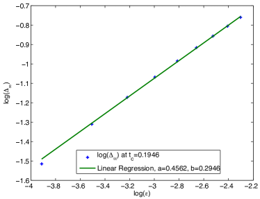
Fig. 27: $L_{\infty}$ norm $\Delta_{\infty}$ of the difference between focusing DS II solution and the corresponding solution to the focusing semiclassical DS II system (9) for the initial data (27) respectively (26) in dependence of $\epsilon$ at $t_{c}=0.1946$.

The scaling at the break up time is similar for a symmetric initial data of the form

$$\Psi_{0}(x,y)=e^{-R^{2}},\,\,\mbox{with}\,\,R=\sqrt{x^{2}+y^{2}},$$ (32)

i.e., the second case studied in Sec. 3.2.2. For $0.1\leq\epsilon\leq 0.02$, we find that the $L_{\infty}$-norm of the difference between the solutions to the focusing DS II and the corresponding system (9) at $t_{c}=0.2153$ scales as $\epsilon^{0.4}$. The situation is shown in Fig. 28, for which a linear regression ($\log(\Delta_{\infty})=a\log(\epsilon)+b$) gives $a=0.4018$, $b=0.8911$ and $r=0.999$. Note that this is the same scaling conjectured in the focusing NLS case, see [19] for an asymptotic description at break-up. In the asymptotic description of the critical behavior of $1+1$-dimensional focusing NLS solutions, the tritronquée solution of the PI equation appeared. It remains to be checked whether this solution also plays a role in the context of the focusing DS II equation.

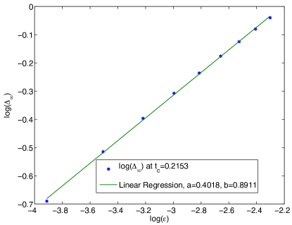
Fig. 28: $L_{\infty}$-norm of the difference between the solutions to the focusing DS II solution and the corresponding solution to the focusing semiclassical DS II system for symmetric initial data at $t_{c}=0.2153$ in dependence of $\epsilon$.

Since in [52], preliminary results in this context suggest that for symmetric initial data, the solutions of the DS II equation in the semiclassical limit blow up for larger $t$, we study this special case in the following section.

5 Blow-up in solutions to the Davey-Stewartson II equations in the semiclassical limit

In this section we study numerically the possibility of a blow-up in solutions to the focusing DS II system in the small dispersion limit. Since the formation of a dispersive shock implies that the initial peak decomposes into smaller ones, a blow-up appears only to be possible if the initial hump continues to grow without limits. In this sense blow-up and dispersive shocks appear to be competing phenomena. In the examples studied in the previous section, there is clearly no blow-up. To identify numerically a potential blow-up, we will use again the asymptotic behavior of the Fourier coefficients to indicate as for the semiclassical systems the appearance of this singularity by the vanishing of $\delta$, i.e., the disappearance of the exponential decay of the coefficients. We first test this approach for the $1+1$-dimensional focusing quintic NLS equation, for which previous studies of blow-up exist, see for instance [56] for a review of the topic and references. Then we investigate this phenomenon for the semiclassical DS II system for initial data with a symmetry with respect to an exchange of $x$ and $y$. We find that there is indeed a blow-up in this case, and that the difference between break-up and blow-up time scales roughly as $\epsilon$ (the corresponding scaling in the $1+1$-dimensional case is $\epsilon^{4/5}$).

5.1 Focusing Quintic NLS Equation

We first consider the quintic NLS equation to check the efficiency of our methods to detect blow-up phenomena. It is well known that solutions to focusing NLS equations of the form (1) can have blow-up, if $\sigma d\geq 2$. Thus the simplest case to investigate blow-up phenomena for 1+1-dimensional focusing NLS equations is $\sigma=2$, i.e., the focusing quintic NLS equation,

$$i\epsilon\Psi_{t}+\frac{\epsilon^{2}}{2}\Psi_{xx}+\frac{1}{2}|\Psi|^{4}\Psi=0.$$ (33)

It is well known (see [47]), that its solutions can blow up in finite time for initial data with negative energy $E[\Psi]$,

$$E[\Psi]=\int_{\mathbb{R}}\left(\frac{\epsilon^{2}}{2}|\partial_{x}\Psi|^{2}-\frac{|\Psi|^{6}}{6}\right)dx.$$ (34)

In the semiclassical regime ($\epsilon\to 0$), this condition is obviously met for arbitrary non trivial initial data in $L_{2}$ for sufficiently small $\epsilon$.

We study here two situations where a blow-up occurs in the solutions to this equation. First, we look at an example for $\epsilon=1$ studied in [55] and in [32] for the initial data $\Psi_{0}(x)=1.8i\exp(-x^{2})$ having negative energy. Since we aim to study the semiclassical limit of the Davey-Stewartson system, where blow-up is expected to appear for special classes of initial data, see [52], we also consider a typical example in the semiclassical limit to the quintic NLS equation with initial data of the form $\Psi(x,0)=\mbox{sech}\,x$ and $\epsilon=0.1$.

In the first experiment, ($\Psi_{0}(x)=1.8i\exp(-x^{2})$, $\epsilon=1$), the computation is carried out with $2^{14}$ Fourier modes for $x\in[-5\pi,5\pi]$, and the fitting of the Fourier coefficients is done for $5<k<\max(k)/2$. This case has been studied in [55] and the blow-up time $t^{*}$ has been identified. Note however, that in this paper, they considered the following form of the quintic NLS equation,

$$i\epsilon\Psi_{t}+\epsilon^{2}\Psi_{xx}+|\Psi|^{4}\Psi=0,$$ (35)

i.e., the change of $t\to t/2$ in (33). To compare our result with the ones of [55], we thus consider this form of the equation for the first experiment. With this time scale, the blow-up time $t^{*}$ has been identified in [55] to be $t^{*}\sim 0.135$.

We recover exactly this value from the fitting of the Fourier coefficients, see Fig. 29, where we show the time dependence of the fitting parameter $\delta$ (13).

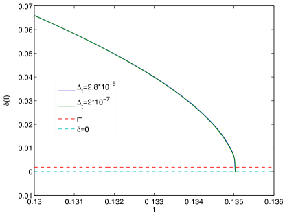
Fig. 29: Time dependence of the fitting parameter $\delta$ (13) for $t$ close to the blow-up time $t^{*}$ for the numerical solution to the focusing $1+1$-dimensional quintic NLS equation with $\epsilon=1$ and initial data $\Psi_{0}(x)=1.8i\exp(-x^{2})$. The fitting is done for $5<k<\max(k)/2$.

We can see that $\delta$ (13) decreases rapidly as expected and vanishes at $t^{*}\sim 0.135$. In addition, we can roughly determine via the fitting parameter $B$ (13) that the singularity corresponds to a blow-up here. Indeed for $t$ approaching the blow-up time, the parameter $B$ stays close to $0.5$, corresponding to a $1/\sqrt{x}$ singularity as actually expected, before decreasing rapidly, see Fig. 30. The reason for this behavior is obviously the blow-up which completely destroys the Fourier coefficients. This can be also seen from the fitting error which increases at the same time, see also Fig. 30.

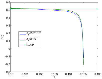
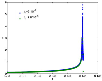
Fig. 30: Time dependence of the fitting parameter $B$ (13) and of the fitting error $\Delta$ (13) for the numerical solution to the focusing $1+1$-dimensional quintic NLS equation with $\epsilon=1$ and initial data $\Psi_{0}(x)=1.8i\exp(-x^{2})$.

A mesh refinement close to the blow up time does not reduce this behavior, as we can infer from the previous pictures, where we show the time evolution of $\delta$, $B$ (13) and of $\Delta$ for $t\sim t^{*}$ for two different mesh sizes. In the first case, $\Delta_{t}=2.8*10^{-5}$, and in the second case, $\Delta_{t}=2*10^{-7}$. In the latter case, the loss of precision in $\Delta$ is clearer, and the value of $B$ stays longer close to $0.5$. But it appears not worth to use such a high resolution, which is computationally expensive, since it does not have an influence on the quantities as $t^{*}$ we are interested in, and this is even more true for the second experiment below. The fact that the results essentially do not change if higher resolution is used clearly confirms that blow-up occurs. But close to $t^{*}$, phenomena as the rapid decrease of $B$ and the loss of precision of $\Delta$ cannot be avoided.

The situation is rather similar for the experiment in the semiclassical limit. We consider here initial data of the form $\Psi(x,0)=\mbox{sech}\,x$, $\epsilon=0.1$ and $2^{15}$ Fourier modes for $x\in[-10\pi,10\pi]$. We find that the blow-up occurs at $t^{*}\sim 0.5455$ as already observed in [19]. We show the time evolution of the fitting parameters in Fig. 31 together with the time evolution of the fitting error $\Delta$, again for two different mesh sizes.

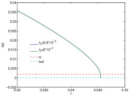
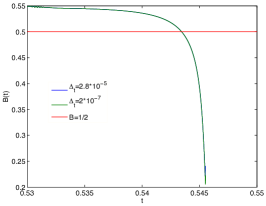
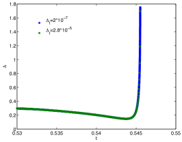
Fig. 31: Time dependence of the fitting parameters $\delta$ and $B$ (13) and of the fitting error $\Delta$ for $t$ close to $t^{*}$ for the numerical solution to the focusing $1+1$-dimensional quintic NLS equation with $\epsilon=0.1$ and initial data $\Psi_{0}(x)=\mbox{sech}\,x$. The fitting is done for $5<k<\max(k)/2$

The parameter $B$ (13) once more decreases rapidly close to the blow-up time, and the fitting error increases there. In this case, a mesh refinement close to $t^{*}$ does not have any influence.

In both cases, we find, however, that the critical time can be roughly recovered from the fitting of the Fourier coefficients. The type of the singularity, here a blow-up, can also be identified via the value of $B$ close to $0.5$ before the blow-up time. Typically, a fitting error smaller than $0.5$ can be achieved before the blow-up time, where the latter diverges. This is a noticeable difference to the case of a singularity with finite $L_{\infty}$ norm (see section 3, and also [34]), where we did not observe such a behavior.

5.2 Symmetric initial data for the DS II equation

We now consider symmetric (with respect to an interchange of $x$ and $y$) initial data of the form

$$\Psi_{0}(x,y)=e^{-R^{2}},\,\,\mbox{with}\,\,R=\sqrt{x^{2}+y^{2}},$$ (36)

for the DS II equation, i.e., the second case studied in Sec. 3.2.2, and $\epsilon=0.1$. As we will see, the behavior of the solutions for this initial condition is similar to the solutions of the $1+1$-dimensional quintic NLS equation in the semiclassical limit above, i.e., a blow-up occurs.
The computation is carried out with $2^{14}\times 2^{14}$ Fourier modes for $x\times y\,\in\,[-5\pi,5\pi]\times[-5\pi,5\pi]$, and $\Delta_{t}=4.5*10^{-5}$. By performing a two-dimensional fit of the Fourier coefficients (16), we find that the solution develops a singularity at time $t^{*}=0.2955$, see Fig. 32. The behavior of $B_{2d}$ is shown in the same figure.

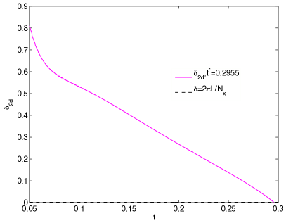
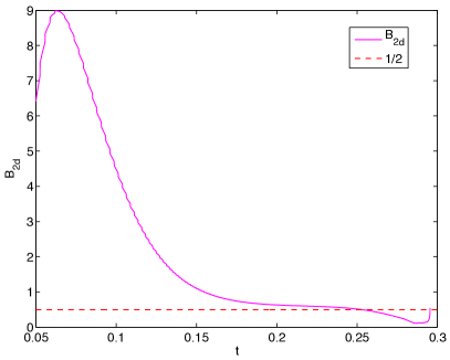
Fig. 32: Time dependence of the fitting parameters $\delta_{2d}$ and $B_{2d}$ in (16) for the solution of the focusing DS II equation with initial data (36) and $\epsilon=0.1$.

The profile of the solution at this time in Fig. 33 also clearly indicates an $L_{\infty}$ blow-up, with $\|u\|_{\infty}\sim 65$, and this is also confirmed by the derivatives of $u$ in Fig. 34, with $\|u_{x}\|_{\infty}\sim\|u_{y}\|_{\infty}\sim 120$.

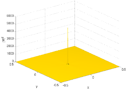
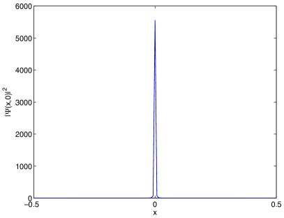
Fig. 33: Square of the absolute value of the solution of the focusing DS II equation with initial data (36) and $\epsilon=0.1$ at $t=0.2955$.

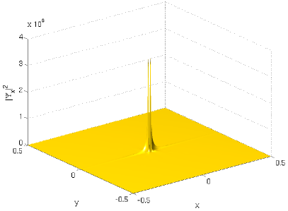
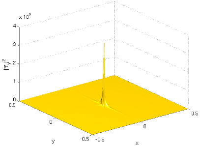
Fig. 34: Derivatives of the solution of the focusing DS II equation with initial data (36) and $\epsilon=0.1$ at $t=0.2955$.

As $\epsilon$ decreases, the blow-up time decreases as well, see Fig. 35, where we show the time dependence of the fitting parameters $\delta_{2d}$ and $B_{2d}$ (16) for several values of $\epsilon\in[0.03,\,0.1]$.

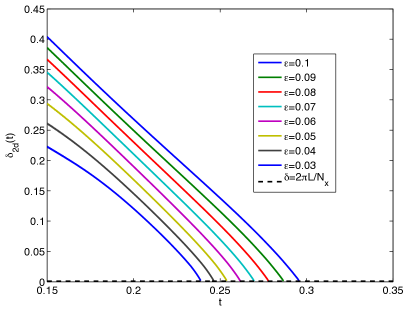
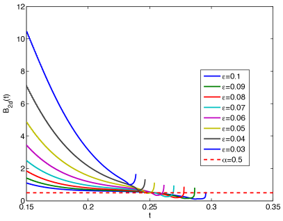
Fig. 35: Time dependence of the fitting parameters $\delta_{2d}$ and $B_{2d}$ (16) for the solution of the focusing DS II equation with initial data (36) for several values of $\epsilon$.

The difference between the blow-up time $t^{*}$ and the corresponding break-up time of the dispersionless system $t_{c}=0.2153$ scales roughly as $\epsilon$, see Fig. 36 (left). Indeed, a linear regression analysis, ($\log_{10}(t^{*}-t_{c})=a\log_{10}\epsilon+b$) gives

$$a=1.0189,\,\,b=-0.1948\,\,\mbox{and}\,\,r=0.999.$$

Since the determination of the blow-up time is numerically delicate, it is difficult to decide whether this scaling is really different from the $\epsilon^{4/5}$ scaling observed for the blow-up in $1+1$-dimensional NLS solutions.

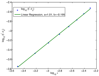
Fig. 36: Difference between the blow-up time $t^{*}$ and the corresponding break-up time of the semicalssical DS II system $t_{c}=0.2153$ in dependence of $\epsilon$

6 Conclusion

In this paper we have shown that important information on the semiclassical limit of the DS II system can be obtained numerically. We considered localized initial data and used the asymptotic behavior of the Fourier coefficients to identify the points of gradient catastrophe in the semiclassical DS II system. This approach was shown to be very efficient for the defocusing semiclassical NLS in $1+1$ dimensions, and within a few percent accuracy for the focusing case.

In both the defocusing and focusing case we observe a hyperbolic blow-up, i.e., a gradient catastrophe at points, where the solution stays finite. In the defocusing case, we find as for the defocusing semiclassical system of the NLS in $1+1$ dimensions a cubic behavior. This means that in our examples, there are four break-up points which due to the symmetry of the initial data were located on the coordinate axes. The break-up at each singular point is such that only one of the derivatives blows up, whereas the other stays finite (here for symmetry reasons, either the $x$- or the $y$-derivative). In the focusing semiclassical DS II system, the break-up is again similar to the $1+1$-dimensional focusing semiclassical NLS system. It appears to be a square root type break-up. For generic initial data, only one of the derivatives (for symmetry reasons they coincide here again with the $x$ and $y$ derivatives) blows up, whereas the other stays finite. But for data with a symmetry with respect to an exchange of $x$ and $y$, these break-ups can happen at the same time and location.

In a second step we solved the DS II equation for some finite small $\epsilon$ for the same initial data as before up to the previously identified critical time. We found that the difference between the semiclassical DS II solution $u_{SC}$, and the DS II system solution $u_{DS}=|\Psi|^{2}$ shows the same scaling in $\epsilon$ as the corresponding $1+1$-dimensional NLS solutions for which an asymptotic description was conjectured in [19]. This means we have in the defocusing case

$$|u_{DS}-u_{SC}|_{|x-x_{c}|\ll 1}=\mathcal{O}(\epsilon^{2/7}),$$

and in the focusing case:

$$|u_{DS}-u_{SC}|_{|x-x_{c}|\ll 1}=\mathcal{O}(\epsilon^{2/5}).$$

Since in [19] an asymptotic description of NLS solutions in particular (the conjecture actually applies to a much larger class of equations) based on Painlevé transcendents was given, it is an interesting question whether the latter also play a role in this context. This will be the subject of further research.

We also studied solutions to the DS II system for times much larger than the critical time $t_{c}$ of the corresponding semiclassical DS II system. It was found that generically dispersive shocks appear as in the case of the $1+1$-dimensional NLS equations which were documented in this paper for the first time. No asymptotic description of these shocks has been given so far, but we hope that our results stimulate analytical activies in this field. The numerical results clearly indicate that cusped zones appear which for small $\epsilon$ will delimit the oscillations. A first analytic progress in the asymptotic description of dispersive shocks in DS II solutions would be to determine the boundary of these zones. However such shocks were not observed for the focusing DS II system for initial data with a symmetry with respect to the exchange of the spatial coordinates. In this case the break-up in the semiclassical DS II system happens in both coordinates at the same time and place. For small $\epsilon$, the corresponding DS II solution has a strong peak at the critical point $(x_{c},y_{c},t_{c})$ of the semiclassical DS II system and continues to grow for $t>t_{c}$ up to a time $t^{*}$, where a blow-up is observed. We presented a careful study of this case also based on an asymptotic analysis of the Fourier coefficients. It indicates the same kind of blow-up known from the quintic NLS in $1+1$ dimensions which has the critical nonlinearity to allow blow-up for this dimension. Note that the type of blow-up is different from the hyperbolic blow-up in the semiclassical DS II system. Here we clearly have an $L_{\infty}$ blow-up.

As already mentioned, the reason for the blow-up appears to be the symmetry of the initial data with respect to the interchange of $x$ and $y$, a symmetry the equation (6) visibly has as well if at the same time $\Psi$ is replaced by $\bar{\Psi}$. Note that due to the different dynamics between DS and NLS due to the operator $\mathcal{D}_{-}$ in (6), the blow-up in DS systems is much less understood than in the latter. The only known criterion for DS is due to Sung [59], see Theorem 1. Note that the Sung condition is not satisfied for any of the initial data for the focusing DS II we study, also for the cases, where we observe dispersive shocks and no blow-up. Thus the Sung criterion does not appear to be optimal, and an interesting question is what such criterion could be.

References

- [1] M. Ablowitz and R. Haberman. Nonlinear evolution equations in two and three dimensions. Phys. Rev. Lett., 35:1185–8, 1975.
- [2] G. Agrawal. Nonlinear fiber optics. Academic Press, San Diego, 2006.
- [3] S.A. Akhmanov, A. P. Sukhorukov, and R. V. Khokhlov. Self-focusing and self-trapping of intense light beams in a nonlinear medium. Sov. Phys. JETP, 23:1025–1033, 1966.
- [4] V.A. Arkadiev, A.K. Pogrebkov, and M.C. Polivanov. Inverse scattering transform method and soliton solutions for the Davey-Stewartson II equation. Physica D, 36:189–196, 1989.
- [5] V. I. Arnol’d, V. V. Kozlov, and A. I. Neĭshtadt. Dynamical Systems. III, volume 3 of Encyclopaedia of Mathematical Sciences. Springer-Verlag, Berlin, 1988. Translated from the Russian by A. Iacob.
- [6] L.Y. Sung A.S. Fokas. On the solvability of the N-wave, the Davey-Stewartson and the Kadomtsev-Petviashmli equation. Inverse Problems, 8:673–708, 1992.
- [7] W. Bao, S. Jin, and P. Markowich. On time-splitting spectral Approximations for the Schrödinger equation in the semiclassical Regime. J. Comput. Phys., 175(2):487–524, 2002.
- [8] P. Boutroux. Recherches sur les transcendants de m. painlevé et l’étude asymptotique des équations différentielles du second ordre. Ann. Éc. Norm., 30:265–375, 1913.
- [9] R. E. Caflisch. Singularity formation for complex solutions of the D incompressible Euler equations. Phys. D, 67(1-3):1–18, 1993.
- [10] C. Canuto, M. Y. Hussaini, A. Quarteroni, and T. A. Zang. Spectral methods. Scientific Computation. Springer-Verlag, Berlin, 2006. Fundamentals in single domains.
- [11] G.E. Carrier and M. Krook C.E. Pearson. Functions of a Complex Variable, Theory and Technique. Society for Industrial and Applied Mathematics (SIAM), Philadelphia, PA, 2005.
- [12] M. Cross and P. Hohenberg. Pattern formation outside of equilibrium. Rev. Mod. Phys., 65, 1993.
- [13] P. E. Crouch and R. Grossman. Numerical Integration of ordinary differential Equations on Manifolds. J. Nonlinear Sci., 3(1):1–33, 1993.
- [14] P. Deift, S. Venakides, and X. Zhou. New result in small dispersion KdV by an extension of the steepest descent method for Riemann-Hilbert problems. Comm. Pure Appl. Math., 38:125–155, 1985.
- [15] G. Della Rocca, M. C. Lombardo, M. Sammartino, and V. Sciacca. Singularity tracking for Camassa-Holm and Prandtl’s equations. Appl. Numer. Math., 56(8):1108–1122, August 2006.
- [16] T.A. Driscoll. A composite Runge-Kutta Method for the spectral Solution of semilinear PDEs. Journal of Computational Physics, 182:357–367, 2002.
- [17] B. Dubrovin. On hamiltonian perturbations of hyperbolic systems of conservation laws, ii: universality of critical behaviour. Comm. Math. Phys., 267:117 –139, 2006.
- [18] B.A. Dubrovin, T. Grava, and C. Klein. On universality of critical behaviour in the focusing nonlinear Schrödinger equation, elliptic umbilic catastrophe and the tritronquée solution to e the Painlevé-I equation. J. Nonl. Sci., 19(1):57–94, 2009.
- [19] B.A. Dubrovin, T. Grava, C. Klein, and A. Moro. On critical behaviour in systems of hamiltonian pdes. 2013. preprint.
- [20] M. Forest and J. Lee. Geometry and modulation theory for the periodic nonlinear Schrödinger equation. in Oscillation Theory, Computation, and Methods of Compensated Compactness, Minneapolis, MN, 1985. The IMA Volumes in Mathematics and Its Appli- cations, vol. 2, Springer, New York, pages pp. 35–69, 1986.
- [21] M. Frigo and S. G. Johnson. FFTW for version 3.2.2, July 2009.
- [22] U. Frisch, T. Matsumoto, and J. Bec. Singularities of Euler flow? Not out of the blue! J. Statist. Phys., 113(5-6):761–781, 2003. Progress in statistical hydrodynamics (Santa Fe, NM, 2002).
- [23] L.P. Mertens G. Carlet, B. Dubrovin. Infinite-dimensional frobenius manifolds for 2+ 1 integrable systems. Mathematische Annalen, 349(1):75–115, 2011.
- [24] J-M Ghidaglia and J-C. Saut. On the initial value problem for the Davey-Stewartson systems. Nonlinearity, 3, 1990.
- [25] T. Grava and C. Klein. Numerical solution of the small dispersion limit of Korteweg de Vries and Whitham equations. Comm. Pure Appl. Math., 60:1623–1664, 2007.
- [26] W. Gropp, R. Thakur, and E. Lusk. Using MPI-2: Advanced Features of the Message Passing Interface. MIT Press Cambridge, MA, USA, second edition, 1999.
- [27] S. Jin, C.D. Levermore, and D.W. McLaughlin. The behavior of solutions of the NLS equation in the semiclassical limit. In Singular Limits of Dispersive Waves, 1994.
- [28] S. Jin, C.D. Levermore, and D.W. McLaughlin. The semiclassical limit of the defocusing NLS hierarchy. Comm. Pure Appl. Math., 52(5):613–654, 1999.
- [29] S. Kamvissis, K.D.T.-R. McLaughlin, and P.D. Miller. Semiclassical Soliton Ensembles for the Focusing Nonlinear Schrödinger Equation, volume 154. Princeton University Press, 2003.
- [30] A-K. Kassam and L.N. Trefethen. Fourth-Order Time-Stepping for stiff PDEs. SIAM J. Sci. Comput, 26(4):1214–1233, 2005.
- [31] C. Klein. Fourth order time-stepping for low dispersion Korteweg-de Vries and nonlinear Schrödinger Equation. Electronic Transactions on Numerical Analysis., 39:116–135, 2008.
- [32] C. Klein, B. Muite, and K. Roidot. Numerical Study of Blowup in the Davey-Stewartson System. DCDS-B, 5:1361–1387, 2013.
- [33] C. Klein and K. Roidot. Fourth order time-stepping for Kadomtsev-Petviashvili and Davey-Stewartson equations. SIAM J. Sci. Comp., 33:DOI: 10.1137/100816663, 2011.
- [34] C. Klein and K. Roidot. Numerical study of shock formation in the dispersionless Kadomtsev-Petviashvili equation and dispersive regularizations. arXiv:1304.6513, 2013.
- [35] C. Klein, C. Sparber, and P. Markowich. Numerical Study of oscillatory Regimes in the Kadomtsev-Petviashvili Equation. Max-Planck-Institut für Mathematik in den Naturwissenschaften Leipzig Preprint N° 124, 2005.
- [36] B. G. Konopelchenko. Quasiclassical generalized weierstrass representation and dispersionless ds equation. J. Phys. A: Math. Theor., 40:F995–F1004, 2007.
- [37] R. Krasny. A study of singularity formation in a vortex sheet by the point-vortex approximation. J . FZuid Mech., 167:65–93, 1986.
- [38] J. C. Lagarias, J. A. Reeds, M. H. Wright, and P. E. Wright. Convergence properties of the Nelder-Mead simplex method in low dimensions. SIAM Journal of Optimization, 9:112–147, 1998.
- [39] P.D. Lax and C.D. Levermore. The small Dispersion Limit of the Korteweg de Vries Equation I, II, III. Comm. Pure Appl. Math., 36:253–290, 571–593, 809–830, 1983.
- [40] A. Tovbis M. Bertola. Universality in the profile of the semiclassical limit solutions to the focusing nonlinear schroedinger equation at the first breaking curve. Int. Math. Res. Not., 11:2119–2167, 2010.
- [41] E. Madelung. Quantentheorie in hydrodynamischer form. Zeit. F. Physik, 40:322, 1927.
- [42] S.V. Manakov and P.M. Santini. Inverse scattering problem for vector fields and the Cauchy problem for the heavenly equation. Phys. Lett. A, 359:613–619, 2006.
- [43] S.V. Manakov and P.M. Santini. On the solutions of the dKP equation: nonlinear Riemann Hilbert problem, longtime behaviour, implicit solutions and wave breaking. J.Phys.A: Math.Theor., 41:055204, 2007.
- [44] S.V. Manakov and P.M. Santini. The dispersionless 2D Toda eqation: dressing, Cauchy problem, longtime behaviour, implicit solutions and wave breaking. J.Phys.A:Math.Theor., 42, 2009.
- [45] T. Matsumoto, J. Bec, and U. Frisch. The analytic structure of 2D Euler flow at short times. Fluid Dynam. Res., 36(4-6):221–237, 2005.
- [46] M. McConnell, A. S. Fokas, and B. Pelloni. Localised coherent solutions of the DSI and DSII equations—a numerical study. Math. Comput. Simulation, 69(5-6):424–438, 2005.
- [47] F. Merle and P. Raphael. On universality of blow-up profile for critical nonlinear Schrödinger equation. Inventiones Mathematicae, 156:565–672, 2004.
- [48] P.D. Miller and S. Kamvissis. On the semiclassical Limit of the focusing nonlinear Schrödinger Equation. Physics Letters A, 247:75–86, October 1998.
- [49] T. Ozawa. Exact Blow-up Solutions to the Cauchy Problem for the Davey-Stewartson Systems. Proc. Roy. Soc. London Ser. A, 436(1897):345–349, 1992.
- [50] M. Pugh and M. Shelley. Singularity Formation in thin J with Surface Tension. Comm. Pure Appl. Math., 51:733–795, 1998.
- [51] A. Raimondo. Frobenius manifold for the dispersionless kadomtsev-petviashvili equation. Comm. Math. Phys., 311:557–594, 2012.
- [52] K. Roidot. Parallel computing for the study of the focusing davey-stewartson ii equation in semiclassical limit. ESAIM: PROCEEDINGS, 35:275–280, 2012.
- [53] J. Satsuma and N. Yajima. Initial value problems of one-dimensional self-modulation of nonlinear waves in dispersive media. Supp. Prog. Theor. Phys., 55:284–306, 1974.
- [54] D. Senouf, R. Caflisch, and N. Ercolani. Pole dynamics and oscillations for the complex Burgers equation in the small-dispersion limit. Nonlinearity, 9:1671–1702, 1996.
- [55] P. Stinis. Numerical computation of solutions of the critical nonlinear Schrödinger equation after the singularity. Multiscale Modeling and Simulation, 10:48–60, 2012.
- [56] C. Sulem and P.L. Sulem. The nonlinear Schrödinger equation. Springer, 1999.
- [57] C. Sulem, P.L. Sulem, and H. Frisch. Tracing complex singularities with spectral methods. J. Comp. Phys., 50:138–161, 1983.
- [58] P.-L. Sulem, C. Sulem, and A. Patera. Numerical simulation of singular solutions to the two-dimensional cubic Schrödinger equation. Comm. Pure Appl. Math., 37(6):755–778, 1984.
- [59] L.Y. Sung. Long-time decay of the solutions of the Davey-Stewartson II equations. J. Nonlinear Sci, 5:433–452, 1995.
- [60] M. Vanlessen T. Claeys. The existence of a real pole-free solution of the fourth order analogue of the painlevé i equation. Nonlinearity, 20(5):1163–1184, 2007.
- [61] A. Tovbis, S. Venakides, and X. Zhou. On semiclassical (zero Dispersion Limit) Solutions of the focusing nonlinear Schrödinger Equation. Communications on pure and applied mathematics, 57(7):877–985, 2004.
- [62] L.N. Trefethen. Spectral Methods in MATLAB, volume 10 of Software, Environments, and Tools. Society for Industrial and Applied Mathematics (SIAM), Philadelphia, PA, 2000.
- [63] S. Venakides. The Korteweg-de Vries Equation with small Dispersion: higher order Lax-Levermore Theory. Comm. Pure Appl. Math., 43(3):335–361, 1990.
- [64] V.E. Zakharov and A.B. Shabat. Exact theory of two-dimensional self-focusing and one-dimensional selfmodulation of waves in nonlinear media. Sov. Phys. JETP, 34(1):62–69, 1972.