Transients from initial conditions based on Lagrangian perturbation theory
in $N$-body simulations II: the effect of the transverse mode

Abstract

We study the initial conditions for cosmological $N$-body simulations for precision cosmology. In general, Zel’dovich approximation has been applied for the initial conditions of $N$-body simulations for a long time. These initial conditions provide incorrect higher-order growth. These error caused by setting up the initial conditions by perturbation theory is called transients. We investigated the impact of transient on non-Gaussianity of density field by performing cosmological $N$-body simulations with initial conditions based on first-, second-, and third-order Lagrangian perturbation theory in previous paper. In this paper, we evaluates the effect of the transverse mode in the third-order Lagrangian perturbation theory for several statistical quantities such as power spectrum and non-Gaussianty. Then we clarified that the effect of the transverse mode in the third-order Lagrangian perturbation theory is quite small.

1 Introduction

The structure formation in the Universe is one of the most important problem in modern cosmology. The primordial density fluctuation has clustered by its self-gravitating instability. On the other hand, the cosmic expansion avoids the formation of the structure. The structure has been formed on the balance of self-contraction and cosmic expansion [1, 2, 3, 4, 5, 6, 7, 8, 9]. Therefore when we analyze the evolution of the structure, we would clarify the evolution of the Universe.

The cosmic expansion is affected by contents of the Universe. Recently, the acceleration of the cosmic expansion is discovered [10, 11, 12]. Although the acceleration of the cosmic expansion is caused by the cosmological constant, the existence of the cosmological constant causes several problems [13]. Instead of the cosmological constant, many dark energy models or modified gravitational theory has been proposed [14, 15]. The evolution of the large-scale structure would give the restriction to these models.

For the evolution of the large-scale structure in the Universe, $N$-body simulations have been carried out for long time [16]. In the simulations, matter distribution is represented with mass points and the interaction between mass points is calculated numerically. $N$-body simulation can describe strongly nonlinear structure.

However, for N-body simulations, there is a problem about how to set up the initial conditions. Even though the naive expectation is that it is better to start simulations as early as possible, like recombination era, it is well known that this is extremely difficult numerically. When we start $N$-body simulation at an early era, we promote the evolution of the density fluctuation with Lagrangian perturbation theory (LPT) until quasi-nonlinear stage. (For reviews of LPT, see for example [17, 18]) Then we connect LPT and cosmological $N$-body simulations. In many case, the Zel’dovich approximation (ZA) [19], i.e., the first-order LPT (1LPT) has been applied for the initial conditions of $N$-body simulations for a long time.

Recently, Crocce et al. [20] proposed the improvement for the initial conditions. Basically, they applied the second-order LPT (2LPT). With these initial conditions, they calculate the statistical quantities such as non-Gaussianity and show the effects of transients related with 2LPT initial conditions decrease much faster than the ones related with ZA initial conditions, In other words, even if the difference of the initial conditions between ZA and 2LPT is quite small, the difference appears at late time manifestly. The transients with 2LPT initial conditions are less harmful than ones with ZA initial conditions.

Here we have one problem. Is just taking 2LPT into consideration enough for the initial conditions? Tatekawa and Mizuno [21] considered the transients with ZA, 2LPT, and 3LPT initial conditions (hereafter, Paper I). They analyzed the non-Gaussianity of the density field at $0<z<5$. The difference of the non-Gaussianity by the difference between 2LPT and 3LPT initial conditions was $1$ % or less. When we requires percent order accuracy, we should consider 2LPT initial conditions. Furthermore, when we requires sub-percent order accuracy, we should consider 3LPT initial conditions.

In Paper I, only a longitudinal mode in 3LPT has been considered. Even if we consider only longitudinal mode in ZA, a transverse mode in 3LPT appears. Although this transverse mode does not have meaning of a vorticity by Kelvin’s circulation theorem, 3LPT is insufficient if the transverse mode is ignored.

In this paper, we consider both the longitudinal mode and the transverse mode in 3LPT for the initial conditions for the cosmological $N$-body simulations. In addition to the non-Gaussianity of the density field, we analyze the evolution of the power spectrum. The power spectrum is one of the most important statistical quantities in modern cosmology.

This paper is organized as follows. In section 2, we present Lagrangian perturbative equations valid up to the third-order. Here we derive both the longitudinal mode and the transverse mode in 3LPT. The comparison of transient state is shown in section 3. First, we briefly explain cosmological $N$-body simulation. Then we compare the power spectrum and the non-Gaussianity of the density field between with the initial conditions based on 1LPT, 2LPT, and 3LPT. Section 4 is devoted to conclusions.

2 Lagrangian perturbations

In this section, we briefly summarize evolution equations of Lagrangian perturbation theory (LPT) valid up to the third-order. In LPT, the motion of cosmic fluid is determined in Newtonian cosmology. The approach is based on the continuous equation, Euler’s equation, and Poisson’s equation. The cosmic expansion is given by the Friedmann equations. The detail of derivation for evolution equations were described in Paper I [21].

In this paper, we consider the Lagrangian perturbation in which solutions for cosmic fluid are already derived by several people [19, 22, 23, 24, 25, 26, 27, 28]. For this purpose, it is necessary to define the comoving Lagrangian coordinates $\bm{q}$ in terms of the comoving Eulerian coordinates $\bm{x}$ as:

$$\bm{x}=\bm{q}+\bm{s}(\bm{q},t),$$ (1)

where $\bm{s}$ is the displacement vector which denotes the deviation from the homogeneous distribution.

It is worth noting that it is not the density contrast $\delta$ but the displacement vector $\bm{s}$ that is regarded as a perturbative quantity in LPT. In the Lagrangian coordinates, from the continuous equation, we can express the density contrast exactly as

$$\delta=J^{-1}-1\,,$$ (2)

where $J$ is the determinant of the Jacobian of the mapping between $\bm{q}$ and $\bm{x}$:

$$J=1+\nabla\cdot\bm{s}+\frac{1}{2}\left(\left(\nabla\cdot\bm{s}\right)^{2}-s_{i,j}s_{i,j}\right)+\det\left(s_{i,j}\right)\,,$$ (3)

where $\nabla$ means the Lagrangian spatial derivative.

From the physical property, $\bm{s}$ can be decomposed to the longitudinal and the transverse modes:

$$\bm{s}=\nabla S+\bm{s}^{T}=g(t)\nabla\psi(\bm{q})+g^{T}(t)\bm{\zeta}^{T}(\bm{q})\,,$$ (4)

$$\nabla\cdot\bm{\zeta}^{T}=0\,,$$ (5)

The first-order perturbation is known as Zel’dovich perturbation  [19].

$$\ddot{g}_{1}+2\frac{\dot{a}}{a}\dot{g}_{1}-4\pi G\rho_{b}g_{1}=0\,.$$ (6)

Hereafter, we consider only the growing solution. The spatial part $\psi^{(1)}(\bm{q})$ is given by the initial condition. The transverse mode does not have growing solutions [22, 23]. We ignore the transverse mode in the first-order perturbation.

The second- and third-order perturbative equations are as follows  [24, 25, 26, 27, 28, 29].

$$\ddot{g}_{2}+2\frac{\dot{a}}{a}\dot{g}_{2}-4\pi G\rho_{b}g_{2} = -4\pi G\rho_{b}g_{1}^{2}\,,$$ (7)

$$\ddot{g}_{3a}+2\frac{\dot{a}}{a}\dot{g}_{3a}-4\pi G\rho_{b}g_{3a} = -8\pi G\rho_{b}g_{1}(g_{2}-g_{1}^{2}),$$ (8)

$$\ddot{g}_{3b}+2\frac{\dot{a}}{a}\dot{g}_{3b}-4\pi G\rho_{b}g_{3b} = -8\pi G\rho_{b}g_{1}^{3},$$ (9)

$$\psi_{,ii}^{(2)} = \frac{1}{2}\left\{\psi_{,ii}^{(1)}\psi_{,jj}^{(1)}-\psi_{,ij}^{(1)}\psi_{,ij}^{(1)}\right\}\,,$$ (10)

$$\psi_{,ii}^{(3a)} = \frac{1}{2}\left\{\psi_{,ii}^{(1)}\psi_{,jj}^{(2)}-\psi_{,ij}^{(1)}\psi_{,ij}^{(2)}\right\},$$ (11)

$$\psi_{,ii}^{(3b)} = \det\left(\psi_{,ij}^{(1)}\right)$$ (12)

$$= \frac{1}{6}\psi_{,ii}^{(1)}\psi_{,jj}^{(1)}\psi_{,kk}^{(1)}-\frac{1}{2}\psi_{,ii}^{(1)}\psi_{,jk}^{(1)}\psi_{,jk}^{(1)}+\frac{1}{3}\psi_{,ij}^{(1)}\psi_{,jk}^{(1)}\psi_{,ki}^{(1)}.$$

Even if we consider only the longitudinal mode in the first-order perturbation, a third-order perturbation appears in the transverse mode.

$$\ddot{g}_{3T}+2\frac{\dot{a}}{a}\dot{g}_{3T} = 4\pi G\rho_{b}g_{1}^{3},$$ (13)

$$-\nabla^{2}\zeta_{i}^{(3)} = \left(\psi_{,il}^{(1)}\psi_{,kl}^{(2)}-\psi_{,kl}^{(1)}\psi_{,il}^{(2)}\right)_{,k}.$$ (14)

Because of Kelvin’s circulation theorem, the growing mode of the transverse mode does not mean evolution of vorticity.

3 Comparison of transient state

3.1 Numerical Calculations

In this section, we calculate the statistical quantities introduced in the previous section in the $\Lambda$CDM model based on $N$-body simulations. For setting up the initial conditions, we use COSMICS code [30] which generates primordial Gaussian density field usually based on the ZA. We consider the case with those based on 2LPT and 3LPT, too. COSMICS package consists of 4 applications. GRAFIC generated Gaussian random density fields (density, velocity, and particle displacements) on a lattice. Both the velocity and the displacements are related to each other.

GRAFIC automatically selects the output redshift by the maximum density fluctuation on a grid $\delta_{max}$ for a given set of cosmological parameters. In order to obtain the initial redshift, we adopt the following cosmological parameters at the present time ($z=0$) which are given by WMAP 7-year result [31]:

$$\Omega_{m} = 0.275\,,$$ (15)

$$\Omega_{\Lambda} = 0.725\,,$$ (16)

$$H_{0} = 70.2~{}\mbox{[km/s/Mpc]}\,,$$ (17)

$$\sigma_{8} = 0.816\,,$$ (18)

$$n = 0.968\,.$$ (19)

We set the input maximum density $\delta_{\mbox{ini}}=0.3$. The initial redshift $\bar{z}\simeq 100$. The initial redshift is set by the input maximum density fluctuation. Because we set random Gaussian fluctuation, the initial redshift is not fixed.

From the initial conditions, we follow the evolution of the particles based on N-body simulation. The initial conditions are given by ZA (1LPT), 2LPT, 3LPT (longitudinal mode only) and 3LPT (both longitudinal mode and transverse mode). Hereafter we write 3LPT (longitudinal mode only) by ’3LPT L’ .

The numerical algorithm is applied by particle-particle particle-mesh ($P^{3}M$) method [16] which was developed by Gelb and Bertschinger. The numerical code we use is written by Bertschinger. For N-body simulations, we set the parameters as follows:

Number of particles $$: N=512^{3}\,,$$

Box size $$: L=512h^{-1}\mbox{[Mpc]}~{}~{}(\mbox{at}~{}z=0)\,,$$

Softening length $$: \varepsilon=50h^{-1}\mbox{[kpc]}~{}~{}(\mbox{at}~{}z=0)\,.$$

For the simulations, we use 10 samples for an initial condition. After the calculations, in order to avoid the divergence of the density fluctuation in the limit of large $k$, however, just for a technical reason, it is necessary to consider the density field $\rho_{m}(\bm{x};R)$ at the position $\bm{x}$ smoothed over the scale $R$, which is related to the unsmoothed density field $\rho_{m}(\bm{x})$ as

$$\rho_{m}(\bm{x};R) = \int d^{3}\bm{y}W(|\bm{x}-\bm{y}|;R)\rho_{m}(\bm{y})\,,$$ (20)

where we use the top-hat spherical window function by Eq. (21).

$$\tilde{W}=\frac{3(\sin x-x\cos x)}{x^{3}}\,,$$ (21)

Throughout this paper, we choose the smoothing scale $R=2h^{-1}\mbox{[Mpc]}~{}~{}(\mbox{at}~{}z=0)$.

Crocce et al. [20] analyzed the non-Gaussianity of the density field with both the skewness and the kurtosis. They changed the smoothing scale $R$ and compared the non-Gaussianity with two different initial conditions which are based on the ZA and 2LPT, respectively. In Paper I [21], we analyzed the non-Gaussianity with three different initial conditions which are based on the ZA, 2LPT, and 3LPT. From our results, when we set the initial conditions based on 2LPT at $z\sim 30$, the effects of the transients on both the skewness and the kurtosis from 2LPT initial conditions become negligible until $z\sim 3$.

In Paper I, we ignored the transverse mode in 3LPT. As we showed in Sec.2 even if we consider only longitudinal mode in ZA, the transverse mode in 3LPT appears. In this paper, we consider the effect of the transverse mode in 3LPT for the non-Gaussianity in the density field.

3.2 Power spectrum

First, we analyze the power spectrum in the density field. The power spectrum is widely applied for analyses about nonlinear evolution of the cosmic structure. Recently, Baryon Acoustic Oscillation (BAO) has been discovered [32]. The power spectrum is one of the most powerful tools for the analysis of BAO. Because this analysis requires high accurate simulations, it is meaningful to compare the power spectrum between the initial conditions based on ZA and higher-order perturbations.

Fig. 1 shows the difference of the power spectrum between the case of 3LPT initial conditions and other initial conditions. The difference of the power spectrum between 3LPT and 1LPT is several percents during $0<z<10$. The difference becomes maximum at $z\simeq 3$. The difference of the power spectrum between the case of ZA initial conditions and higher-order initial conditions becomes about several percents in small scale. Especially high precision is required for the power spectrum such a case of BAO analysis, at least 2LPT initial condition should be considered. In other words, when we require $1\%$ accuracy for the power spectrum, we must generate the initial conditions for the cosmological simulations at least 2LPT. Especially when we consider deep survey ($z>1$), the choice of the initial conditions will become still more important. In near future, the precision cosmology would require sub percents accuracy. In this case, we will generate the initial conditions for the cosmological simulations at least 3LPT. Even if sub percents accuracy is required, the transverse mode in 3LPT is neglegible.

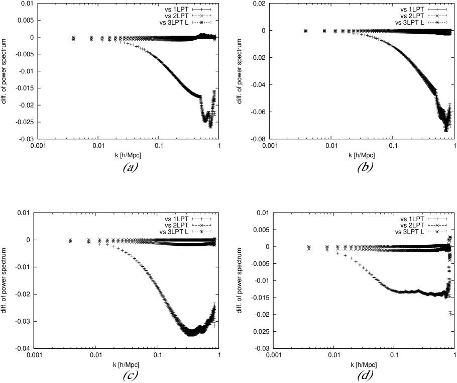
Figure 1: The difference between the power spectrum of the density distribution with the initial conditions based on 3LPT and other perturbations: (a) $z=10$, (b) $z=5$, (c) $z=2$, (d) $z=0$. The error bars are given by the difference between samples.

3.3 Non-Gaussianity

Next, we notice a a one-point probability distribution function of the density fluctuation field ${\mathcal{P}}(\delta)$ the probability of obtaining the value $\delta$ plays an important role. If $\delta$ is a random Gaussian field, the PDF of the density fluctuation is determined as

$${\mathcal{P}}(\delta)=\frac{1}{(2\pi\sigma^{2})^{1/2}}e^{-\delta^{2}/2\sigma^{2}}\,,$$ (22)

where $\sigma^{2}\equiv\left<\left(\delta-\left<\delta\right>\right)^{2}\right>$ is the dispersion and $\left<\;\;\right>$ denotes the spatial average.

In this paper, we set the initial condition by random Gaussian field. If the growth of the density fluctuation is linear, the density field still be Gaussian. The expected tools to detect transients at large scales are the cumulants of the one-point PDF of the density fluctuation field whose orders are higher than two which become nonzero for the distribution deviating from Gaussian. In the structure formation, non-Gaussianity are generated because of the non-linear dynamics of the fluctuations, even though $\delta$ is initially treated as a random Gaussian field, as a result of the generic prediction of inflationary scenario.

For this purpose, we concentrate on the third and fourth order cumulants, which are defined as $<\delta^{3}>_{c}\equiv<\delta^{3}>$, $<\delta^{4}>_{c}\equiv<\delta^{4}>-3\sigma^{4}$ display asymmetry and non-Gaussian degree of “peakiness”, respectively, for a given dispersion [1, 4]. Since it is known that the scaling $<\delta^{n}>_{c}\propto\sigma^{2n-2}$ holds for weakly non-linear regions during the gravitational clustering [7] from Gaussian initial conditions, we introduce the following normalized higher-order statistical quantities :

skewness $$: \gamma=\frac{\left<\delta^{3}\right>_{c}}{\sigma^{4}}\,,$$

kurtosis $$: \eta=\frac{\left<\delta^{4}\right>_{c}}{\sigma^{6}}\,.$$

The merit of adopting these definitions is, as stated above, that they are constants in weakly nonlinear stage which are given by Eulerian linear and second-order perturbation theory [1, 7]. For example, in the E-dS model smoothed with a spherical top-hat window function (Eq. (21)), the skewness and the kurtosis are given by

$$\gamma = \frac{34}{7}+y_{1}+{\cal{O}}(\sigma^{2})\,,$$ (23)

$$\eta = \frac{60712}{1323}+\frac{62}{3}y_{1}-\frac{7}{3}y_{1}^{3}+\frac{2}{3}y_{2}+{\cal{O}}(\sigma^{2})\,,$$ (24)

where

$$y_{p}\equiv\frac{d^{p}\ln\sigma^{2}(R)}{d\ln^{p}R},$$ (25)

with smoothing scale $R$ [7].

For this form of the skewness and the kurtosis, the effects of transients at large scales from the ZA initial condition is also investigated by [33, 34] as

$$\gamma_{\rm tran} = -\frac{6}{5a}+\frac{12}{35a^{7/2}}\,,$$ (26)

$$\eta_{\rm tran} = -\frac{816}{35a}-\frac{28y_{1}}{5a}+\frac{184}{75a^{2}}+\frac{1312}{245a^{7/2}}$$ (27)

$$+\frac{8y_{1}}{5a^{7/2}}-\frac{1504}{4725a^{9/2}}+\frac{192}{1225a^{7}}\,.$$

In the analysis of the non-Gaussianity, as we showed in Paper I, the dispersion among samples is quite large. In this subsection, we do not show error bars in figures.

Fig. 2 shows the difference of the evolution of the density dispersion and non-Gaussianity. Here we choose smoothing scale $R=1h^{-1}$ [Mpc]. The dispersion increases monotonically. The difference of the dispersion with the initial conditions based on 3LPT and ZA is less than $2\%$. In other words, the effect of higher-order perturbations seems percent order. Then the difference between dispersion with the initial conditions based on the 2LPT and 3LPT perturbations is less than $0.1\%$. For the dispersion, the effect of 3LPT seems almost neglectable.

The difference between non-Gaussianity with the initial conditions based on the ZA and higher-order perturbations seems percent order. Therefore, when we require $1\%$ accuracy for the non-Gaussianity, at least we should apply 2LPT for the initial conditions. Furthermore, when we require $0.1\%$ accuracy for the non-Gaussianity, at least we should apply 3LPT for the initial conditions. For non-Gaussianity, the effect of 3LPT transverse mode is quite small. Because the difference of non-Gaussianity with the initial conditions based on 3LPT varies between samples, it is hard to discuss the effect of the transverse mode in 3LPT for the initial condition.

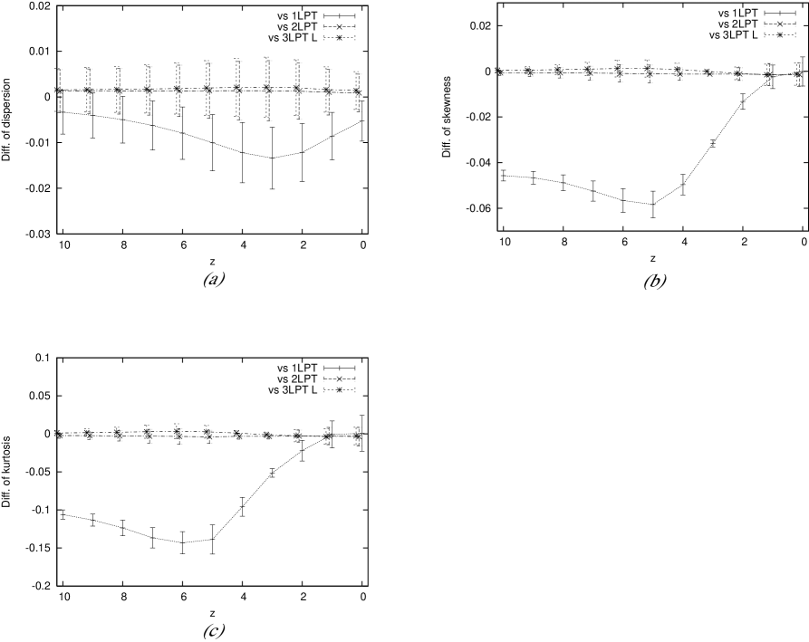
Figure 2: The difference of the dispersion and non-Gaussianity of the density distribution from N-body simulation ($R=1h^{-1}$ Mpc). Here we compare 3LPT and other perturbations. In order to make the difference legible, plots are slightly shifted. (a) The difference of the density dispersion. (b) The difference of the skewness. (c) The difference of the kurtosis.

4 Summary

Recently, observations constrained several cosmological constants. In order to compare theoretical predictions with observations, high accuracy for cosmological simulations has been required. In precise simulations, a setup of initial conditions becomes one of most important problem.

In this paper, we have discussed initial condition problem for cosmological $N$-body simulations with Lagrangian perturbation theory (LPT). In standard method, Zel’dovich approximation (ZA), i.e., first-order LPT (1LPT) have been applied for the initial conditions for a long time. However, it is well known that ZA is insufficient for description of the evolution for non-Gaussianity in the density field. The reason is the existence of so-called transients, that is, the most dominant decaying mode arising from our ignorance of the initial conditions. Crocce et al. [20] pointed out the effect of the transient for non-Gaussianity with initial conditions based on ZA and 2LPT. They show that although 2LPT decreases the effect of the transient compared with ZA, it still remains. In statistics quantities, such as non-Gaussianity and the spectrum, the difference of several percent appears among both. Then in Paper I [21], we analyzed the non-Gaussianity with the initial conditions based on 1LPT, 2LPT, and 3LPT. Since 3LPT initial conditions are expected to provide exact results for the kurtosis in the weakly non-linear region, we can evaluate the impact of transients from 2LPT initial conditions. The initial conditions are set up at $z\simeq 20,30,80$. When we set the initial conditions at $z\simeq 80$, the difference between the non-Gaussianity with the initial conditions based on 2LPT and 3LPT almost disappears. In Paper I, the transverse mode in 3LPT was ignored.

We have analyzed the effect of the transverse mode in 3LPT. In addition to non-Gaussianity, the power spectrum has been analyzed. In all the comparison, the difference of statistical quantities with the initial conditions based on 2LPT and 3LPT is sub-percent order. In other words, when we require more than $1$ % accuracy, we should set up initial conditions for cosmological $N$-body simulations with 3LPT. Then the effect of the transverse mode in 3LPT seems quite small. In the analysis for density field, the transverse mode in 3LPT would be ignored.

Why the impact of the transverse mode in 3LPT is quite small for the density field? We can explain the reason by the description of the density fluctuation with the Lagrangian perturbation. Here we expand Eq.(3).

$$\delta = -\nabla\cdot\bm{s}+\left(\nabla\cdot\bm{s}\right)^{2}-\frac{1}{2}\left(\left(\nabla\cdot\bm{s}\right)^{2}-s_{i,j}s_{i,j}\right)$$ (28)

$$-\left(\nabla\cdot\bm{s}\right)^{3}+\left(\nabla\cdot\bm{s}\right)\left(\left(\nabla\cdot\bm{s}\right)^{2}-s_{i,j}s_{i,j}\right)$$

$$-\det\left(s_{i,j}\right)+\cdots\,.$$

The leading order of Eq.(28) is given by the divergence of the Lagrangian displacement vector. The longitudinal mode of 3LPT causes third-order effect for the density fluctuation. On the other hand, by the definition, the divergence of the transverse mode of 3LPT disappears. Therefore the transverse mode of 3LPT gives fourth-order effect for the density fluctuation. Here we set up the initial conditions in high-$z$ region, the impact of the transverse mode would be quite small. When we have interested in peculiar velocity or the density field in redshift space, the transverse mode in 3LPT would affect as large as the longitudinal mode in 3LPT.

Finally, we briefly mention applications of our study to observations of the near future. Several projects which survey galaxies around $z=1$ are carrying out or planning [35, 36]. These results show not only the result of structure formation but also its evolution. By comparison of theoretical prediction and observation, it is expected that severe restriction is given to the nature of dark energy. Quite high-precision theoretical prediction is required for this comparison. Our study about the initial conditions will contribute to cosmological simulations for restricting dark energy models.

References

References

- [1] Peebles P J E 1980 The Large-Scale Structure of the Universe (Princeton: Princeton University Press)
- [2] Padmanabhan T 1993 Structure Formation in the Universe (Cambridge: Cambridge University Press)
- [3] Sahni V and Coles P 1995 Phys. Rep. 262 1
- [4] Peacock J 1999 Cosmological Physics (Cambridge: Cambridge University Press)
- [5] Liddle A R and Lyth D H 2000 Cosmological Inflation and Large-Scale Structure (Cambridge: Cambridge University Press)
- [6] Coles P and Lucchin F 2002 Cosmology, The Origin and Evolution of Cosmic Structure (Chichester: John Wiley)
- [7] Bernardeau F, Colombi S, Gaztanaga E, Scoccimarro R 202 Phys. Rep. 367 1
- [8] Jones B J, Martínez V J, Saar E, Trimble V 2004, Rev. Mod. Phys. 76 1211
- [9] Weinberg S 2008 Cosmology (Oxford: Oxford University Press)
- [10] Riess A G et al. 1998 Astron. J. 116 1009
- [11] Schmidt B P et al. 1998 Astrophys. J. 507 46
- [12] Perlmutter S et al. 1999 Astrophys. J. 517 565
- [13] Weinberg S 1989 Rev. Mod. Phys. 61 1
- [14] Peebles P J E and Ratra B 2003 Rev. Mod. Phys. 75 559
- [15] Copeland E J, Sami M, Tsujikawa S 2006 Int. J. Mod. Phys. D 15 1753
- [16] Hockney W R and Eastwood W 1981 Computer Simulation Using Particles New York: (McGraw-Hill); Bertschinger E and Gelb J M 1991 Computers in Physics 5 (2) 164
- [17] Tatekawa T 2005 Recent Res. Devel. Astrophys. 2 1 [arXiv:astro-ph/0412025].
- [18] Tatekawa T and Mizuno S 2010 in Dark Energy: Theories, Developments, and Implications (K. Lefebvre and R. Garcia, eds.) (New York: Nova Science), 241
- [19] Zel’dovich Ya B 1970 Astron. Astrophys. 5 84
- [20] Crocce M, Pueblas S and Scoccimarro R 2006 Mon. Not. R. Astron. Soc. 373 369
- [21] Tatekawa T and Mizuno S 2007 J. Cosmo. Astropart. Phys. 12, 014
- [22] Buchert T 1992 Mon. Not. R. Astron. Soc. 254 729
- [23] Barrow J D and Saich P 1993 Class. Quantum Grav. 10 79
- [24] Bouchet F R, Juszkiewicz R, Colombi S and Pellat R 1992 Astrophys. J. 394 L5
- [25] Buchert T and Ehlers J 1993 Mon. Not. R. Astron. Soc. 264 375
- [26] Buchert T 1994 Mon. Not. R. Astron. Soc. 267 811
- [27] Bouchet F R, Colombi S, Hivon E, and Juszkiewicz R, Astron. Astrophys. 296 575
- [28] Catelan P 1995 Mon. Not. R. Astron. Soc. 276 115
- [29] Sasaki M and Kasai M 1998 Prog. Theor. Phys. 99 585
- [30] Ma C P and Bertschinger E 1995 Astrophys. J. 455 7
- [31] Komatsu E et al. 2011 Astrophys. J. Supp. 192 18
- [32] Eisenstein D J et al. 2005 Astrophys. J. 633 560
- [33] Scoccimarro R 1998 Mon. Not. Roy. Astron. Soc. 299 1097 [arXiv:astro-ph/9711187].
- [34] Valageas P 2002 Astron. Astrophys. 385 761
- [35] Dawson K S et al. 2013 Astron. J. 145 10
- [36] Newman J A et al. 2013 Astrophys. J. Supp. 208 5